Numerical ODE solvers that preserve first integrals

Rochester Institute of Technology

RIT Scholar Works

Theses

Thesis/Dissertation Collections

2000

Numerical ODE solvers that preserve first integrals

Thuya Aung

Follow this and additional works at:

http://scholarworks.rit.edu/theses

This Thesis is brought to you for free and open access by the Thesis/Dissertation Collections at RIT Scholar Works. It has been accepted for inclusion

in Theses by an authorized administrator of RIT Scholar Works. For more information, please contact

[email protected]

.

Recommended Citation

NUMERICAL ODE SOLVERS

THAT PRESERVE FIRST INTEGRALS

By

Thuya Aung

A thesis submitted in partial fulfillment of the

requirements for the degree of

MASTER OF SCIENCE

m

Mechanical Engineering

Josef Torok (Thesis Advisor)

Professor

-Approved by:

Professor

-Hany Ghoneim

Professor

-Kevin Kochersberger

Professor

-Satish Kandlikar (Department Head)

Department of Mechanical Engineering

College of Engineering

ACKNOWLEDGMENTS

I

would

like

to

thank

my

thesis

advisor, Dr. Josef S.

Torok,

for his time,

guidance and

input

on

this thesis.

This

thesis

itself

would

benefit

for

my further

research studies.

Dr.

Torok

had

provided me with

support,

encouragement,

and resources

necessary

to

complete

this

thesis.

I

also would

like

to thank

him

for

being

such a

fun,

a

knowledgeable

and an

outstanding instructor

of

many

of

my

classes.

I

appreciate

him for

this

fun

and

learn

thesis.

I

also wishto thank

my

parents,

Mr.

Maung

Htay

and

Mrs. Khin

Thit,

and

my

relatives:

Mrs. Khin

Htwe,

Mrs. Kyi K. P.

Tun,

Ms. Khin

Chit,

Mrs. Nu N.

Yee,

Mr. Ye

Myint,

Ven. U

Okegansa,

Mr. Khine T.

Kyaw,

Mr. Wilson

Tun,

Ms. Hla M.

Swar,

and

Mr. Zarni

Y.

Yint,

for

being

so

supportive, understanding,

and

encouraging

as

I

completed

my

TABLE OF

CONTENTS

Chapter

Page

1

.

General

overview

1

2.

Background

4

2. 1

Introduction

to

Lagrangian Dynamics

4

2.2

Introduction

to

Hamiltonian Dynamics

13

3.

Analytical

Prediction

of

Conservative

Systems from

the

Hamiltonian

and

First Integrals

25

3.1

Energy Preserving

Algorithms

25

3.2

First Integral from Euler-Lagrange Equations

40

4.

Numerical ODE

Solvers

that

Preserve First Integrals

42

3.1

Orbital Derivatives

and

First Integrals

42

3.2

Integral-Preserving

Numerical Integrator Systems

48

5.

Summary

and

Conclusions

83

6.

References

86

CHAPTER

1

GENERAL

OVERVIEW

Quantity

measurement of

the

change

in energy

by

a

force

from

any dynamical

action

has been

used

for

modern

dynamical

mechanics.

Newtonian

mechanics need a

free

body

diagram

to

analyze

positions,

velocities, accelerations,

and

forces acting

on

any

dynamical

systems.

From

a

free

body diagram,

vectors are another

thing

thatwe

have

to

keep

track ofcross and

dot

products,

so

Newtonian

mechanics

is

required to

know

the

analysis of vectors or vectormechanics.

Momentum

and

forces

are essential

features in

vector mechanics.

Unlike Newtonian

mechanics,

analyzing energy

methods requires

knowledge

of

kinetic

energy

and potential

function.

Since

kinetic

energy,

potential

functions,

and work are scalar

quantities,

we

do

not

have

to analyze vector mechanics.

By

analyzing

energy

along

with variational

calculus,

Lagrangian

Dynamics

and

Hamiltonian Dynamics have been

established.

In

Chapter

2,

we review these two

dynamics

systems

in

terms of

how

they

were

developed

and

how

they

were used

in

mechanics.

Understanding

ofconstraint would also

help

in

modern

dynamical

mechanics.

In

Newtonian mechanics,

the constraint

forces

such as

boundary

conditions and

initial

conditions are required to

be

known

in

addition

to

applied

forces.

Because

coordinates

used are

dependent

onthe

system,

we need

to take

account of all

the

constraint

forces.

However,

using

generalized coordinates

that

are

independent

of

the

system

(we

will also

review

in

Chapter

2),

we can embed constraint equations

that

will

be

seen

in

Lagrange's

space

is different

than that

in

configuration space

(collection

ofgeneralized coordinates).

For

example,

a

freely

moving

particle

has

three

degrees

of

freedom in

space and six

degrees

of

freedom

for

generalized

coordinates,

three

for

position and

three

for

orientation,

in

configuration space.

Having

six equations of motion

in

configuration

space rather than

three

equations of motion and constraints

in

space,

for

Newtonian

mechanics,

this particular example

is embedding

the

constraint equation

into

the system

of equations.

Therefore,

it is

easier

to

solve

for

the constraints

because

constraints

in

configuration space are adjoined

to the

problem

formulation

as side conditions.

Thus

we need

to

discuss

briefly

the classification of constraints.

There

are

four

kinds

ofconstraints:

holonomic,

nonholonomic, rheonomic,

and scleronomic.

There

are

two

forms

ofequations

that

will consider

holonomic

constraints;

they

are either surface

constant ortime

dependent.

fix\,

x2,

X3)

=constant and

/(xi,

x2, X3,

t)

=

constant

Nonholonomic

constraints are constraints that cannot

be

expressed

in form

of

holonomic

constraints.

Some

examples of

the

rate of changes are

inequalities

and

nonintegrable

differential

expressions.

g(xx,

x2,

x3,

/)

>

0

A\dxx

+

A2dx2

+A-idxT,

+Aodt=

₀

Rheonomic

constraints are constraints

that

time, t,

appears

explicitly

at

least

in

a

constraint

for

agiven system of equations

(like

nonautonomous equations).

Scleronomic

constraints are constraints

that

time,

/,

does

not appear

explicitly in any

constraint

for

a

all

kinds

of constraints that are embedded

into

systems of equations and solve

for

them

numerically.

Once

we get

the

solution

from

Lagrange's Equations

of

Motion (Chapter

2),

the

result

describes

a single point

in

the

configuration space.

Because analyzing energy

methods are

based

on

kinetic energy

and potential

functions,

we should

have

scalar

quantities suchasthe resultwas a single point.

An

infinite

number of

different

solutions

may be

encounteredwith

different

velocities at the same point.

For

example,

a simple

spring-weight oscillator can

have different

velocities at a single position

(slower

and

faster

velocities will

be

encountered at

the

same point

in

the middle of a

spring

while

oscillating).

Therefore considering

position and

velocity

independently

will

be

much

more valuable.

The

motion ofa point

in

theplane

is

analyzed

by having

one axis

for

the

position and the other

for

the velocity.

This

is

called a phase

space,

and

it is

the

logical

plane

for

analysis.

In

later

Chapters

we will

discuss

numerical solutions of a system ofequations

by

Lagrangian,

Hamiltonian,

and

First Integral solutions,

like holonomic

constraint system

(explained

in later Chapters).

Lagrangian

systems are

holonomic

systems

for

whichthe

forces

are

derivable

from

a generalized potential

function

V(q,q,t),

and so are

Hamiltonian

systems.

Again,

since results are scalar

quantities,

wecantake advantageof

solving

them numerically.

When

compared with conventional numerical methods

that

are applied

to

the equations of motion of classical

mechanics,

such quantities conserve

the

total

energy

and momenta

only

in

the

order of

the truncation

error;

round-off errors

CHAPTER 2

BACKGROUND

2.1

INTRODUCTION LAGRANGIAN

DYNAMICS

To

systematize equations of

motion,

coordinates used should

be

independent

of

the system.

Thus,

generalized coordinates are

introduced.

Although

a

freely

moving

rigid

body,

as an

example,

has

three

degrees

of

freedom,

it

can

be determined

by

six

coordinates:

three

coordinates

is

for

the

position ofthe center ofmass of

the

body

and

three

others

for

the

orientation of

the

body

in

space.

Therefore,

a

freely

moving

rigid

body

that

is like

two

independent

masses

moving

freely

in

space,

requires a total of six

coordinate specifications.

The

details

of units arenot

important

as

long

asthe six values

uniquely describe

the configuration of

the

system.

The

collection of all possible points

withthecoordinates

is

called configuration space.

Before

we go

into Lagrangian

Dynamics,

we need

to

discuss

about the

kinetic

energy

of a system

because both Lagrange

and

Hamilton

analyzed

dynamics

based

on

energy.

A

singleparticle

moving in

space

has kinetic energy

as,

T^^mj^xf

(2.1.1)

1=1

In

here,

x

is

atotal

time

derivative.

If

we choose

qx, q2,

and _qj, are generalized

coordinates,

we must

have

transformation

between

the

physical and generalized

coordinates

as,

x, =

Taking

total

derivatives

to the transformation

withrespect

to time

will

be,

dx.

dqj

ai

dxi

~dt

(2.1.3)

Substituting

absolute

velocity

of

(2.1.3)

into

(2.1.1),

the

kinetic energy

of a

particle

becomes

(using

tensor

analysis),

T

=

\m

-m

dx,

.

dx

-Qi + [

dq]

J

dt

. \

dx,

.

dx,

dqk

dt

(2.1.4)

dxi dx,

. .

dx,

.

dx,

dx,

.

dx,

-q,qk +

q,

+

Qk

d<lj

Sqk

dq}

dt

dqk

'

dt

Kdt _j

2\

sothat

where

=

\m

dx,

dx

i i

dq;

dqk

. .

dx, dx,

. .

oqi

dt

dxt

3 3

T

=

1Z

Z

ajk4j4k

+

Z

PAi

+

y

j=X k=X ;=i

dx, dx.

dx, dx,

a, --

fi.

-m "'"' ""' and

y

--

\m

jk

dx,

~dt

dq;.

dqk

' '

dqj

dt

Thus,

the

kinetic energy

is

transformed as a scalar

function

ofthe generalized

coordinates and velocities.

T

=

T(q,q-,t)

(2.1.5)

Likewise,

for

an

N

particle system

in

three-dimensional

space,

absolute velocities

ofthe system are

x,

= '-=

>

dt

%

dx.

1j

dx

+

^-

(2.1.6)

dt

dqj

Also,

the total

kinetic

energy

ofiV-particle system

in

terms ofthegeneralized coordinates

and velocities

is,

3jV 3AT 3iV

;=1 k=X j=X

again,

T

=

T{qj,t)

(2.1.8)

which

has

total of

3./V

generalized coordinates and

3N

generahzed velocities.

Grouping

with respect

to the

powers of

the

generalized

velocities,

we can write

the total

kinetic

energy

as,

T=T2

+

T!

+

T0

(2.1.9)

Also

generalized

momentum,

pt, is defined

as the rate of change of the total

kinetic energy

with respectto a particular componentofgeneralized

velocity

qt

.

P,=~

(2.1.10)

dq,

Both Lagrangian Dynamics

and

Hamiltonian

Dynamics

are

based

on analysis of

energy along

with variational methods.

Therefore,

instead

of

generating

the equations of

motion

from free

body

diagrams,

we will analyze

the

variation of

energy

and the

minimum number of coordinates to characterize

the

dynamics

of

the

system.

The

formulation

of

the

dynamics

problems

in

terms

of generalized coordinates

is

called

The governing

equation

in

vector

form for

the

i-th

particle

is,

dp,

F

,

= _m

,a

dt

(2.1.11)

We

will now analyze

the

analytical mechanics.

The

time rate of change ofthe

generalized momentum

corresponding

to

the

-th-generalized

coordinate

is,

d

. .

d

Pk=~dt{Pk)

=

Jt

r dT^

(2.1.12)

Because

of

the total

kinetic

energy

of the system

for TV-particles

systems

in

Cartesian

coordinates

is,

T

=

^mi(xf+yf+zf)

(2.1.13)

Thus

pk

becomes,

Pk

=

dT

Zw,

dqk

dqk

dqk

(2.1.14)

Using

the

transformation

from

(2.1.6)

and

taking

partial

derivatives

with respect

to

q becomes

dx

,

dx

,

d4k

dak

Thus,

equation

(2. 1

.

14) becomes,

ffT

"

p. = = _{/ m}

Pk

dqk

{

'

Also,

taking

time

derivative

becomes,

.

dx

dy,

.

dzi

dqk

dqk

dqk

d_

dt

'

dT

"

^<ik

,

(2.1.15)

(2.1.16)

Pk

=

Z

mi

1=1

N

..

dxi

..

^v,

..

dz,

x: -+

yi

-^-+ z.

Z

w.

1=1

$<lk

'

dt

dqk

'

dqk

dxi

KdakJ

+

y,

d_

dt

_\d(ikj

+ z.

d_

dt

f

dz.^

dq

\~ik j

(2.1.18)

According

to

Newton's

Second

Law,

the

first

summationof

(2.1.18)

becomes,

m ,x;

F,

m,y,

F.

For

thesecond summationof

(2.

1

.

1

8),

we will again use equation

(2.1.6)

dx

and

replacing

x with

in

the

equation,

and

its derivative

withrespect oftimewill

be

dlk

d_

dt

r dx,^

dq

K^Vk J "

d

z~

71

dl,

dx.

dq

ij

+ y^'ik j

d_

dt

f

dx,^

dq

\^ik j

^

d2xt

.

d2x,

V

'

q

, +

-%

dq}dqk

dtdqk

d

dq,

J^

dx,

.

dx,

y

-q

, +

-%dq/J

dt

d_

dt

dxi

ydqk j

d

r. l

dx

lxi\

dq

&<li

where n

is

the

coordinates,

and

TV is

number ofparticles.

Thus,

equation

(2.1.1

8)

becomes,

Pk

=

d_

dt

rdT^

dq

Qk+Tmi

\^ik_J i=i

.

dx,

.

dy,

.

dy,

Qk

+

d

dqk

Qk

+

dT

Z *=₁

2 2

+

^,

+ z

>!)

3qk

Therefore,

the

Lagrange's Equation

of

Motion

becomes,

f dT^

dt

dT

\dqk)

dq

=

Qk

(2.1.19)

We

will now

briefly

discuss

three

different

types

of

Lagrangian Dynamic's

systems.

They

are

Conservative,

Non-conservative

and

Dissipative Lagrangian

systems.

Conservative Lagrangian Systems

For

a conservative

system,

L

=

T

-V

,where

Fis

a generalized potential

function

usually

given as

V =V{q)

(2.1.20)

Therefore,

Q,

dv

#qk

and

dV

dqk

as we

have

usually

seen.

Thus,

the

Lagrange's Equation

of

Motion

becomes,

d_

dt

d_

dt

d_

dt

d(T(q,lt)-V(q))

dqk

dT(q,lt)

dVjq)

-

Sdk

~

-<%

$qk

Therefore Lagrange's

equations of motions

are,

Pk

d(T

_-V) _

dL

dqk

dqk

d

d(T

-V) _

dT

dV_

dL_

dt

dqk

dqk

dqk

dq

k

(2.1.22a)

(2.1.22b)

Non-conservative Lagrangian Systems

For

a non-conservative

system,

assuming

generalizedpotential

function

V

exists

in

a

way

that

is

given

as,

Q

~-^

dt

dV(q,q,0

dqk

dV(q,q,t)

dqk

(2.1.23)

If

we substitutethegiven generalized

force

into Lagrange's

equations

(2. 1

.

19),

we

have

d_

dt

dT(q,q,t)

dqk

dT(q,

q,t)

_

d

dqk

dt

dV(q,q,t)

dqk

dV(q,q,t)

Sqk

(2.1.24)

Since

L(q,

q,

t)

=

T(q,

q,

t)

-V(q,

q,

t)

,weget

d_

dt

dL(q,q,t)

dqk

dL{q,q,t)

dqk

(2.1.25)

We

cannot

say

the above equation

is

conservative system although

(2.1.25)

is

similar to

(2.1.21)

because

the generalized potential

function does

not

depend

on

the

generalized coordinates only.

Therefore

a conservative system

is

a special case of a

Lagrangian

system.

For

the

general non-conservative

system,

not

assuming

the

generalized potential

function

as

(2.1.23)

or not

derivable from

a generalized potential

function,

we can split

Qk

=Qlom ₊

Q,

knone

dv

dqk

+

Qk

(2.1.26)

wherethe conservative component

is

derivable from

apotential

function.

Thus,

constructing

the

Lagrangian

function L

=

T

-V,

we

formulate

the

Lagrange's

equations of motion

as,

d_

dt

SL(q,q,t)

Sqk

dL(q,q,t)

$qk

=

Qn;

fc=\,2,...,n

(2.1.27)

where

Q"kc

are generalized

forces

which

is

not

derivable from

apotential

function.

Dissipative Lagrangian

Systems

If

we

have dissipative

systems as

FIX=~CXA

F

--c v

iy yiSi

F

=-c z.

IZ Z, I

The

virtualwork

done

by

these

dissipative forces

undera set ofvirtual

displacement

is,

5W

=

YJF-br=

-Z(^i,^:, -r-c^fy,

+czi,&J

(2.1.28)

1=1

where

"

dx

5x,.

=

V

-5^

and

8r

=

0

Also,

using

equation

(2.1.15),

dx

,

dx

dq

k

dqk

thevirtualwork

done (2.

1.28)

becomes

5W

=

-Yj

k=X

V

d

(

dq.

xf+cjf+cziz2)

k=\

^Hk

%tk

Therefore

in

general we can split more on

Qk

as,

dV

where

Qk=Qcr

+Qnr

+d=-^-+q:+d

^k

D

=

\jlcxx2+cyiy2+c2tz2)

k=X

(2.1.29)

(2.1.30)

(2.1.31)

D

is

known

as

Rayleigh's Dissipation Function.

The Lagrange's

equations of motion

then

is,

d_

dt

dL(q,q,t)

&Lk

dL(q,q,t)

_|

dD(q,q,t)

dqk

dqk

(2.1.32)

where

Q*k

is

a generalized

force

which

is

not

derivable from

a potential

function

or a

2.2

INTRODUCTION

HAMILTONIAN

DYNAMICS

Now

we show

how

to

transform

Lagrangian

Dynamics

into

Hamiltonian

Dynamics.

We

can review

the

Legendre

Transformation

for

the connection

between

Lagrangian

and

Hamiltonian functions.

If/(x)

a

twice-differentiable

function

which

is strictly

convex,

/"(x)>0

(2.2.1)

and

let/? be

a

tangential

coordinate

defined

as

P

=

/'(*)

The Lagendre Transformation is

given as

g(p)

=

xp-f(x)

so that

dg

dx

df

dx

dp

dp

dx

dp

and

(2.2.2)

(2.2.3)

PX~

g(j>)

=

px-(xp

-/(x))

=

f{x)

Therefore,

Lagendre Transformation

has

a

property

that

p

is

the tangential

coordinate

for

g(p)

andx

is

the

tangential coordinate

for/(x).

Therefore

is

completely

symmetrical.

, -r- _{/ x i i}

dq>(x)

,. .

1

.

loge

,

As

an

example,

if

(p{x)

=

log

x

, then

p

= =(loge)- _so

that

_x =

and

dx

x

p

<p(x)

=

log

p

J

Thus

finally,

the

Legendre

transformation

of

(p{x) is

g(p)

=

px-<p(x)

=

log

_e

-log

=

log

Cx

\

loge

r

_e

^

V

P

J

Now

we can

apply

a

Legendre

transformation to

a

function

of several variables.

Let/(xi,

x2,

...

,

xn;

y\,y2,...

ym)

be

a

function

ofn+m variables where

det

d2f

dy,dy

,.

*

0

(2.2.4)

We

introduce

new coordinates

/'=

1,2,

...,m 5 *~J '

>

(2.2.5)

Now

we can

define

the

Legendre

transformation

of/

with respect

to the

variables

ji,^2,...^mas

g(xh

x2,...,xn;zi>z2,...,zm)=

Z^,2!

-/ 1=1

dg

dx

.

IL

dx

.

where k=

1, 2,...,

w.

(2.2.6)

(2.2.7)

Also,

/(xi,

x2,

...

,

xn;

zh zx

..._,

zm)

=

Z

>^,- " g"

(2.2.8)

Again

the transformations are

completely

symmetrical

like in

one-dimensional

case.

There

is

one more

property

that

is

the variables

xi, x2,...,

_xn

do

not

actively

participate

in

the

transformation.

Therefore,

the

dual

function

H,

the

Hamiltonian

function

transform

from

Lagrangian function

through

Legendre Transformation

then

is

H

=

Xp,<ii-L

1=1

Lagrangian function

can

then

be

rewritten with

the

Hamiltonian

as

=

Zm,-#

(221)

i=i

where

dq

,

dq

.

Thus,

if

we want to write so-called

Hamilton's Canonical

Equations,

similar to

Lagrange's

equations,

we

have

p. =

(2.2.12a)

P'

dq,

but for

the

q

_i notice

the

generalized coordinates

qt

are not transformed

by

(2.2.7),

therefore

dH

,

qt

=

2.2.12b

dpt

Thus

we

have

atotalof

2n

first-order differential

equations.

An

example of

Hamilton's Canonical Equation

of

Motion

is

given

below.

H

= _{+ -PjLT+}

f".

2

-+

V(r,0J)

2m

2mr2 2mr2 sin2

9

v ' ,rj

The

canonical equationsare:

=

cH=P^

cpr

m

'

a

dH

pe

dpg

mr

1

m

0

= :

P

*

mr2sin2

6

dH

Pi

Pi

dV

dr

Pr

'

dr

mr3 mr3sin2

6

dH

p}cos0

3V

For

the

Hamiltonian,

one more

property

can

be

observed.

Since both Hamiltonian

and

Lagrangian both

were established

from

kinetic energy expressing in

terms of

generalized momenta and generalized

velocities,

wewill

look

very

closely

on

distinguish

the

two

expression.

Hamiltonian is

also a

form

of

energy

with expression

in

terms

ofthe

generalized momenta

instead

of generalized velocities

because

generalized coordinates

are not

transformed

for

the

generalized

velocities;

we can compare

(2.1.22)

and

(2.2.12).

Therefore,

T\

from

the

(2.1.9)

is

zero.

Therefore

h

=

YpA

-l=

(t2

+T0)h

-(T2+T0 -V)l

1=1

H=T2-T0+V

by

(2.2.

11)

Furthermore,

for

natural

systems,

the

kinetic

energy

is

purely

quadratic

in

the

velocities.

That

is

T=T2

and sothe

Hamiltonian

is

and

To

=

₀

H=T+V

which

is

the total mechanical

energy

ofthesystem.

The

timerateofchange of

the

Hamiltonian

is

(2.2.13)

dH

dt

dH

dH

.

qt

+ _~z

P.

dq,

dp,

+

dH

dt

The

summation represents the

implicit

dependence

on

t through the

coordinates

and momenta.

The

last

term represents

the

explicit

dependence

of

the

Hamiltonian

on

time /.

If

we substitutethecanonical

equations,

dH

.

dH

q,

dp,

and

Pt

=

we

have

dH

"

x . . . . -,

dH

-aT=Zx[-p-q- +

q'p^-dT

dH

dH

,

-Ji-^r

(Z214)

The

total mechanical

energy

is

conserved

that

is

a special case

for

the

Hamiltonian

(such

as

the

conservative systems are the special case

for

the

Lagrengian

Dynamics).

Conservative in here

means

the

autonomous

system, time

is

not

explicitly

express

in

the

system ofequations

that

is

shown

in (2.2.14).

Therefore

the

interesting

statement

is

that

the

Hamiltonian

function H

is

a constant

throughout the

evolution ofthe

system.

That

is,

the

Hamiltonian

is

an

integral

of

the

motion

(also

called

first

integral

of

equation,

we will

discuss

on

later

sections), representing

the

conservation of some portion

oftotalenergy.

Furthermore,

since

t

is

not active

in

the

Legendre

transformation, it follows

from

the

property

(2.2.7)

that

dH

dL

,

^r--^r

(2215)

which means

that

thevariable t appears

in

the

Hamiltonian

if

and

only if

t

appears

in

the

Lagrangian

function.

If

we consider

the

Hamiltonian

as

the

velocity

field

of

fluid

in

the

Eulerian

description

such

that the

vector

fields

are given as

*i

=FM,Xi,()

The

collection ofcurvesthatare

tangent to the

velocity

field

at

any fixed instant

oftime are calledsteamlineswhich can shown as =

Fx

F2

If

fluid is

incompressible,

there

is

no change

in

volume ofparticles moves

along

the

flow

field;

theshape

may

change

during

themotion.

Thus

the

incompressibility

ofthe

fluid is

,. ,_

dFx

dF2

_

div(y)

=

L+

- =

₀

dxx

dx2

Therefore,

the

Hamiltonian

in

a stream

function

for

the

flow

ofan

imaginary

fluid

in 2-dimensional

space

becomes

^v(v)

=

Z^L+Z^L=0

(2-216)

,=i

dq,

~

dp,

where

Fx

= q,=

and

F2

=

p,

=

--dp,

dq,

sothat

tt

dp,dqf

i=x

dq,dp,

Therefore using Liouville's

Theorem,

we can

build

Hamiltonian (Example 2.2.2).

There

is

one

thing

to

be

notedthat

div

(v)

=

0

does

_not

necessarily

means

the

conservativesystemof

Hamiltonian;

it just

means

Hamiltonian

can

be

easily

built

(Example 2.2.2).

In Chapter

3,

We

will

discuss how

tocheck

analytically

whether

if

the

given

Hamiltonian

is

conservativeornot.

Some

examplesof

transforming

from Lagrangian

to

Hamiltonian

orvise

visa,

verifying Hamiltonian

systems

using Liouville's

Theorem,

and

finding

the

Hamiltonian

Example 2.2.1

If

the

Lagrangian

is

givenas

using (2.

1.22a)

L

= _-*-x 2

-\a>

2x2

+ exx 2

-5x

dL

dL

. .

/> = = _x = =

2

_{x +}

2

_xx

<?# <?x

and

(2.2.9)

H-^PA

-L=pq-L=

(2x

₊

2xx)x-\x2 +xx2

i=i

H=\x2 +\co2x2 +xx2

+3c3

Thus

the

Hamiltonian

can

be determined.

Analyzing

example

2. 2.

1,

if

weassume we

have T

=\x2 ₊

exx2

and

V

-\co2x2

+dx3 ,

conservativesystemwith

T2

and

T\

=

To

=

0,

thenwe can

clearly

define

Lagrangian

system,

L

= T-

Fand Hamiltonian H

=

T+V. See

example

2.2.6.

Example 2.2.2

In

orderto

determine if

system of equations

is

Hamiltonian,

we use

Liouville's Theorem

onthat system of equations ofaparticle

in

two

dimension.

ydq,

|

y

dp,

=

dx,

_|

dx2_=l

1

=

Q

Therefore Equations

in

example

2.2.2 satisfy Liouville's Theorem

and

it

is

a

Hamiltonian

system.

Thus,

we can construct a

Hamiltonian

equation

using

potential

function

approach.

xx=^Sr^=xx+x2

OX}

H(xl,x2)=xxx2A+F(xx)

and

^^=x2+F(xl)

2

caq

Also,

Sf/fex,)

-x2=^r2l=-xx+x2

oq

Therefore,

F'(xl)

=

-xx and

F(xx)=-^+C

Finally,

#(x1,x2)

=_x1x2+|--'|+C

We

will usethis example

in later

sections.

Example

2.2.3

x1=xx+2x2

*2~X, ~X2

Again using Liouville's Theorem

to

determine

if

thesystemofequations are

Hamiltonian,

tt

dq,

t=i

dp,

dxx

dx2

We

can also use

Liouville's Theorem

for

nonautonomous systems

to

find

Hamiltonian

such as

Example

2.2.4.

Example

2.2.4

X,

=xxt-2x2

Again using

Liouville's

Theorem

to

determine

if

the

system of equationsare

Hamiltonian,

f^

+

f^P=dxL+dx^=t

+

(2^0

1=1

dqi

,=,

dp,

dxx

dx2

Therefore

thegiven system

is

nota

Hamiltonian

system

Example 2.2.5

Xj

=xit+2x2

Again using Liouville's Theorem

to

determine if

the

system of equations are

Hamiltonian,

fdq^+ydpi_=dx^+dx^=t_t

=

0

tt

dq,

,=x

dp,

ax,

dx2

Therefore

the

given system

is

a

Hamiltonian

system

H(xx,x2)=xxx2t+x;+F(xl)

and

*^=^+F(j<)

Also,

Therefore,

9>q

F'(x1)=-x1r2

and

F(xx)=-^-+C

Finally,

if

(x

Xj)

=

x,x/

+x^

- _+C

Example

2. 2.

6

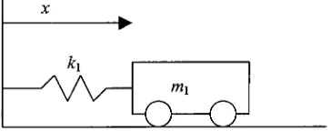
Consider

a mass

that

only

a

spring

attaches

to the

wall. [image:26.529.154.336.312.384.2]

mx

Figure 2.2.1 A

mass

is

attached

to

thewall

only

by

a

spring

Kinetic

andpotential

energy

ofthe system will

be

T-\mx2

V^+^mx2

and

because

the system

is

conservative, the

Lagrangian

will

be

L

=T-

V

=

\

mx2

l-mx2

or

for

our

convenience,

L

=

so

that

dL

.

dL

p- =

mq

and p= =

-mq

dq

"

dq

H

=pq-L=

mq2

~mq2)=

\mq2+\mq2

Therefore,

H=\mx2+\mx2=T+V

We

can also prove

that

Hamiltonian

is kinetic

energy

plus potential

energy for

conservative systems.

Example 2. 2.

7

If

oneofthecanonical equations

for

asingle

degree

of

freedom Hamiltonian

system

is

givenas

p=p2-2q+2p

then,

we can

find

H because

dH

2 n

p=-=p2-2q+2p

dq

H(qp)=-p2q+q2-2pq+F(p)

and

q

=

^-

=

-2pq-2q+F'(p)

(2.2.17)

dp

Also,

we can

determine^

because

it's

a

Hamiltonian

system,

so

Liouville's Theorem

has

to

satisfy

such

that

dq

q

=

-2pq-2q +

F(p)

(2.2.18)

Comparing (2.2.17)

and

(2.2.18),

we

find

that

F'(p)=F(p)

sothat

F(p)

can

be

either exponential or zero.

If

zero

is

simple,

wecanchoose

F(p)

to

be

ep.

Therefore,

q

=

-2pq

-2q

+ep

and

H(q,p)=-p2q+q2-2pq+ep

also

if

we want

to

convert

H

to

L,

weneed

qp

=

-2p2q-2pq

+pep

Thus,

I{qp)

=qp-H=-2p2q-2pq+-pi

+p2q-q2

+2pq-ep

CHAPTER

3

ANALYTICAL PREDICATION

OF

CONSERVATIVE SYSTEMS

FROM THE HAMILTONIAN AND FIRST INTEGRALS

3.1

ENERGY PRESERVING ALGORITHMS

For

theapplication of

the

Hamiltonian,

we need

to

introduce

the

energy

preserving

algorithms.

The energy

preservation shows some

interesting

propertiesof

conservation

in Hamiltonian. It is

given as

Man+x+K(dn+x)

=

Fn

(3.1.1)

dn+x=dn+^At{vn+vn+l)

(3.1.2)

v+i=v+!-Aa(a+0

(3.1.3)

(3.1.4)

(3.1.5)

(3.1.6)

where

U

is

thepotentialthatgenerates

K

,

i.e.,

DU

=

K

.

This

algorithm obeys

the

identity

E(dn+l,vn+1)

=

E(dn,vn)

₊

^(dn+l

-dJ(Fn+l

+Fn)

(3.1.7)

The

energy-preserving

algorithm

(3.1. l)-(3. 1

_.6) can

be

defined

for

ageneral

Hamiltonian

system

(finite

or

infinite-dimensional)

as

well,

dp

dq

2

-

2[U(dn+x)-U(d)]

A

-'<?-

x~dn)W

J+K(dn)\

d0

=

d

In

which:

qn+l=q

^Si^J^kMA

(3.1.9)

AT(P+X-Pn)

i"

(qn+i-qn)

^

=

^r{ccqn+x+(l-a)qn,/Jpn+x

₊

(l-P)pn)

(3.1.11)

and;

^

=

(w+i +

(i-r)^,^+i

+

a-^)A)

(3.1.12)

where

a,

/?,

/,

^are

arbitrarily

chosen

in

the

interval

[0,1].

For

theproof of conservation of

energy,

Equation

(3.

1.9)

becomes,

A

Take

transpose

to

both

side

then,

((^+i-l)-(P+i-A))

A/

Also

(3.1.10)

becomes

=

H(qn+1,pn+x)-H(qn+x,pn)

(3.1.13)

<H(qn+x,pn)-H(qn,pn))

At

=

subtracting

(3.1.14)

from

(3.1.13)

becomes

(fart

-g,)fori -Pn)J -{(Pr^X ~A)@^1 -qn)J _n_pre

- v W--x

---"(4H.iAfi)--n(4,,/'J

so

that

H(fLvPn+x)=H(qn,pn)

Example 3. 1. 1

Example

in

simple

harmonic

Oscillator

since n=

1,

one

particle,

.

#/

.

a?/

,

<i=-r=p

and

p=-r-=-a>q

dp

dq

andwe want toshow

the

system

is

conservative

using energy preserving

algorithms.

So,

dH

*

=

~r-(aq+1 +

(1

-a)qn,/3pn+x

+

(1

-/?)/>)

dp

^

=

/K+i+0

-/?)/> and

^r=l

and

then,

dH

p

=

^-(rqn+x +

0

-r)qn,^Pn+x

+

₀

-<?)/>

)

y"=

2(w+i

+

0-r)?J

and // = /;

qn+x

=

qn

+

At

f

^2^,2 _2

'>\

<

qn+x

,

ft+1

A

^,22 -2

A

l+Al

Pn+X~Pn

qn+x

=qn

+

2

Pn+X~Pn

At.

.

qn+i

=

qn+(pn+x+Pn)

(3.1.15)

ft+1

=p-to

(H(qn+x,Pn)-H(qn,pn))

(qn+x-qn)

Pn+X

=Pn~At

f

2 2 2

A

f 2 2 2"N

g gg

ft

2

2

4*+l

-?

ft+1

=

ft

2

?+1

-?

ft+i=ft"

2-A/

(qn+x+qn)

(3.1.16)

Now

we

have

two

finite difference

equations such

(3.1.15)

and

(3.1.16)

2 2 2

If

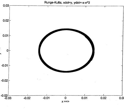
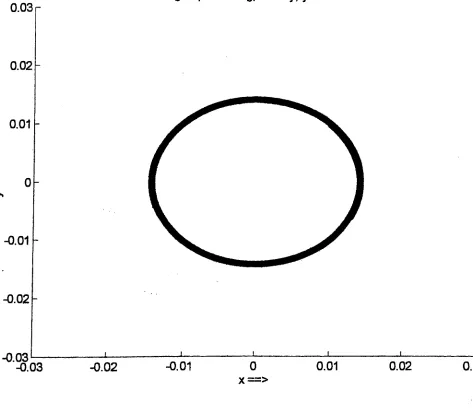
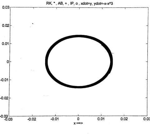
we can proofH(qna,pnhl)=H(qn,pn)= +=constant, the system will

be

conservative,

andthephase curve will

be

elliptical.

Thus,

^i,fti)=^+f

:

qn+^(PrX+Pn)

21

2

J

V

^

_at-ti

CO-tor

s

&+^-(fti+ft)

+-2

ft

fe

-i-^fom

+ft)+^}

'

2

(A)2

^

+^(fti +ft)+^(ft,

+ft?

/

A,

^-fl?-A-A{22I-^(ftfl+jRl)}

4

^(A)2^

A

{2^^-(fti+ft)?

where (A)2 0

Thus,

6J2 2

o^to.qn

ql+

-2

2

ft2 (Pml+Pn)+~Or-^-P^n-

col(toyPn

(ft+1

+Pn)

again (A)2

0,

Therefore,

co2

2

dtStqn

co2Atq

p2

, a

=

y^

+^p^

Jr~rp-2

'p"q-o? 2

,

^a^,

^qn,p2n

4^^^-ft)+4

andwe

know

from

(3.1.16)

that

ft+i

"ft <y2-A/

(<7,i+i

+,)

Therefore

H(q^pn+x><Tn+-Y~ at-tt

(*+,)

^

Pi

o} ,

<a\tof<L(

since(A)2

0,

3. 2

^q^P^ql

+y

=H(qn,pn)=

constant.

Therefore

we proved

that the

given simple

Harmonic Oscillator Hamiltonian

system

is

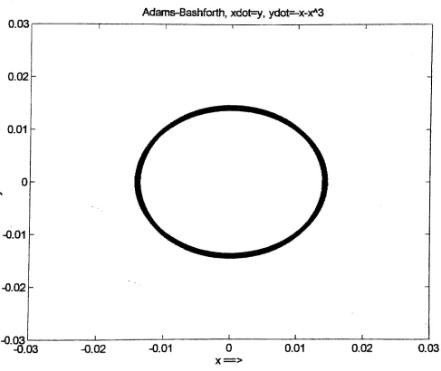
conservative.

We

will now

find

out whether

the

given

Duffing

equation

is

conservative or not

using energy preserving

algorithms.

Example 3.1.2

We

know

the

given

Duffing

equation

does

not

have

damping

so

that

x+x3+x=0

So

wecan write

x=y

y=-x-x3

By

using Liouville's

Theorem,

Y^l

₊

v

^

=

^+^Uo

₊

o

=

o

tt dq,

tt dp,

dx

dy

The

system

is

Hamiltonian.

Thus,

dH

dH

y2

x=

q

= =

=p

=

y

and

H(x,y)=^-+F(x)

dp

dy

2

M

F'(x)

also

ax

, .

dH

dH

y

-X + -X ~

-p =

Thus,

F'(x)

= _x+

x:

x2 x4

and F(x)- 1

2

4

Finally,

TT.

y2 x2 x4

H(x,y)=+ +

2

2

4

or

for

our convenience

set,

where,

H(q,p)Ml+l

2

2

4

.

dH

.

dH

,

v=t:=p

and _-p=^-=q+q

dp

dq

We

nowshow

that the

system

is

conservative

using

energy preserving

algorithms.

So,

*

=

~{ctqn+x+(\-a)qnJpn+x+(\-(3)pn)

dp

^

=

/?ft+i+0-/?)ft

and X7 =X

and

air

/" =

(j?,+)

+

0

-r)q,#pn+x

+

₀

-)ft)

/"=rfe+i+?l,)+0-r)(^+^) and /" =/*

then.

qn+x

=_qn+At

(H(qn+l,Pn+x)-H(qn+x,pn))

(ft+i

-ft)

(2 4 2

^

^n+1

.

^+l

,

ft+1

v

2

'

4

'

2

;

-^2 4 2

>

#n+l

,

^n+l

.

ft

In+X

qn

+

^HpIx-pI)

2

ft+,

_-ft

qn+X=qn+(Pn+X+Pn)

(3.1.17)

In

here,

do

not

try

to

solve ln+X _ l

At

V

qn

+

(ft+i

+

ft

)

and set (At)2

0

.

qn+x

and

pn

2

J

areto

be

solved simultaneously.

Pn+x=Pn-At-

(H(qn+X,pn)-H(qn,pn))

(qn+i-qn)

Pn+X

=Pn~At

(

2 4 2"\

^n+i

.

q+\

.

fti

,242,

-/ 2 4 2>

q*

+qn +

pn

V2

'

4

'

2y

ft+1

=

ft

A4fe+i)-fc)l

A/[fe+i)-fa)j

2

^+i-<?

4

?+1-tf

ft+i

=P*~Y

(q"+l

+q")~~^

(^"+1

+

q"

)(^+1

+

^"

}

(3 l 1

8)

Now

we

have

two

finite

difference

equationssuch

(3.1.17)

and

(3.1.18).

Using

these two

equations

for

thenext point

in

H,

H(q^Pn+x)=^

<L

+,

<L

,

Pr

L

2

4

2

substituting (3

.

1

.

1

7)

and

(3

.

1

.

1

8)

into

(3.1.19)

(3.1.19)

f

to

Y

J

f

q+^iPn+X+Pn)

+i

(

\

2

;

V

&+r(ftl+#l)

A

A

A

A

T

A

Y

2

ft

(,+^-(fti

+ft)+^)--fe+^(fti +ft)+^)k

+^(fti

+ft)J

+)

setting

(A/)2

ite

+toq,(Pn+x +p))+i(q2 +Atq,(p^x

+pn)f

+-,

Pn

~(H)~Q4ni{

+toqn(Pn+l

+Pn)}+C)

lk

+toq,(p^

+Pn))+ik

+TH<P*A +ft))

At I2

ft

~toq --qn(2ql

+tiq,(pn+x

+pjj

-4

=|fe

+^4(fti

+ft))+ife

+2A^fe+1 +A))-4(r.

"*4

-^f

=

I

fe

+**(?,,

+ft))+i

(qi

+2&&P,*

+ft))+l

(ft2

-2AM

-2A^)

=I^+-^>^i+ft)+i44+Y^(fti+ft)+ift2-Aft^-A^?^

Now,

we substitute equation

(3.1.18),

soweget

,,

A

4^+~4

ft

"-(4+i

+4)--(4+i

+4)(42+,

+42)+ft

1

w*

ft

~

(4+i

+4)

--(4+i

+4)(42+i +4") +ft

+i4

HPl-topAn-Atpd

again,

setting

(A/)2

0

=i42+y4[2^J+i44+Y43[2ft]+lft2-A^^-A7J^

Wn+topqn+H+topdHpl-top^-^pd

Therefore,

2 4 2^242

L/Y^ \

^"-1

i

^l

i

ft+!

4

.

4

.

ft

rr/ x ,

^+i>ft+i)=+ +=y+

+Y=^(4>ft)=co5to/?/

Therefore

we proof

the

givensystemof

Duffing

equations

is

conservative.

The

Runge-Kutta,

xdot=y,

ydct=-x-xA3

0.03

r

0.02

0.01

-0.01

-0.02

-0.03

[image:38.529.20.502.178.613.2]

Example 3. 1.

3

From

example

2. 2.

2

H(xx,x2)

=_xxx2+^-5-+C

For

our

convince,

let C

=

0,

H(qp)=qp+^--^-To

show

the

above

Hamiltonian

is

conservative or

not,

we can again use

energy

preservation

algorithms,

So,

it

follows

that:

and,

Then,

m

q==q+p

and

dp

dH

.

dH

-p==-q+p

dq

A

= (aqn+l+(l-a)qn,fi>n+l+(l-j3)pn)

dp

*

=

4+i

+

₀

-a)qn

+

/K+i

+

(1

-P)pn

with XT =

X

dq

m

= -m+1 -

(i

-r)4

+

SPn,x

+

₀

-^)ft

with pr

-p

4+i=4+A>

(H(qn+X,pn+X)-H(qn+X,pn))

(ft+i

-ft) 4+i=4+^

f

2 2 >

t/+l Fn+X

-'

V

I I j

-(

2 2^

4'ft-^f

+

v

V

l l j

4+i

=

4

+

AKftVft2)

2

ft+i

_-ft

At

r

4+i

=4+y(ft+i+ft)

(3.1.20)

In

here,

do

not

try

to

solve tn+X _ i

A*

V

4

+

(ft+i

+

ft

)

and set (Ar)2 *

₀

.

qn+x

and

p+1

1

J

are

to

be

solved simultaneously.

Hence

. AAH(qn+x,Pn)-H(qn,pn))

(4+1-4)

ft+1

=Pn~At

Vf

2 _2> A 2 2Al

4+i

ft

4

+

ft

4,+,

ft,-4,

ft-v

2

2

J

v

2

2

J

'n+l

ft

+

4+i

-4

Mfc+J-fe)]

A,(4+i~4)ft

2

4i+i

-4i

!-A^-fn+l

4

Aft

N A

ft+i

=ft+y(4+i+4)-A*ft

ft+i

=ft+y((4+i+4)-2ft)

(3.1.21)

Now

we

have

two

finite

difference

equations such

(3.1.20)

and

(3.1.21).

Using

these

two equations

for

the

next point

in H.

H(qn+x,pn+x)=q,x-pK+x+^-Y

(3.1.22)

substituting (3.

1.20)

and

(3.

1.21)

into

(3.

1.22)

(

to

V

A/

4+-(fti+ft)

ft+-((4+i+4)-2ft)

2

)\

2

(

a

y

r

a

ft+-((4+i+4)-2ft)

4

4+-(fti+ft)

2

;

v

2

4

1

Y

setting

(At)2

0

=4

P

+-4((4+i

+4)~2ft)+-ft(fti

+ft)

+lfc +Atpn{(qnX

+qn)-2pn))-l(ql +Atq,(pn+X

+pjj

We

again substitute

(3.3.20),

A

=4

'ft

+4

A

4

+^(fti +ft)+4

-2ft

l+-ft(fti

+ft)

A

+:

/

A

A

+top!

4

+-(#*, +ft)+4

-2ft

I

-\(ql

+toqn(PnA

+pjj

V 2

A

(

=4

-ft

+4

+:

A^

^ ^

1

to

,

H

+~^(Pmi

+Pn)-2Pn\+Pn(Pn+X +ft)

A

/

+%[

24

+-(fti +ft)-2ft

j

Ufe

+toq(pMX

+Pjj

setting

(Ar)2

0

A

=4

'ft +A-42

-AtqnPn

+-pn(pn+x

+p)

+\(pl +2JstqnPn

-2Atf)-\(

+lq,(pM

+pjj

A

=4

'ft

+^

-A-4P

+-ft(ft+i

+ft)

We

now substitute

(3.

1.21),

so we get

=4

-ft

+A4 +p

pn

+-((4+i +4)-2ft)+ft

2 _V 2

ft

41

A/.

A,

+f

"

A^

-|

-dfl

+-((4+!

+4)

-2ft)

+ft

=4

'ft+

A^

+-/J

2p

+-((qnhX +qn)~2pn)

Pn

to.

At,

+f

"

A^

-|

4l

2ft

+-((4+i +4)

-%J

again,

setting

(Ar)2

0

2 2

--qn-Pn+toql+topl+^-titi-^-Atm

2 2

:4-ft+^f+A/4(4"ft)

Therefore

22 22

#(4+i,ft+i)

=4+i

"ft+i

+^y

-Y

=4

-ft

+y

-|

+A^fe

-a)

*#(4,ft)

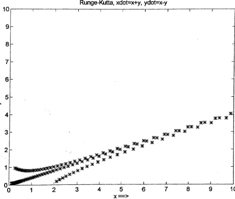
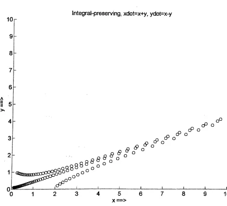
^constant

Therefore

we proof

the

given systemofequations

is

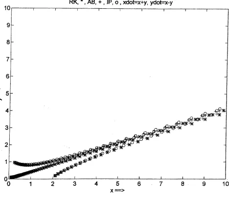
not conservative.

The

phase

curve will not

have

closed contours.

In

this example,

we showed

that

conservative

systems are a special case of

Lagrangian

or

Hamiltonian

systems.

Not

all

Hamiltonian

10

Runge-Kutta,

xdot=x+y,

ydot=x-y

-i 1 r -i 1 r

8

7

6-A II II O

3fc

as*. ^ *

5l6if *

ae* *

2K* * 5K* *

ftjtf****

J I 1 I 1 L

3456789

10

[image:43.529.33.498.188.583.2]

x=>

3.2

FIRST INTEGRAL FROM EULER-LAGRANGE EQUATION

From

Euler-Lagrange

equation,

we

have

dy

dx

dy'

where

F is

a

functional,

a

function

ofa

function,

such as

F=F(x,y,y')

andwe

have

second orderequation

dy

fdF^

dx

dy

dx

+

-fdF^

\"s J

dy

\dy j

dy

+

dy'

^dF^

dy

dy'

Vvy

There

are

two

special cases

from Euler-Lagrange

equations.

Case I

If

F is

a

functional

of

function

xand

y

'

,

F

=

F(x,y')

then

the

Euler-Lagrange

equation

becomes

'(x,

dy

dF(x,y')

= _constant

because

dF(x,y')

dy

=

0

Case II

If ftis

a

functional

of

function

v and

y'

,

F

=

F(y,y')

then

the Euler-Lagrange

equation

becomes

(3.2.1)

F(y,y')-y,<9F(X'y>}

=_constant

(3.2.3)

dy'

Equation

(3.2.2)

and

(3.2.3)

are

first-order differential

equations.

One less

equation

has

to

be integrated.

Physically,

a

first

integral

represents

the

conservation ofa

certain quantity.

The

left-hand

sides of equation

(3.2.2)

and

(3.2.3)

represent the

CHAPTER

4

NUMERICAL ODE SOLVERS THAT PRESERVE FIRST INTEGRAL

4.1

ORBITAL

DERIVATIVES

AND FIRST INTEGRAL

As

we

have discussed

on page

2

of

Chapter

1,

equations

in

whichthe

independent

variable

/

does

not occur

explicitly

are called autonomous equations.

A

vector equation

ofautonomous can

be

written as

x =

f(x)

(4.1.1)

In

here,

we call equation

(4.1.1)

an autonomous

differential

equation

because

t

does

not

explicitly

appear

in

the

equation.

A

point

in

phase space with coordinates _xi

(t),

_x2

(t),

...

, xn

(t)

for

certain

t, is

called a phase point.

In general, for

increasing

t,

a phase point shall move

through

phase-space.

In carrying

out

the

projection

into

phase

space,

we

do

not

generally know

the solution curves of equation

(4.1.1),

but it is

simple to

formulate

a

differential

equation

describing

the

behavior

of

the

orbits

in

phase space.

Equation

(4.1.1)

can

be

writtenout

in

components as

x,

=

/,(x)

;/'=

1,

...,

We

now use one of

the

components of

x,

such as

xi,

as a new

independent

variable.

In

order

to

getx\

to

be

such

independent

variable,

fx

(

x

)

*

0

.

Therefore

^=/,W

and

%=/*(*)

dt

dt

and

dividing

dxx

into

dxk

, we

have

dxk

=

dfk(x)

dxx

fx

(x)

k

=

2,...,n

Example 4. 1. 1

Harmonic

oscillator x + x =

₀

The

equivalentvectorequation

in

with x =

xx

, x =

x2

The

orbitsofgiven

two

dimensional Phase

space are

described

by

dxx

x2

Integration

yields

x2

+

x2

=_constant

Or using Liouville's

Theorem,

fdq^

+

fdP=^+^=0_0

=

₀

ttdq,

ttdp,

dx,

dx2

Therefore

the system

is

a

Hamiltonian

system

_dH(xx,x2)_

m,*d=^+m

and

^^=F(xi)

2

oq

Also,

Therefore,

_dH(xl,x2)_

-Xi--\

a^

x2

//(x1,x2)=|+|+C

H(x,x)-C=^-+~

2

2

Solutions

of system

(4.1.2)

in

phase space are called orbits.

In

equation

(4.1.2),

time

has been

eliminated,

so

it

can

be integrated

in

a number of

cases,

producing

a

relation

between

the

components of the solution vector.

Since

simple

harmonic

oscillator

is conservative,

H(xh

x2)

=

C

is constant,

differentiation

withrespect

to

t

gives,

xx+xx=

x(x+x)

=

₀

Now

we will

introduce

the

concept of orbital

derivative.

Let

ft

be

the

orbital

derivative.

Consider

the

differentiable

function

T

R"

^

R

and

the

vector

function

x:

R-*

R".

The

derivative

L,

of

the

function

/ along

the

vector

function

x,

parameterized

by

/,

is

T T

dl

.

dl

.

dl

.

dl

LJ = _x = _{x, + x. +}

... +

dx

dx,

<3x,

dx

"

l L n

If

we considertheequation x =

f(x)

, x e

D

a

R";

and

if

ft/

=

0,

then

I(x)

is

called

first integral

of equation.

In

example

4. 1. 1

_ __

dH

.

dH

, x

LtH

=

Xj

+

x2

=

XjXj

+

x2x2

= _xx+

x(-x)

=

₀

dxx

dx2

Therefore,

H in

example

4. 1. 1

will

be

a

first integral

ofequation

/.

If

a surface

is

constant or

if

the

rateofchanges are

integrable,

it

means

the

systemofequations

involve

Example 4. 1. 2

Let

us consider so-called

Volterra-Lotka

equations

x= _ax

-bxy

y

=

bxy

-cy

The

equation

for

theorbits

in

the

phaseplane

is

dy

_

x a_-by

dx

y

bx

c

Thus

the equation

is

separable and

integration

yield

bx

-cln x+

by

-a

In

y

=

C

=

I(x,y)

We

willnowcheckwith orbital

derivative,

, .

dl

.

dl

.

Lti

= _xh

y

=

dx

dy

\-<-"

(ax

-bxy)

+

f

b- a V

y)

(bxy

-cy)

V

xj

=

(bx

-c)(a

-by)

+

(by

-a)(bx

-c)

=

0

Therefore

resultant

7

(x,

y)is a

first integral

of

the

equation.

This may

also

involve holonomic

constraints.

However,

Volterra-Lotka has

some

interesting

properties

that

if

we now

let/?

=

In

x_{> x}=ep

and

q

=

In

v-

y

=_{e?the equations can}

be

_observed

as

Hamiltonian

x = ^- ₌

epp

=

(a-beq)ep

-p

=

(a-beq)

dp

dt

V r V '

y

=

^^-

=

eqq

=

(bep

-^q =

(bep

-c)

y

dq

dt

V r V '

H(q,p)

= bep

-cp

+ beq

-aq

dH

and

q

=

dH

dq

'

dp

Another

approach of

finding

a

first

integral

is

rather simple

for

conservative

problems.

Consider

example

3.1.2

and rewrite

two

system of equations

into

x+ x+

x3

=0

Where

we

introduce/^)

= _x+

x3

So

that

multiplying

by

x

becomes

xx+x(x+

x3)

=

₀

_{or \2x2)+}

\(x

_+x3)dx=

₀

dt

dt

-fex2)+-dtX2 '

dt

(2 4\ X X +

2

4

Therefore

the

first

integral

of

the

equation

is

then

1 C-2

x2 x4

I

=_{~x h} 1- =_constant

That

is just

the

advantage of

finding

the

first integral

equation

in

conservative systems.

Example 4. 1. 3

Let

usnow

look

atthree-dimensional systemofequations

Ax

=

(B

_-C)yz

By

=

(C-A)zx

Cz

=

(A-B)xy

The

equations

for

the

orbits

in

thephase plane are

dx_y(B-CV

B

^

dy

x

A

.

C-A_

((C

-A)A)x2

+

(B(C

-B))y2 =

Ix

(x,

y)

'c-aY

c

^

->

((C

-A)A)xdx

=

(B(B

-C))ydy

dz

y

B

J

A-B

->

((A

-B)B)ydy

=

(C(C

-A))zdz

((B

-A)B)y2

+

(C(C

-A))z2 =

Now

we

have

to

construct

in

a

three-dimensional

differentiable function /

=

I(x,

y,

z),

so we

have

to

use

the

so called

Lyapunov

function

construction..

If

we

let

y

=

z=

0,

thenx

becomes

arbitrary

such as x0.

Then, I\

or

L(x,

y)-I\(x0,

0)

is

not sign

definite in

a

neighborhood of

(x0, 0,

0)

and

I2

is

semidefinite.

One

of

the

ways to construct a

Lyapunov

function is

I(x,y,z)

=

[lJx,y)-IJx0,0)]2+I2(y,z)

=

[AC-A)^

+B(C-B)y2

-A(C-A)x$

-^B^B-A)/ +C(C-A)z2 2."4 2

7(x,

y,

z)

-2A2(C-A)2^x\

+B2(C-B)2y

+A2(C-Afx4

+5(5-^/

+C(C-A)z

We

willnow checkwithorbital

derivative,

T T

dl

.

dl

.

dl

.

LtI

= _xh

y

H z

dx

dy

dz

(4.1.3)

x=

[4^2(C-y4)2x3

+ 4A(C-A)B(C-B)xy2

-4A2(C-A)2xx20\^-^-dx

\

A

y=

\AA(C-A)B(C-B)^

v-4^(C-5)V -4ARC-A)(C-B)^y+2B(B-A)y\

^^

dy

\

B

yz

zx

z=

2C(C-A)z

dz

((A T>\\

xy

(A-B)

V

C

j

LJ.

=4A(B-Q(C-A)2x3yz+4B(C-A)(C-B)(B-C)xy3z-4A(C-A)2(B-C)xx2xyz

+4A(C-B)(C-A)2x3yz-4B(C-A)(C-B)2xy3z -4A(C-A)2(C-B)xxlyz

+

2(C-A)(B-A)xyz+ 2(C-A)(A-B)xyz

=

₀

Indeed,

the

resultant

/ in

(4.1.3)

is

a

first

integral

of

the

equation and give

4.2

INTEGRAL-PRESERVING

NUMERICAL

INTEGRATOR

SYSTEMS

In

the

last

section we showed

that the

first

Integral

of the

equation,

I(x)

is

a

constant

(4.2.1),

and

it is

typically

a

holonomic

constraint.

A

system of equations

that

involves

damping

can

be

thought

of as

embedding

of scleronomic

constraints,

because

time t

is

implicitly

involved. Consider:

I(x)

=_constant

(4.2.

1)

Taking

the time

derivative

gives

dl

dl dx

cl

dxn

d

dxn

= i-4-

-+ +

-=

0

dt

dxx

dt

dx2

dt

dxn

dt

_ =(v7). =

(V/)-F(x)

=

0

:-I(x)

=_constant

(4.2.2)

dt

dt

If

we

know

I

(xn)=

constant,

we should

be

able

to

construct

I(xn+X )

similar to the

energy preserving

algorithms

in Chapter 3.

Therefore,

as a

first step

we need to

find

a

skew symmetric

matrix,

S,

that

has

property

(ST

=

-S),

i.e.,

-S=

S2X

0

Now

we canconvert

the

system

to

skew-gradient

form:

[S(x)]\vi(x)]=^

=

F(x)

(4.2.3)

Multiplying

with

(V7)r

to

both

sideswillgive

(V/)r

[s\VI)

= (V/)r

F(x)

=

(VI) F(x)

(4.2.4)

Taking

the

transposeof

both

sides

((V/)r

[S](VI))T =

(VI)T[S]T

(VI)

=

(VI) F(x)

where

((VI)TJ

=

(VI)

is

obvious.

Also because

ST

=

(VI)T[S](VI)

=

(VI).F(X)

or

(VI)T[s](VI)

=

-iVI)-F(x)

Thus comparing

(4.2.4)

and

(4.2.5),

we

have

(4.2.5)

VI-F(x)=-VI-F(x)

or

V/F(x)

=

0

(4.2.6)

Equation

(4.2.6)

is

the

same as equation

(4.2.2).

Therefore

the

skew symmetric

matrix

does

not change

the

meaning

of

the

first

integral

of

the

equation that

is

/

is

constant.

Therefore,

we want

to

find

such

S,

skew-_{symmetricas a}

first

_step.

The

next

step

is

splitting.

The

n-

dimensional

_vector

fields

F

=

YFk

k=x

dxk

is

split,

using

the

skew-symmetry

of

S,

into