Rochester Institute of Technology
RIT Scholar Works
Theses Thesis/Dissertation Collections
2005
Evaluation of errors in national energy forecasts
Denys Sakva
Follow this and additional works at:http://scholarworks.rit.edu/theses
This Thesis is brought to you for free and open access by the Thesis/Dissertation Collections at RIT Scholar Works. It has been accepted for inclusion in Theses by an authorized administrator of RIT Scholar Works. For more information, please [email protected].
Recommended Citation
EVALUATION OF ERRORS IN NATIONAL ENERGY
FORECASTS
by
DENYS SAKVA
A thesis submitted to the Public Policy Program
of Rochester Institute of Technology
Rochester, New York
2005
APPROVED BY:
James Winebrake,
Ph.D.,
Chair
Public Policy Program, College of Liberal Arts
Ron Hira
, Ph.D., Assistant Professor
Public Policy Program, College of Liberal Arts
Mark Coleman
, Senior Program Manager
Table of contents
Abstract... 3
1. Introduction... 4
2. Literature review ... 6
3. Methodology ... 11
3.1. Overview... 11
3.2. Data ... 17
4. Total energy consumption decomposition ... 23
5. Transportation sector analysis... 34
6. Industrial sector analysis... 50
7. Commercial sector analysis ... 57
8. Residential sector analysis ... 65
9. Conclusions... 72
Abstract
Energy forecasts are widely used by the U.S. government, politicians, think tanks,
and utility companies. While short-term forecasts were reasonably accurate, medium and
long-range forecasts have almost always been highly erroneous. In the U.S. many energy
policy decisions are driven by Annual Energy Outlook (AEO) forecasts prepared by
Energy Information Association (EIA). This thesis evaluates accuracy of AEO reports
from 1982 to 2003. Parameters evaluated are: total energy consumption, energy
consumption by sector, sector specific parameters, and major model assumptions. Error
decomposition and regression analysis are used to appraise accuracy of forecasts. I found
that often underlying parameters used to calculate more aggregate parameters suffer from
errors that are higher by amplitude than forecasted parameter itself. Positive and negative
errors cancel each other and conceal higher error in the underlying parameters. Total
energy consumption was predicted with higher accuracy than energy consumption by
sector. Energy prices were predicted with very low accuracy and errors reach 250%.
Almost all parameters suffer from systemic errors and were consistently overestimated or
underestimated. I also determined numerical estimates for expected increase in accuracy
1.
Introduction
Rapid progress in computing power has transformed energy modeling and
forecasting into a popular and important business tool. The results of energy modeling
and forecasting are widely used by the U.S. government to develop a national energy
policy, by politicians and think tanks to advocate for or against various political
decisions, by utility companies to make investment decisions, and by many others. As
energy models become more complex and sophisticated, they may give a false sense of
accuracy and precision. Modelers and those who use the results of modeling are often
separate groups of people with different areas of expertise. Forecasts’ users often have
limited understanding of modeling principles and limitations; on the other hand modelers
may not understand what decision makers need (Munson, 2004). All of these factors may
lead to wrong decisions and overall disappointment in forecasting; as well as attract
attention to non-existent problems while ignoring most important issues.
Energy forecasts have a long history. While short-term forecasts were reasonably
accurate, medium- and long-range forecasts have almost always been wrong (Smil,
2003). Studying the accuracy of past projections will help to understand limitations and
ranges of applicability more fully, and to improve future predictions by avoiding past
mistakes.
In the U.S., many energy policy decisions and discussions are driven by
information and insights derived from energy forecasts. If measured by use in the
profession, the “gold standard” for such forecasts are those from the U.S. Department of
Energy’s (DOE) Energy Information Administration (EIA). The EIA has been making
National Energy Modeling System (NEMS) for over two decades through its Annual
Energy Outlook reports (1982-2004). The importance of these forecasts in defining the
energy debate cannot be understated.
Previous studies (Smil, 2003, O'Neill & Desaib, 2005) of the accuracy of energy
forecasts for the U.S. have indicated limited success in our ability to predict what the
energy landscape would look like 5,10 or 20 years hence. But these evaluations have
tended to analyze aggregate energy production and consumption. With this thesis, I
examine forecast errors within each major U.S. energy sector (transportation, buildings,
commercial, residential). I identify which sectors experience the greatest forecast errors
and whether these errors imply consistent over- or under-estimation of forecasts. I
explore each sector individually to find what parameters are most/least accurate and how
they contribute to sector error. I also examine the contribution of sectors to total energy
error. Finally, I explore whether these forecasts are improving over time. The results
presented in this thesis might help forecasters to improve their forecasts by determining
which sectors are most important in terms of influence on total error, and pointing out
2.
Literature review
Because of the importance of the accuracy of energy projections, many
researchers paid attention to how earlier energy forecasts predicted the future – our
present. Several attempts to analyze the accuracy of medium- and long-term energy
forecasts have been made. Some authors (Smil, 2003) argue the usefulness of energy
forecasts while others (Craig, Gadgil, & Koomey, 2002) think that energy forecasts are
still usable and useful.
William Ascher was one of the pioneers of comprehensive analysis of forecasting
errors. In his book, “Forecasting: An appraisal for policymakers and planners” (Ascher,
1978) he studied the accuracy of numerous population, economic, energy, transportation
and technological forecasts. Ascher sees accuracy as a best method for forecast appraisal.
He looked for similarities between forecasts and general trends in forecasting and drew
four major conclusions. First, time horizon is the most important factor that determines
accuracy. The longer the forecasting horizon is the less accurate forecasts are. Second,
forecasts produced during the same period of time appear to suffer from similar biases.
For example high oil prices forecasts published between 1997 and 2001 were under the
influence of relatively stable oil prices of 1990s (Smil, 2003). Third is that the choice of
methodology is having little influence on forecasting accuracy, and is much less a factor
than the choice of core assumptions. And finally the least accurate forecasts were often
based on outdated information or the forecaster missed some major changes in trends.
Ascher did not find any signs of improvement in forecasting of energy demand over time
(Ascher, 1978, p.125), he also found that no methodology offers substantially more
Vaclav Smil is one of the most active critics of current trends in energy
forecasting. In his book Energy At Crossroads: Global Perspectives And Uncertainties
Smil (2003) analyzed numerous forecasts of total energy consumption, prices and energy
intensities, energy consumption structure, and electricity demand and concluded
“long-range forecasters of energy affairs have missed every important shift of the past two
generations” (p.176) and “with rare exceptions, medium- and long- range forecasts
become largely worthless in a matter of years” (p.124). His analysis shows that almost all
U.S. and world energy consumption long-range forecasts for the year 2000 were greatly
overestimated. Apart from one forecast, all other analyzed forecasts were overestimating
world primary energy consumption by 10% to 200% and US primary energy
consumption by 20% to more than 200% (Smil, 2003). Even those projections that were
close had very different fuel consumption structures, and, thus, if used to forecast
emissions, fuel consumption by type, etc. would substantially offset derived forecasts.
World oil prices are another example of forecasters’ failure. Wild random fluctuations of
world oil prices over the last 30 years have made almost all forecasts rather useless.
Smil (2003) concludes that no model, no matter how complex it is, is able to
reflect and predict system behavior when extensive social, economic, technical, and
environmental interactions and change exist. Such interactions lead to unexpected events
that change the environment dramatically and are impossible to predict with any
reasonable certainty. He is against the use of complex computer models and quantitative
forecasting because they both need multiple numerical estimates and assumptions that, in
case they are inaccurate, propagate errors throughout the model. Smil(2003) proposes
forecaster is “outlining what should happen rather than what is likely to happen” (Smil,
2003, p179).
A different approach to analyze the accuracy of energy forecasts was used by
Craig, Gadgil, & Koomey (2002). They did not argue about the usefulness of energy
forecasts. Quite the contrary, they advocate forecasting as an instrument with many
purposes, such as “bookkeeping devices” that show a lack of good data; aids in selling
political ideas, which may be viewed as a form of normative scenarios proposed by Smil;
as training, educational and communicational aids that help to better understand a system
and communicate ideas between stakeholders; as aids to hypothesizing and what-if
analysis. Craig et al. (2002) analyzed several forecasting techniques by strengths and
weaknesses. EIA uses econometric models for its forecasts. The authors (2002) point out
that econometric models give reasonable projections when there are no structural changes
in a modeled system and perform best when used for short-term forecasting. Often they
produce results that are not better than much simpler models. (I want to point out here
that simpler models may not give enough information to solve problems that they were
designed to solve, such as effects of alternative energy policies.) Craig et al. (2002)
summarize their findings by the following recommendations to improve forecasts:
document assumptions as completely and as clearly as possible; define the range of
decisions this model will help to make; use a model that is simple enough for your tasks,
pay more attention to assumptions than to sophistication; do not underestimate changes in
human behavior in response to a changing environment; develop different scenarios; use
a combined approach by averaging several forecasts; assess risks and uncertainties; and
example of how forecasts should be created and communicated. They have extensive and
very detailed assumptions, they are explained and discussed at the annual conference,
they have several scenarios, and all information is publicly available since 1982 in
libraries or from the EIA web page.
Attempts to analyze AEO projections have been made before. The EIA has been
using a similar forecasting methodology and model structure for the last 20 years, which
greatly simplifies analysis of the model accuracy and accuracy progress over time. EIA
does such analyses by itself as in Sanchez (2002), Holte (2001). These are called the
Annual Energy Outlook Evaluations. The most recent evaluation available when this
thesis was written is for year 2002. In this paper EIA analyzes errors of most important
variables by calculating “average absolute forecast error … of all absolute values of
percent errors, expressed as the percentage difference between the Reference Case
projection and actual historic value, shown for each AEO, for each year in the forecast”
(Sanchez, 2002, para. 8). This type of analysis is appropriate to find years with highest
errors that may be a sign of something unexpected that happened in that particular year,
like oil price shocks. To analyze how forecasts’ accuracy is changing over time other
methods, such as decomposition (O’Neill & Desaib 2005) may be more appropriate.
O’Neill & Desaib (2005) applied a decomposition technique to analyze errors in
GDP, energy intensity and energy consumption for all AEO available. Their analysis
consists of calculations of the percentage error, absolute percentage error, mean
percentage error and mean average percentage error for the baseline error, trend error and
variability error. Analysis was made for total consumption and energy intensity without
energy consumption errors were low, while GDP and energy intensity errors were much
higher and had opposite signs, which introduced cancellation of errors. They find no
evidence of improvements from earlier projections to recent ones along with the increase
in the errors for longer projections. O’Neill & Desaib suggest paying more attention to
predicting GDP and energy intensity.
Linderoth (2000) studies forecast errors in International Energy Agency countries
by calculating forecast errors, average forecast errors and root mean square of forecast
errors for total primary energy consumption, oil consumption, delivered energy (total
energy minus losses) by sector and by country. He concludes that forecast errors are
caused by inaccurate growth rate expectations. In addition, energy consumption in the
transportation sector is generally underestimated. Similar to O'Neill & Desaib (2005) he
3.
Methodology
3.1. Overview
The thesis compare actual values with forecasted values to calculate percentage
error and then use an error decomposition technique to study errors of medium-range
forecasts for U.S. total energy consumption and consumption by sector. Decomposition
helps to identify the least/most accurate parts of the model, systemic
underestimation/overestimation of model components, and how forecasts’ accuracy
changes over time (are forecasts become more precise over time).
Armstrong (2001) gives the following definition of decomposition: “The process
of breaking a problem into subproblems, solving them, and then combining the solutions
to get an overall solution.” This thesis breaks total energy consumption error into errors
by sector. Then sectoral errors are broken into sector specific errors.
Most energy forecast error analyses in the past have focused on errors in projected
total energy production or consumption. One of the questions that remains unanswered in
such analyses is: How do each of the major energy sectors contribute to this overall
error? Oftentimes what looks like small errors in total energy forecasts actually hides
more significant (but offsetting) errors in specific energy sectors.
An error decomposition technique was applied to study errors in energy forecasts
by various energy sectors (commercial, industrial, transportation, residential) for the US.
In the US, total energy consumption projections (through NEMS) are determined through
an additive function across energy sectors. Thus, forecast errors within each sector will
contribute to the overall total forecast error. By breaking down total forecast errors into
more/less accurate and whether a systemic underestimation/overestimation exists within
sectoral model components.
I also explore how forecast accuracy changes over time across each of the major
energy sectors. That is, I address the question: “have US energy forecasters become
better or worse with respect to accurately capturing energy production and consumption
in the mid-term?”
I apply a methodology similar to that found in O'Neill & Desaib (2005). However,
unlike O'Neill & Desaib (2005), I focus on the “visible error” defined as “the difference
between the projected energy consumption and actual energy consumption” O'Neill &
Desaib (2005).
In this work I use two metrics to determine forecast error: mean percentage error
and mean absolute percentage error. Mean percentage error (MPE) is an average error of
all forecasts of a given forecast horizon and is given by the function,
τ τ τ τ τ n ) ( , , ,
∑
−= t t
MPE calculations for a single forecast horizon (τ) and a single year (t) (i.e., where
nτ = 1) could take on a positive or negative value. If MPE > 0, then the forecast value was
higher than the actual value, and the forecast represents an overestimate. If MPE < 0, then
the forecast value was less than the actual value, and the forecast is an underestimate. The
reader should note that an average MPE near zero does not imply a near perfect forecast.
The average may be close to zero, but may represent a combination of highly
overestimated and underestimated forecasts that cancel each other out on average.
To more clearly explore the accuracy of forecasts, without concern over whether
forecasts are underestimated or overestimated, I can apply the mean absolute percentage
error (MAPE), given by the following function:
τ τ
τ τ
τ n
) ˆ
(
, , ,
∑
−= t t
t t
Y Y Y
MAPE (2)
where the variables and indices remain the same as in (1). Here, however, the absolute
value of the error for each forecast is used, so that the metric is not subject to
misinterpretation from cancellation of under- and over-estimated forecasts. I apply both
the MPE and the MAPE on a sector-by-sector basis below.
Both MPE and MAPE identify sector-by-sector forecast errors, but they do not
allow for easy consideration of the contribution of these sectoral errors to total error.
Because the US delivered energy can be derived as an additive function of energy
consumption in all sectors, there is a clear connection between the forecast errors for each
sector and the forecast error for energy consumption overall. To determine the
Let the total forecast percent error (TFPEt,τ) for a given time horizon τ made at time
period t be:
(
)
∑
∑
∑
∑
∑
− = − = j j t j j t j t j j t j j t j j t t Y Y Y Y Y Y TFPE , , , , , , , , , , , , , ˆ ˆ τ τ τ τ τ ττ (3)
where j represents the set of sectors (commercial, industrial, residential, transportation).
Given equation (3) it is possible to determine that the contribution of TFPE from a given
sector (which is called the sectoral forecast percentage error for sector j, or SFPEj) is
given by:
∑
− =
j t j
j t j t j t Y Y Y SFPE , , , , , , , , ˆ τ τ τ τ (4)
The SFPEj can also be derived into a mean sectoral percentage forecast error (MSFPEj,τ)
for a given time horizon τ by modifying (4) as follows:
τ τ τ τ τ n ˆ , , , , , , ,
∑ ∑
⎟⎟ ⎟ ⎠ ⎞ ⎜ ⎜ ⎜ ⎝ ⎛ − = t j j t j t j t j Y Y YMSFPE (5)
After decomposing errors by components I used regression analysis to study
relationships between errors in model assumptions and errors in energy consumption,
energy prices, etc.
“Regression analysis is a statistical methodology that utilizes the relation between
two or more quantitative variables so that one variable can be predicted from the other or
A simple linear regression model can be presented in a following way (6):
x
y=α +β (6),
where α is the intercept of regression curve with y axis and β is a slope of the
regression line. To estimate parameters α and β the method of least squares was used.
To measure the strength of relationship a coefficient of determination r2 (7) was
used.
squares of
sum Total
regression of
squares of
Sum
2 =
r (7)
Coefficient of determination shows how much of total variability was explained
by using regression model. The closer the value of r2 to 1 the tighter the relationship is.
I expected that world oil price errors have most influence on transportation sector
energy price errors, and GDP errors have most influence on industrial sector consumption
errors. Oil is a major fuel and world oil price greatly influences average energy price and
prices of the other types of fuel. Real GDP was chosen because it is a good overall
indicator of economy development. Higher GDP levels mean that more products and
services are sold. Most of them require energy for production. I analyzed these
hypotheses using regression analysis methods. With the help of regression analysis I was
also able to find how strong the relationship between errors in assumptions and errors in
predicted variables are and how forecasts can be improved by using more accurate
assumptions.
Numerous factors may negatively influence accuracy of any forecast. Among
them are: incorrect core assumptions, unexpected random events that change behavior of
predicted parameters, inadequate methodology or internal model structure. Random
p.176). And as Ascher (1978) points out that choice of methodology is playing secondary
role in determining forecasts’ accuracy after the choice of core assumptions.
EIA uses extremely complex models to forecast all major parameters of energy
markets in the U.S. and the whole world. These models use numerous assumptions and
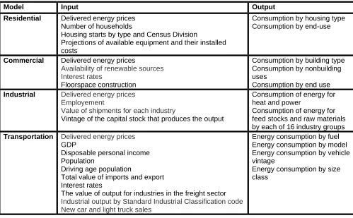
feedback loops. Table 1 shows selected assumptions for residential, commercial,
industrial and transportation sector models.
Using wrong core assumptions will negatively influence accuracy of the whole
model and negate all positive effects of correct methodology. Some model assumptions
(GDP) behave in a very predictable way, still they often suffer from systemic errors. I
will try to use simple models to forecast main assumptions and variables to check if it is
[image:17.612.90.589.409.718.2]possible to achieve better accuracy.
Table 1 - EIA models assumptions
Model Input Output
Residential Delivered energy prices Number of households
Housing starts by type and Census Division
Projections of available equipment and their installed costs
Consumption by housing type Consumption by end-use
Commercial Delivered energy prices
Availability of renewable sources Interest rates
Floorspace construction
Consumption by building type Consumption by nonbuilding uses
Consumption by end use Industrial Delivered energy prices
Employement
Value of shipments for each industry
Vintage of the capital stock that produces the output
Consumption of energy for heat and power
Consumption of energy for feed stocks and raw materials by each of 16 industry groups Transportation Delivered energy prices
GDP
Disposable personal income Population
Driving age population
Total value of imports and export Interest rates
The value of output for industries in the freight sector
Industrial output by Standard Industrial Classification code New car and light truck sales
Energy consumption by fuel Energy consumption by model Energy consumption by vehicle vintage
The military budge
3.2. NEMS description
The NEMS is a computer-based, energy-economy modeling system of U.S. energy markets for the midterm period through 2025. NEMS projects the production, imports, conversion, consumption, and prices of energy, subject to assumptions on macroeconomic and financial factors, world energy markets, resource availability and costs, behavioral and technological choice criteria, cost and performance characteristics of energy technologies, and demographics. NEMS was designed and implemented by the Energy EIA of the DOE (The National Energy Modeling System: An Overview, 2003).
The NEMS model breaks U.S. energy market up on smaller parts depending on energy usage. These smaller parts are modeled separately by NEMS modules. Additionally to U.S. energy market modules the NEMS model also includes Macroeconomic Activity, International Energy and Integrating modules. Currently EIA uses the following modules:
- Integrating Module
- Macroeconomic Activity Module - International Energy Module - Supply Modules
o Oil and Gas Supply Module
o Natural Gas Transmission and Distribution Module
o Coal Market Module
o Renewable Fuels Module
- Conversion Modules
o Electricity Market Module
o Petroleum Market Module
- Demand Modules
o Commercial Demand Module
o Industrial Demand Module
o Transportation Demand Module
Each module includes extensive regional information divided geographically. These regions include:
- Nine Census divisions for residential, commercial, and transportation consumption
- Four Census regions, shared to nine Census divisions for industrial consumption - Fifteen electricity supply regions (including Alaska and Hawaii) based on the
North American Electric Reliability Council regions and subregions for electricity supply and nine Census divisions for electricity demand
- Fifteen electricity supply regions for renewables
- Six lower 48 onshore regions, three lower 48 offshore regions, three Alaska regions for oil supply
- Six lower 48 onshore regions, three lower 48 offshore regions, three Alaska regions, eight liquefied natural gas import regions for natural gas supply - Twelve lower 48 regions and ten pipeline border points for Natural gas
transmission and distribution
- Three refinery regions aggregated from Petroleum Administration for Defense Districts for refining
- Eleven supply regions, sixteen demand regions, sixteen export regions, twenty import regions for coal supply
The Integrating Module of NEMS is the main controlling module responsible for iteratively executing separate modules, data exchanges between modules and data updating until equilibrium between supply and consumption sectors is reached. To avoid unnecessary executions modules are executed until subsequent changes in prices and quantities are smaller then user defined value.
White House, and other government offices. EIA gives several examples of such reports (The National Energy Modeling System: An Overview 2003):
• Analysis of Corporate Average Fuel Economy (CAFE) Standards for Light Trucks and Increased Alternative Fuel Use, requested by Senator Murkowski to analyze the effects of proposed provisions in S. 1766 and H.R. 4 calling for more stringent corporate average fuel economy standards on energy supply, demand, and prices, import dependence, and emissions.
• Analysis of Efficiency Standards for Air Conditioners, Heat Pumps, and Other Products, requested by Senator Murkowski to evaluate the effects of the provisions in H.R. 4 and S. 1766 that pertain to efficiency in the residential, commercial and industrial sectors.
• Analysis of Strategies for Reducing Multiple Emissions from Electric Power Plants With Advanced Technology Scenarios, requested by Senators Jeffords and
Lieberman to analyze the impacts of technology improvements and other market– based opportunities on the costs of emissions reductions.
• Impact of Renewable Fuels Standard/MTBE Provisions of S. 1766, requested by Senator Murkowski to evaluate the Renewable Fuels Standard and methyl tertiary butyl ether provisions of S. 1766.
Not only governmental agencies use NEMS model. The model or its parts are installed on computers in Lawrence Berkeley National Laboratory (LBNL), Oak Ridge National Laboratory (ORNL), the Electric Power Research Institute, the National Energy Technology Laboratory, the National Renewable Energy Laboratory, and several private consulting firms. Some uses of NEMS modeling by aforementioned organizations are:
- ORNL used a modified version of NEMS to predict future U.S. energy
consumption accounting for global climate change for the period of 2000-2025 (Hadley, Erickson III, Hernandez,Thompson. Future U.S. Energy Use for 2000-2025 as Computed with Temperatures from a Global Climate Prediction Model and Energy Demand Model)
- ORNL used a NEMS model to calculate potential savings from energy efficiency programs in North Carolina (Hadley, The potential for energy efficiency and renewable Energy in North Carolina, 2003)
3.3. Data
For this analysis I used energy forecasts from the Supplemental Tables to the
Annual Energy Outlook for 1982-2003. All AEOs contain several scenarios. I focused my
analysis on the “Reference Case” forecasts in these AEOs with the following caveats:
(1) Before 1990 AEO did not include information about dispersed (not connected to
the grid) renewable energy consumption (Issues in Midterm Analysis and
Forecasting, 1998). To determine dispersed renewable energy consumption
forecasts for forecasts made before 1990, I followed the approach discussed in
O'Neill & Desaib (2005). I think that this approach is reasonable because
dispersed energy consumption is not rapidly changing from year to year.
(2) Before 1996 the AEO did not include electricity related losses by sector, and
sector energy consumption was equivalent to delivered energy in later AEO
versions. In this analysis, to make sector consumption comparable, I used total
energy consumption by sector for pre 1996 AEOs and delivered energy for post
1996 AEO. I decided to analyze delivered energy (total energy consumption
minus electricity related losses) instead of total energy consumption because
(3) Originally, real GDP, world oil price and energy price were expressed in
constant dollars for different years. To be able to analyze them I made them
comparable and expressed them in constant dollars 1996. To make energy prices
and GDP from year to year and across AEOs comparable I converted them to
nominal dollars using Implicit Price Deflator from Macroeconomic Indicators
table for each AEO and then converted them to real 1996 dollars using Implicit
Price Deflator from Table D1 (AER, 2002).
(4) Actual values for energy consumption by sector, sector specific variables for
years 1982-2002 were taken from Annual Energy Review (AER) 2002. It should
be noted that actual data for 2003 were taken from AEO (2004) and are
considered preliminary data.
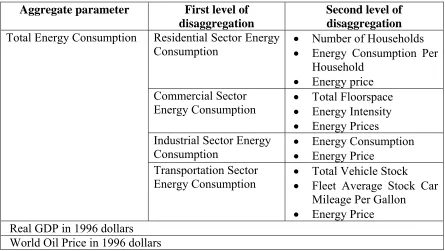
[image:22.612.84.529.464.715.2]The following table represents the EIA data used in this thesis:
Table 2 - Forecasted parameters used in analysis
Aggregate parameter First level of disaggregation
Second level of disaggregation Residential Sector Energy
Consumption • • Number of Households Energy Consumption Per Household
• Energy price Commercial Sector
Energy Consumption • • Total Floorspace Energy Intensity • Energy Prices Industrial Sector Energy
Consumption • • Energy Consumption Energy Price Total Energy Consumption
Transportation Sector
Energy Consumption • • Total Vehicle Stock Fleet Average Stock Car Mileage Per Gallon
• Energy Price Real GDP in 1996 dollars
For my analysis I built spreadsheets that contain data points for each sector, each
AEO and each year available, conversions needed for comparison and calculations of
percentage errors, absolute percentage errors, MPE, MAPE, and MSFPE.
Separate spreadsheets contain regression analyses with analysis of correlation
between errors in world oil prices and errors in prices of energy by sector, GDP errors
and energy consumption. I expect that errors in world oil price are having major impact
on accuracy of energy prices for transportation sector. Because higher levels of
production lead to higher energy consumption (given constant energy intensity) and
higher real GDP levels it is interesting to study how errors in real GDP influence errors in
energy consumption by sector.
Potential problems.
There are several potential problems with the data I used in my analysis. The first
problem is that there are only few data points to analyze for most recent AEO. For
example, for AEO 2003 actual data exists for only one year, two years for AEO 2002,
etc. This may introduce potential problems when analyzing if forecasts are getting better
over time.
Another problem appears with the analysis of forecasts with the longest
forecasting horizon. Both MPE and MAPE have a few data points, thus negating
smoothing properties of averaging. For example, for the forecasting horizon of 13-15
4.
Total energy consumption decomposition
Analysis of MAPE by Sector
This analysis offers a closer look at the general accuracy of forecasts, by sector,
for time horizons ranging from one to ten years. This analysis can be used to determine
if: (a) forecasts exhibit increased uncertainty when time horizons are lengthened; and (b)
certain sectors demonstrate a more accurate level of forecasting than others.
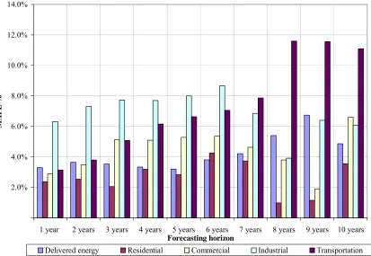
Table 3 presents both MAPE and MPE calculations by sector and in total. The
results from the MAPE analysis are shown in Figure 1. Figure 1 demonstrates that while
total energy consumption forecasts have relatively small errors for the time horizons
analyzed (ranging from 1.7% to 4.8%), the sectoral errors are much higher. In particular,
the transportation sector errors range from a low of 3.0% as an average for 1-year
forecasts, to over 11% for 8-, 9-, and 10-year forecasts. The most accurate forecasts seem
Table 3 - Energy Consumption Errors by Sector
Forecast horizon (years)
1 2 3 4 5 6 7 8 9 10 Number of
observations 14 14 12 11 11 8 6 4 2 3
MPE
Delivered energy 1.66% 1.58% 1.28% 0.77% 0.10% -0.94% -2.53% -5.40% -6.74% -4.86%
Residential 0.79% 0.11% -0.30% -1.47% -0.90% -3.27% -2.99% -0.72% 0.12% -1.71%
Commercial -0.44% -0.50% -0.69% -0.88% -2.31% -2.47% -2.07% -2.40% -1.87% -6.61%
Industrial 3.81% 4.84% 5.55% 6.00% 5.88% 5.51% 2.92% -2.30% -6.40% 0.41%
Transportation 0.57% -0.35% -1.66% -2.93% -4.50% -5.89% -7.87% -11.60% -11.56% -11.09%
MAPE
Delivered energy 3.30% 3.64% 3.53% 3.34% 3.20% 3.81% 4.21% 5.40% 6.74% 4.86%
Residential 2.37% 2.54% 2.06% 3.19% 2.83% 4.26% 3.74% 0.98% 1.15% 3.55%
Commercial 2.89% 3.47% 5.13% 5.09% 5.28% 5.35% 4.63% 3.80% 1.87% 6.61%
Industrial 6.32% 7.31% 7.71% 7.70% 8.00% 8.67% 6.86% 3.91% 6.40% 6.08%
Transportation 3.14% 3.80% 5.08% 6.16% 6.63% 7.05% 7.87% 11.60% 11.56% 11.09%
MSPFE
Delivered energy 1.66% 1.58% 1.28% 0.77% 0.10% -0.94% -2.53% -5.40% -6.74% -4.86%
Residential 0.11% 0.00% -0.06% -0.25% -0.15% -0.53% -0.49% -0.11% 0.02% -0.26%
Commercial -0.05% -0.06% -0.09% -0.12% -0.27% -0.30% -0.25% -0.27% -0.20% -0.73%
Industrial 1.35% 1.72% 1.97% 2.13% 2.09% 1.95% 0.98% -0.90% -2.46% 0.11%
Figure 1 - MAPE for Energy Consumption by Forecast Length
2.0% 4.0% 6.0% 8.0% 10.0% 12.0% 14.0%
1 year 2 years 3 years 4 years 5 years 6 years 7 years 8 years 9 years 10 years
Forecasting horizon
MAP
E
%
Delivered energy Residential Commercial Industrial Transportation
Analysis of MPE by Sector
This analysis expands on the MAPE analysis by identifying the directionality of
forecast error. That is, this analysis can be used to determine if certain sectors tend to
under-estimate or over-estimate forecast errors consistently for a certain time horizon.
This analysis might point to a systemic problem with the forecast models being used for a
given time horizon. The fact that the MAPE for total energy consumption is lower than
errors for individual sectors means that there is a cancellation of errors across energy
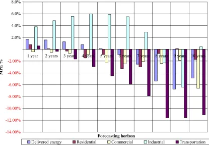
aspects of each sector’s energy forecasts. MPE calculations are shown in Table 3 and
Figure 2.
For forecasts of five years or less, total energy consumption errors are small on
average (around 1%) and are positive (representing overestimation). However, for
forecasts between 6-10 years in length, the errors are larger (about 4%) and are negative
(representing underestimation). The transportation sector is observed to be highly and
systematically underestimated, while the industrial sector tends to be overestimated,
[image:27.612.101.516.334.623.2]particularly for shorter forecast horizons.
Figure 2 - MPE for Energy Consumption by Forecast Length
-14.00% -12.00% -10.00% -8.00% -6.00% -4.00% -2.00%
2.0% 4.0% 6.0% 8.0%
1 year 2 years 3 years 4 years 5 years 6 years 7 years 8 years 9 years 10 years
Forecasting horizon
MP
E %
Delivered energy Residential Commercial Industrial Transportation
I apply the MSFPE discussed earlier to help partition out the sectoral
contributions of each sector on the total forecast error. Determination of sector error as a
function of total forecast error is important. Such analysis demonstrates sectoral
contributions to total error and helps us to determine if there are sectors in particular that
have “high leverage” with respect to total error.
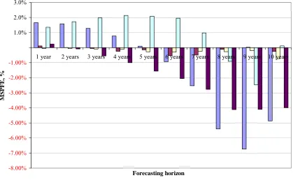
Table 3 shows MSFPE for each sector. Recall that MSFPE demonstrates a
sector’s average, real contribution to the total energy forecast error for a given forecast
length. As shown in Figure 3, the transportation sector is a major contributor to total
energy forecast error, particularly for forecasts with longer time horizons. In some cases,
transportation underestimation by itself exceeds the total forecast underestimation, since
the error is reduced by overestimation in other sectors. For forecasts with time horizons
Figure 3 - MSPFE for Energy Consumption by Forecast Length
-8.00% -7.00% -6.00% -5.00% -4.00% -3.00% -2.00% -1.00%
1.0% 2.0% 3.0%
1 year 2 years 3 years 4 years 5 years 6 years 7 years 8 years 9 years 10 years
Forecasting horizon
MS
P
F
E
, %
Analysis of Total Energy Consumption Forecast Improvements
For a given forecast horizon, error trends can be analyzed to determine if forecasts
are improving over time. For example, one may ask: Have 7-year forecasts improved in
accuracy from 1982 to 1996? I conduct this analysis for several forecast time horizons
(3-year, 5-(3-year, and 7-year) across sectors.
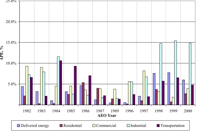
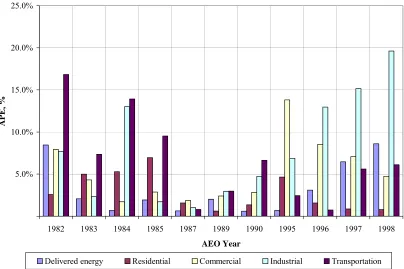
Figures 4 through 6 present the results of this analysis. Each graph shows the
absolute error based on the year in which the forecast was made. So, for example, Figure 4
evaluates whether three-year forecasts improved over time (from 1982-2000). Similarly,
using Figures 5 and 6, it can be determined whether five-year and seven-year forecasts
have improved.
The figures show that there is a general randomness, but it is interesting to note
that all graphs are bowl shaped with a minimum around AEO 1987 – AEO 1989. Errors
for this period look smaller. I see several reasons of such behavior. First is that period of
1987-1994 was relatively stable in terms of world oil prices (except for short period of
instability in 1990) thus making it easier to predict them. It can also be just a random
Figure 4 - Absolute Errors in Energy Consumption by Sector for Three-Year Forecasts by Year of
Forecast.
5.0% 10.0% 15.0% 20.0% 25.0%
1982 1983 1984 1985 1986 1987 1989 1996 1997 1998 1999 2000
AEO Year
AP
E,
%
Figure 5 - Absolute Errors in Energy Consumption by Sector for Five-Year Forecasts by Year of
Forecast
5.0% 10.0% 15.0% 20.0% 25.0%
1982 1983 1984 1985 1987 1989 1990 1995 1996 1997 1998
AEO Year
AP
E
, %
Figure 6 - Absolute Errors in Energy Consumption by Sector for Seven-Year Forecasts by Year of
Forecast
5.0% 10.0% 15.0% 20.0% 25.0%
1982 1983 1987 1989 1993 1996
AEO Year
AP
E
, %
Delivered energy Residential Commercial Industrial Transportation
Figure 7 shows actual energy consumption by sector for the period between 1980
and 2003. It is easy to notice that transportation, commercial and residential energy
consumption grew in a much more predictable way than industrial sector energy
consumption. Residential and commercial sectors energy consumption were growing
linearly without sudden boom and busts. Variability around the linear trend is small. In
case of the transportation sector the trend looks more like quadratic or exponential
equation. But still variability is small. The industrial sector energy consumption does not
show any strongly pronounced trend. Energy consumption has periods of growth and
Consistent growth of energy consumption in the residential, commercial and
transportation sector may suggest that it is easier to predict energy consumption for thsese
sectors. And indeed commercial and residential sectors energy consumption MPEs are the
lowest of the four. Transportation and industrial sector energy consumption MPE are the
highest and close to each other. It is not clear why predicting transportation sector energy
consumption is more difficult if compared to residential and commercial sectors. I’ll study
this problem in transportation sector analysis.
Figure 7 - Energy consumption by sector
0.00 5.00 10.00 15.00 20.00 25.00 30.00
1980 1982 1984 1986 1988 1990 1992 1994 1996 1998 2000 2002
Year
E
ne
rgy cons
um
pt
ion,
th
rill
ion btu
5.
Transportation sector analysis
As previous analysis showed, the transportation sector along with the industrial
sector are the most important sectors in terms of influence on total error. The
transportation sector is responsible for up to 82% of total error (Table 3). Unfortunately
before 1996 transportation sector data in AEO consisted of only transportation sector
energy consumption and energy price. After 1996 it also includes total vehicle-miles
traveled (VMT), average gas consumption in miles per gallon (MPG), and total fleet
stock. I used only data only for Light Duty Vehicles as they represent the largest portion
of transportation sector energy consumption. Data for air, rail and marine transportation
were not analyzed because of different representation that made comparison between
different types of transports impossible.
Analysis of Transportation Sector MPE and MAPE
To find how accurate U.S. transportation sector energy forecasts are I analyzed
MAPE and MPE for total energy consumption, total vehicle stock, total vehicle miles
traveled and transportation sector average energy price. As Table 3 shows, transportation
energy sector consumption error (MAPE) gradually grew from 3.14% for 1 year forecasts
to more than 11% for 8 and more years forecast. Another type of question to ask about
forecasts is how forecasts’ accuracy changing as one predict more and more distant events.
Given the unstable nature of the economy and complexity of societal interactions we can
intuitively assume that it is harder to predict further events.
Figure 8 and Figure 9 show how transportation sector energy consumption, total
NEMS behave over time. Transportation sector energy consumption and total vehicle
stock predictions were the least accurate and errors were growing fast, transportation
sector energy consumption and average MPG projections were the most accurate of all
projections. Because of very limited sample I was not able to explain why errors for fleet
average stock car MPG and total VMT average become smaller for longer projections.
It is easy to see that relatively small errors in sector energy consumption hide
larger errors in predicting sector specific parameters. In case of the transportation sector,
the total number of vehicles error is much greater than energy consumption error. Errors in
predicting energy price for transportation sectors, which will be analyzed separately later,
are even larger.
Figure 8 – Transportation sector MAPE for NEMS model
2.0% 4.0% 6.0% 8.0% 10.0% 12.0% 14.0% 16.0% 18.0% 20.0% 1 ye ar 2 ye ar s 3 ye ar s 4 ye ar s 5 ye ar s 6 ye ar s Forecast horizon MP E , %
Figure 9 – Transportation sector MPE for NEMS model
-10.00% -5.00% 5.00% 10.00% 15.00% 20.00% 25.00%
1 y
ear
2 y
ear
s
3 y
ear
s
4 y
ear
s
5 y
ear
s
6 y
ear
s
Forecast horizon
MP
E
, %
Total Vehicle Stock Total VMT Fleet Average Stock Car MPG Energy consumption
Analysis of the MPE graph (Figure 9) shows that total vehicle stock was
consistently overestimated, energy consumption underestimated, total VMT and Fleet
average MPG were predicted with good accuracy and errors do not tend to grow as
forecast horizon becomes longer.
Analysis of Transportation Energy Sector Forecast Improvements
To analyze how forecasts’ accuracy is changing over time I built graphs with errors
of 1 year forecasts, 2 year forecast, etc. Figure 10 and Figure 11 show a very typical view
for that sort of graph. Errors in energy prices dwarf all other errors; they behave
erratically. On the other hand errors in energy consumption show underestimation for
AEO published before 1996 and overestimation after that. In 1996 EIA switched from
change in errors behavior before 1996 and after troublesome. It is unclear if such changes
were mainly because of changes in the model or changes in assumptions. Overall I did not
find any accuracy improvement over time.
Figure 10 – Percentage error for 1-year forecast for transportation sector by AEO
-30.00% -20.00% -10.00% 10.00% 20.00% 30.00%
1983 1984 1985 1986 1987 1989 1996 1997 1998 1999 2000 2001 2002
AEO
Pe
rc
en
ta
ge
Error,
%
Total Vehicle Stock Total VMT Fleet Average Stock Car MPG
Figure 11 - Percentage error for 4-year forecast for transportation sector by AEO -30.00% -20.00% -10.00% 10.00% 20.00% 30.00% 40.00% 50.00% 60.00% 70.00% 80.00% AEO 1982 AEO 1983 AEO 1984 AEO 1985 AEO 1986 AEO 1987 AEO 1989 AEO 1996 AEO 1997 AEO 1998 AEO 1999 E rro r, %
Total Vehicle Stock Total VMT Fleet Average Stock Car MPG
Energy consumption Energy price
Analysis of Assumptions’ Influence on Transportation Energy Sector Forecast
Accuracy
Assumptions are important factors influencing every model. They "represent the
forecaster's basic outlook on the context within which the specific forecasted trend
develops" (Ascher, p. 199). Ascher thinks that assumptions are the most important
determinants of a forecast’s accuracy. The transportation sector uses numerous input
values (The Transportation Sector Model of the National Energy Modeling System, 2004,
p. 8). Among them are fuel prices, new vehicle sales, economic and demographic
price – which is a good encompassing indicator of fuel prices that are used in the
transportation sector; and GDP which is an indicator of economic performance and thus
influences many related variables.
Energy price errors for transportation sector are quite distinct among other errors
that I analyzed before. Figure 12 show MAPE for transportation sector energy
consumption and energy prices along with U.S. GDP and world oil prices for later
analysis. Because world oil price errors and energy price errors were much larger than all
other errors I plotted them on secondary axis. It is important to mention that last three
average values were obtained from only one observation. Errors in predicting energy
prices are so large that they cast doubt over the usefulness of such predictions. MAPE for
energy price goes as high as 232% for 12 years. Figure 13 show MPE for the same
parameters. Transportation sector energy price MPE shows that on average energy prices
were underestimated for up to 5 years forecasts and greatly overestimated after that.
As Figure 12 and Figure 13 show, world oil price MPE and transportation sector
energy price MPE are moving synchronously. They have very similar patterns and
behavior over time.
Figure 12 shows that transportation sector energy prices MPE reaches 232%, and
Figure 12 – Transportation sector energy price and energy consumption MPE, world oil price
and GDP MAPE
5.00% 10.00% 15.00% 20.00% 25.00% 30.00% 1 ye ar 2 ye ar s 3 ye ar s 4 ye ar s 5 ye ar s 6 ye ar s 7 ye ar s 8 ye ar s 9 ye ar s 10 ye ar s 11 ye ar s 12 ye ar s 13 ye ar s 14 ye ar s Forecast horizon MP E , % 50.00% 100.00% 150.00% 200.00% 250.00% 300.00% 350.00% 400.00% 450.00% 500.00% W or ld O il Pr ic e a nd Ene rgy pr ic e M A PE, %
Energy consumption GDP (1996$) Energy price (1996$) World Oil Price (1996$)
Figure 12 shows that transportation sector energy consumption, GDP, world oil
price and transportation sector energy price suffer from severe systemic errors. Both world
oil price and energy price were consistently overestimated, while energy consumption
underestimated. GDP projections tend to be underestimated for the first few years and
then overestimated. Amplitude of MAPE is smaller than MPE which means that some
cancellation of errors exists. If we consider the assumption that growing energy prices
decrease energy consumption by a certain degree (short and long term elasticity),
underestimation of the energy consumption can be partially explained by the
Figure 13 - Transportation sector energy price and energy consumption MAPE, world oil
price and GDP MPE
-30.00% -20.00% -10.00% 10.00% 20.00% 30.00% 1 y ear 2 y ears 3 y ears 4 y ears 5 y ears 6 y ears 7 y ears 8 y ears 9 y ears 10 y ears 11 y ears 12 y ears 13 y ears 14 y ears Forecast horizon MP E, % -500.00% -400.00% -300.00% -200.00% -100.00% 100.00% 200.00% 300.00% 400.00% 500.00% W or ld O il P ri ce an d E ner gy P ri ce M P E ,%
Energy consumption GDP (1996$) Energy price (1996$) World Oil Price (1996$)
To find if there is any relationship between world oil prices MPE and
transportation energy sector price MPE I used regression analysis. Figure 14 shows
distribution of energy price errors vs. world oil price errors and a linear trend line. The
regression equation is
Y=0.4844X+0.0788, where
Y – energy price MPE
X - world oil price MPE
R square is 0.97 which means that 97% of total variability of energy price MPE
line. Line slope of 0.4844 means that for approximately every two percent reduction in
world oil price MPE we can expect one percent reduction in energy price MPE.
Figure 14 – Transportation sector energy price errors vs. world oil price (1996$) errors for
forecasting horizon from 1 to 14 years
y = 0.4934x + 0.0423 R2 = 0.9724
50.00% 100.00% 150.00% 200.00% 250.00%
50.00% 100.00% 150.00% 200.00% 250.00% 300.00% 350.00% 400.00% 450.00% 500.00%
World oil price error, %
Ene
rgy pr
ic
e
(1
996$)
e
rr
or
, %
To analyze the possibility of reduction in world oil price errors I built a graph that
shows actual values of world oil price and forecasted with IFFS and NEMS. Figure 15
shows how world oil prices were predicted in different AEO in comparison with actual
values. All forecasts show gradual smooth increase in oil prices, while actual values show
very different behavior.
Figure 16 shows how world oil prices were changing over the period between 1974
Figure 16 is a good confirmation of his words “nothing appears to be more
incorrect where the future of oil prices is concerned than charting largely horizontal lines”.
Figure 15 shows typical, what William Ascher (Ascher, 1978) calls it, “assumption drag”,
when changing trends are not captured in forecasts and forecasters continue using
outdated and incorrect assumptions. AEO produced in 1982, 1983, 1984, 1987, and 1989
are greatly overestimating world oil prices and forecasting rapid growth of oil prices over
time even when prices started to fall.
During periods of high and growing oil prices both models forecasted rapid, almost
exponential growth in the future. Periods of stable world oil prices tend to flatten forecasts
to a gradual growth.
For periods of relatively stable oil prices linear trends appear to be the best
estimate of future oil prices and NEMS forecasts made in 1996-2003 are more precise
than earlier projections. This precision is attributed only to stable prices and any random
shocks in the nearest future will reduce accuracy. Taking into account random nature of
world oil prices it is unrealistically to expect world oil price forecasts along with
Figure 15 – Comparison of actual and forecasted world oil prices (AEO 1982-2004)
10.0 20.0 30.0 40.0 50.0 60.0 70.0
1980 1985 1990 1995 2000 2005
Year
P
ri
ce,
1
99
6$
1982 1983 1984 1985 1986 1987 1989 1990 1992 1994 1995 1996 1997 1998 1999 2000 2001 2002 2003 2004 Actual
Figure 16 – World oil prices chronology (World Oil Market and Oil Price Chronologies: 1970 – 2004)
0.00 10.00 20.00 30.00 40.00 50.00 60.00 70.00
Jul-72 Jan-78 Jul-83 Dec-88 Jun-94 Dec-99 May-05 Period
O
il
Pr
ic
e,
1
Another important assumption for both IFFS and NEMS is GDP. In contrast to
world oil prices, GDP grows in a quite predictable manner without sudden booms and
busts over time (Figure 17). But even for such forecasting is not particularly accurate and
errors go as high as 25% (Figure 12). Because GDP is behaving in such predictable way I
decided to do forecasting using regression analysis techniques. Table 4 shows the results
of such analysis. I used historical real GDP in billions of 2000 dollars from 1970 to 1994
to build an exponential growth model. Then I forecasted real GDP for 1995-2003 using
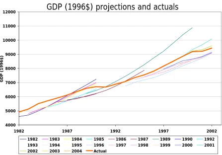
this model and compared these forecasts with actual data. Column (6) percent error shows
that for period of 9 years error didn’t exceed 4% which is better than results received with
much more complex IFFS and NEMS models shown in Figure 18.
Figure 17 - Real GDP chronology and forecasting results
0.0 2,000.0 4,000.0 6,000.0 8,000.0 10,000.0 12,000.0
1970 1975 1980 1985 1990 1995 2000 Year
G
D
P
, b
illion
s of
c
h
ain
e
d
2000 d
o
llars
Table 4 - GDP exponential trend calculation
Year GDP in
billions of chained 2000 dollars Linearized GDP Forecasted linearized GDP Forecasted GDP (exponential growth) Percent Error
(1) (2) (3) (4) (5) (6)
1970 3,771.9 8.2353 8.250 3827.5 1.47%
1971 3,898.6 8.2684 8.280 3944.2 1.17%
1972 4,105.0 8.3200 8.310 4064.4 -0.99%
1973 4,341.5 8.3760 8.340 4188.3 -3.53%
1974 4,319.6 8.3709 8.370 4316.0 -0.08%
1975 4,311.2 8.3690 8.400 4447.6 3.16%
1976 4,540.9 8.4209 8.430 4583.1 0.93%
1977 4,750.5 8.4660 8.460 4722.8 -0.58%
1978 5,015.0 8.5202 8.490 4866.8 -2.96%
1979 5,173.4 8.5513 8.520 5015.2 -3.06%
1980 5,161.7 8.5490 8.550 5168.0 0.12%
1981 5,291.7 8.5739 8.580 5325.6 0.64%
1982 5,189.3 8.5543 8.610 5487.9 5.76%
1983 5,423.8 8.5985 8.640 5655.2 4.27%
1984 5,813.6 8.6680 8.670 5827.6 0.24%
1985 6,053.7 8.7084 8.700 6005.2 -0.80%
1986 6,263.6 8.7425 8.730 6188.3 -1.20%
1987 6,475.1 8.7757 8.760 6376.9 -1.52%
1988 6,742.7 8.8162 8.790 6571.3 -2.54%
1989 6,981.4 8.8510 8.820 6771.6 -3.00%
1990 7,112.5 8.8696 8.851 6978.1 -1.89%
1991 7,100.5 8.8679 8.881 7190.8 1.27%
1992 7,336.6 8.9006 8.911 7410.0 1.00%
1993 7,532.7 8.9270 8.941 7635.9 1.37%
1994 7,835.5 8.9664 8.971 7868.6 0.42%
1995 8,031.7 8.9911 9.001 8108.5 0.96%
1996 8,328.9 9.0275 9.031 8355.7 0.32%
1997 8,703.5 9.0715 9.061 8610.4 -1.07%
1998 9,066.9 9.1124 9.091 8872.8 -2.14%
1999 9,470.3 9.1559 9.121 9143.3 -3.45%
2000 9,817.0 9.1919 9.151 9422.0 -4.02%
2001 9,866.6 9.1969 9.181 9709.2 -1.60%
2002 10,083.0 9.2186 9.211 10005.2 -0.77%
Figure 18 – Comparison of actual and forecasted real GDP values
GDP (1996$) projections and actuals
4000 5000 6000 7000 8000 9000 10000 11000 12000
1982 1987 1992 1997 2002
Year
G
D
P
(199
6$
)
1982 1983 1984 1985 1986 1987 1989 1990 1992 1993 1994 1995 1996 1997 1998 1999 2000 2001 2002 2003 2004 Actual
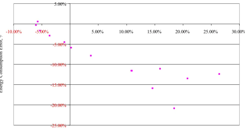
Figure 19 shows that GDP and energy consumption errors are somehow related,
and improvement of GDP accuracy will influence energy consumption accuracy. The
graph shape is not exactly linear as in case of world oil prices and transportation sector
energy prices but it shows that higher by absolute value errors in GDP lead to higher by
Figure 19 – Transportation sector energy consumption errors VS GDP errors for 1 to 14
years forecast
-25.00% -20.00% -15.00% -10.00% -5.00% 5.00%
-10.00% -5.00% 5.00% 10.00% 15.00% 20.00% 25.00% 30.00%
GDP error, %
E
ne
rgy
Cons
um
pt
ion
Er
ro
r,
%
NEMS documentation states: “Four end-use demand modules represent fuel
consumption in the residential, commercial, transportation, and industrial sectors, subject
to delivered fuel prices, macroeconomic influences, and technology characteristics.” (The
National Energy Modeling System: An Overview 2003). Fuels that are used in the
transportation sector are mainly petroleum based. Because of this, fuel prices depend very
much on world oil prices. So, high error in predicting transportation sector energy price
may introduce additional error in predicting energy consumption. Figure 20 presents a
graph of transportation sector energy consumption MPE vs energy price MPE. The graph
shows that generally high overestimation of world oil prices lead to underestimation of
energy consumption. The link between energy consumption and energy price in
Figure 20 - Transportation sector energy consumption MPE vs energy price MPE
-14.00% -12.00% -10.00% -8.00% -6.00% -4.00% -2.00%
2.00%
10.00% 20.00% 30.00% 40.00% 50.00% 60.00% 70.00% 80.00% 90.00% 100.00%
Energy price MPE
E
ne
rg
y co
ns
umption M
6.
Industrial sector analysis
The manufacturing sector consists of all manufacturing establishments in the 50
States and the District of Columbia (Energy Use in Manufacturing, 2005).
The industrial sector is similar to the transportation sector by the impact it has on
error in total energy consumption (Table 3). While errors in energy consumption in the
transportation sector are slowly growing over time, errors in the industrial sector energy
consumption (MPE) have a wavy form that show slow growth in the beginning and slow
decay at the end (Figure 21). This form can be explained by initial positive bias and
underestimated growth rate. The similarity of MPE and MAPE for the first six years
shows that energy consumption for industrial sector was generally overestimated, and
after that both overestimation and underestimation exist. It is also interesting to note that
for up to 10 years there is no visible growth in the amplitude of MPE or MAPE which
Figure 21 - MPE and MAPE for industrial sector energy consumption
-9.00% -7.00% -5.00% -3.00% -1.00% 1.00% 3.00% 5.00% 7.00% 9.00% 11.00%
1 year 2 years 3 years 4 years 5 years 6 years 7 years 8 years 9 years 10 years
MPE MAPE
Errors in predictions of energy prices are very similar in behavior to those of the
transportation sector. Industrial sector energy prices are overestimated and the degree of
overestimation is rapidly growing over time. MPE and MAPE are very close to each other
which means that there is no cancellation of errors and energy price accuracy suffer from
Figure 22 - MPE and MAPE for industrial sector energy price
-20.00% 20.00% 40.00% 60.00% 80.00% 100.00% 120.00% 140.00% 160.00%
1 year 2 years 3 years 4 years 5 years 6 years 7 years 8 years 9 years 10 years
MPE MAPE
Analysis of Industrial Energy Sector Forecast Improvements
Figure 23, Figure 24, and Figure 25 show errors in forecasting industrial sector
energy consumption and energy prices for 3, 5 and 7 years forecasts respectively. These
figures help to analyze how forecasts’ accuracy was changing between AEOs. Analysis of
energy consumption shows that there are no signs of improving accuracy over time.
Switching from IFFS to NEMS in 1996 did not improve accuracy. At the same time
energy prices accuracy improved to some degree. This improvement in accuracy can be
attributed to relatively more stable prices over the period of 1990-2003 if compared to pre
1990 period. But because improvements in accuracy are mainly attributed to a stable
environment I do not expect it to improve further. The next random shock can reverse
Figure 23 - Errors in 3 years forecasts of industrial sector energy consumption and energy price -30.00% -20.00% -10.00% 10.00% 20.00% 30.00% 40.00% 50.00% 60.00% 70.00% AEO 1982 AEO 1983 AEO 1984 AEO 1985 AEO 1986 AEO 1987 AEO 1989 AEO 1996 AEO 1997 AEO 1998 AEO 1999 AEO 2000
Energy consumption Energy price
Figure 24 - Errors in 5 years forecasts of industrial sector energy consumption and energy price
-40.00% -20.00% 20.00% 40.00% 60.00% 80.00% 100.00% 120.00% 140.00% AEO 1982 AEO 1983 AEO 1984 AEO 1985 AEO 1987 AEO 1989 AEO 1990 AEO 1995 AEO 1996 AEO 1997 AEO 1998
[image:54.612.98.527.431.647.2]Figure 25 - Errors in 7 years forecasts of industrial sector energy consumption and energy
price
-40.00% -20.00% 20.00% 40.00% 60.00% 80.00% 100.00% 120.00% 140.00% 160.00% 180.00%
AEO 1982 AEO 1983 AEO 1987 AEO 1989 AEO 1993 AEO 1996
Energy consumption Energy price
Analysis of Assumptions’ Influence on Industrial Energy Sector Forecast Accuracy
Figure 26 and Figure 27 show results of an analysis of the influence of errors in
core assumptions on accuracy of industrial sector energy consumption and energy price.
These figures are very similar to the figures presented for the transportation sector. Higher
MPE in predicting world oil prices leads to higher MPE in predicting industrial sector
energy prices. The relationship is quite linear and line slope suggests that for each percent
improvement in world oil price MPE we can expect 0.65% improvement in industrial
Figure 26 - Industrial sector energy price MPE vs. world oil price (1996$) MPE
y = 0.6504x + 0.0733 R2 = 0.945
-50.00%
50.00% 100.00% 150.00% 200.00% 250.00% 300.00% 350.00%
50.00% 100.00% 150.00% 200.00% 250.00% 300.00% 350.00% 400.00% 450.00% 500.00%
World oil price error, %
E
ne
rgy pr
ic
e (
199
6$
)
er
ro
r,
%
Figure 27 shows relationship between industrial sector energy consumption MPE
and real GDP MPE. Relationship is not readily visible but we can assume that increased
Figure 27 - Industrial sector energy consumption MPE vs. GDP MPE
-20.00% -15.00% -10.00% -5.00% 5.00% 10.00%
-10.00% -5.00% 5.00% 10.00% 15.00% 20.00% 25.00% 30.00%
GDP error, %
E
ne
rgy C
ons
um
ptio
n E
rr
or
, %
7.
Commercial sector analysis
The commercial sector consists of business establishments and other organizations
that provide services. The sector includes service businesses, such as retail and wholesale
stores, hotels and motels, restaurants, and hospitals, as well as a wide range of buildings
that would not be considered “commercial” in a traditional economic sense, such as public
schools, correctional institutions, and religious and fraternal organizations. Excluded from
the sector are the goods-producing industries: manufacturing, agriculture, mining, forestry
and fisheries, and construction (Background Information on CBECS, 2001).
The commercial sector is number three by its influence on total energy
consumption accuracy. The commercial sector energy consumption MAPE fluctuates
between 3% and 7%. At the same time MPE is always negative and smaller by absolute
value (Figure 28). This means that there is a slight negative bias in forecasting energy
[image:58.612.102.524.506.708.2]consumption for the commercial sector.
Figure 28 - Commercial sector energy consumption MPE and MAPE
-9.00% -7.00% -5.00% -3.00% -1.00%
1.00% 3.00% 5.00% 7.00% 9.00% 11.00%
1 year 2 years 3 years 4 years 5 years 6 years 7 years 8 years 9 years 10 years
The commercial sector energy prices were almost always overestimated and errors
in predicting energy prices grow rapidly over time. MAPE grows from less then 10% for 1
year forecast to more than 70% in 10 years forecast (Figure 29). MPE is either slightly less
than MAPE or equal to it which means that periods of underestimation exist but they are
not reversing general overestimation trend.
Figure 29 - Commercial sector energy price MPE and MAPE
-10.00%
10.00% 20.00% 30.00% 40.00% 50.00% 60.00% 70.00% 80.00%
1 year 2 years 3 years 4 years 5 years 6 years 7 years 8 years 9 years 10 years
Energy price MPE Energy price MAPE
Figure 30 and Figure 31 show results of MAPE and MPE analys