An Evaluation Of A Multigrid Algorithm Error Spike Correction Method

Rochester Institute of Technology

RIT Scholar Works

Theses

Thesis/Dissertation Collections

2005

An Evaluation Of A Multigrid Algorithm Error

Spike Correction Method

Erika L. McMichael

Follow this and additional works at:

http://scholarworks.rit.edu/theses

This Thesis is brought to you for free and open access by the Thesis/Dissertation Collections at RIT Scholar Works. It has been accepted for inclusion

in Theses by an authorized administrator of RIT Scholar Works. For more information, please contact

[email protected].

Recommended Citation

An Evaluation Of A Multigrid Algorithm Error

Spike Correction Method

by

Erika L. McMichael

A

Thesis Submitted

in

Partial Fulfillment

of the

Requirements for the Degree

of

Master

of Science

in Mechanical Engineering

Approved

By:

Dr.

Amitabha

Ghosh

Department

of Mechanical

Engineering

Dr.

Ali

Ogut

Department

of Mechanical

Engineering

Dr. P. Venkataraman

Department of

Mechanical

Engineering

Dr

.

Edward

C.

Hensel

Mechanical

Engineering Department Head

Department

of

Mechanical Engineering

Rochester Institute

of

Technology

Thesis Release Permission Form

Rochester Institute of Technology

Kate Gleason College of Engineering

Title: An Evaluation Of A Multigrid Algorithm Error Spike Correction

Method

I, Erika L. McMichael, hereby grant permission to the Wallace Memorial Library to

reproduce my thesis in whole or in part. Any reproduction will not be for commercial

use or profit.

Erika

L.

McMichael

Erika L. McMichael

Copyright

2005

by

Erika L. McMichael

Acknowledgments

I

wish

to

thank

my advisor,

Dr.

Ghosh,

for his

guidance and support

in

completing

Abstract

This

study

is

an evaluation of a method of

improving

the

multigrid process

by

cor

recting

error spikes which are generated when

moving

from

a coarser

to

finer level.

The

correction method was

tested

on nine one-dimensional problems governed

by

second order

differential

equations.

Tests

were performed with an

accomodative,

full

approximation

scheme,

full

multi-grid algorithm.

Results indicate

that

appropriate

implementation

of

the

correction can

increase

so

lution

accuracy.

Accuracy

was

increased

in

75%

of cases

in

which a single correction was applied

to

a point

in the

central portion of

the

grid.

Single

corrections performed

on points with error greater

than the

average error were effective

86%

of

the

time.

Contents

Acknowledgments

iv

Abstract

v

1

Introduction

1

2

Computational Fluid Dynamics

3

3

Multigrid

6

3.1

Basic Multigrid Process

7

3.2

Multigrid

Algorithms

7

4

Multigrid Program

9

4.1

Basic

Elements

9

4.2

User Inputs

10

4.3

Structure

10

4.4

Convergence

Testing

11

4.5

Program

Outputs

12

4.6

Program

Efficiency

12

5

Correction

Method

14

5.1

Description

of

Correction

14

5.2

Correction

Processing

Time

16

6

Problems

17

7

Methods

19

8

Results

and

Discussion

21

8.1

Error Spike Direction

21

8.3

Point in Multigrid Cycle

25

8.4

Grid Location

27

8.5

Residual Magnitude

28

8.6

Problems

28

8.7

Multiple

Corrections

32

9

Conclusions

33

Bibliography

35

A Multigrid Program

-

Fortran 90

Code

36

A.l

Multigrid

-main.for

36

A. 2

Correction

44

A.3

Gauss Seidel

-gs.for

45

A. 4

Prolongation

and

Restriction

Operators

- _prores.for

47

B

Efficiency

Test

Programs

-

Fortran 90 Code

49

B.l

Gauss Seidel

Efficiency

Test Program

49

B.2

Correction

Efficiency

Test Program

52

C

Accomodative Algorithm Runs

56

D Multiple

Correction Results

61

List

of

Figures

2.1

Example

grid

5

3.1

Error

vs.

Grid Point: After initial

guess,

After 1 GS

iteration,

After

4

GS iterations

6

5.1

Problem

5,

Iteration

14.

Residual

vs.

Grid Point

(left)

and

Error

vs.

Grid Point

(right)

15

5.2

Problem

5,

Iteration

14.

Error

vs.

Grid Point

after replacement of

point

5

15

5.3

Error

vs.

Grid Point

one

GS

iteration

later

without

(left)

and with

(right)

correction

15

7.1

Generic

multigrid structure

20

8.1

Error

vs.

Grid

Point,

"Correct" spike

(left)

and "Incorrect" spike

(right)

22

8.2

Error

vs.

Grid

Point, "Partially

Correct" spike

22

8.3

Error

plot

(top)

and residual plot

(bottom)

for Problem

1,

Trial 1

(level

3)

24

8.4

Generic

multigrid

structure,

grid

level

vs. point

in

cycle

25

8.5

Change in

error vs. point

in

multigrid cycle

26

8.6

Change in final

error vs. correction

location

and

level

27

8.7

Change

in

final

error vs. residual/residual norm

29

8.8

Change

in

final

error vs. correction

location

and problem

30

List

of

Tables

4.1

Size

of computational

domain

per grid

level

10

4.2

Number

of

iterations

required

for

convergence

13

5.1

Work

required

for

a correction compared

to

a

Gauss Seidel iteration.

16

6.1

Problems

17

8.1

Percentage

of

trials

error was

decreased

or

increased

per error spike

direction

23

8.2

Average

percentage change

in

error per error spike

direction

23

8.3

Average

change

in

error per grid

level

24

8.4

Average

percentage change

in

error per

location

in

multigrid cycle. .

26

8.5

Number

of

trials

in

which

final

error was

increased

or

decreased

vs.

Chapter

1

Introduction

Multigrid is

an

iterative

method whichutilizes gridsofmultiple sizes

to

reduce error on

multiplewavelengths.

Many

classical

iterative

methods

(Gauss

Seidel,

etc.)

efficiently

reduce

the

error of

high

frequency

components,

"smoothing"

the

error.

Multigrid

uses a relaxation scheme

to

smooth

the

error on severalgrid

levels

of

varying

coarseness.

In

this way,

multigrid can

greatly

reduce

the time

required

to

obtain asolution.

Brandt

introduced

multigrid methods

in

his 1977

paper

[1].

Since

that time

several

books

have been

written on

the

topic,

including

[6], [5], [3],

and

[4].

In

this study the

multigrid process was examined

graphically through

plots of

the

residuals and error after each

iteration in

the

multigrid cycle.

From

the

examination

of

these

plots

it became

apparent

that

spikes

in

the

residual plots corresponded

to

spikes

in the

error plots.

It

was also noted

that

error spikes were prevalent when

moving to

finer

grid

levels.

A

correction method

designed

to

mitigate

these

error

spikes

is

described in

this

thesis.

Testing

showed

that the

removal of a single error

spike could

increase the accuracy

of

the

solution while

only

minimally

increasing

the

amount ofcomputational work.

To

evaluate

the

effectivenessof

the

correction

method,

a multigrid program was writ

ten

and nine one-dimensionalproblems were

tested.

The

multigrid program utilized

an

accomodative,

full

approximation

scheme,

full

multi-grid algorithm

(FAS

FMG).

Brandt

provides a

detailed description

of an accomodative

FAS FMG

algorithm

in

[2].

One-dimensional

problems were used

for

simplicity.

For

consistency, the

prob

lems

evaluated were allsecond order

differential

equations.

The differential

equation

solutions

include

five

polynomials, three trigonometric

functions,

and one exponential

function. The

effects ofseveral

independent

variables

(such

as grid

level,

location

on

grid,

etc.)

on solution

accuracy

and number of

iterations

required

for

convergence

were recordedand are presented

here.

A brief

introduction to

computational

fluid dynamics

(CFD)

is

given

in

Chapter

2

of

this

thesis.

The basic

multigrid process

is

outlined

in

Chapter

3,

and

the

multi-grid program used

in

this study

is

described in Chapter 4. Chapter 5 describes

the

implementation. The

problems used

in the study

are presented

in

Chapter

6.

Testing

Chapter

2

Computational Fluid

Dynamics

Many

fluid flow

problems cannot

be

solved analytically.

These

problems can

be

solved

numerically using

computation

fluid dynamics. Computational fluid dynamics

(CFD)

is

the term

given

to

a

variety

of numerical mathematical

techniques

used

to

solve

the

equations

that

govern

fluid flows

and aerodynamics.

CFD

was

developed in

the

1970s

after

the

introduction

of

high

speedcomputers.

Because

CFD

solvers use numerical methods

to

obtain a

solution, the

region

being

analyzed must

be divided

into

a gridwith

discrete

grid points.

A

numerical solution

is

obtained at each of

the

grid points.

To

use

CFD

to

solve a

problem, the

govern

ing

equations must

be discretized

so

that

the

values of

the

variables are considered at

the

grid point only.

If

there

are n grid points on

the grid,

n algebraic equations are

developed

by

discretizing

the governing

differential

equations.

Several discretiza

tion

schemes exist.

In

this

thesis,

differential

equations were

discretized

using

central

differencing

derived

from

the

Taylor

series expansion

(5.1),

(5.

2).

Other

types

of

dis

cretization

include

forward

and

backward

differencing

as well as

forward, backward,

or central

differencing

using

a

larger

number of grid points

(for

example

three

and

four

point

formulae).

When

a problem

is discretized it

changes

from

a

differential

equation

to

a set of algebraic equations.

If

the

problem

is

nonlinear

it

must

be linearized before it

can

be

solved

using the

methods

described in

this

thesis.

For

simplicity, only

linear

problems are

discussed

in this

thesis.

If

the

set of equations

is

linear it

can

be

represented

in

matrix

form

as:

Au

=

f

(2.1)

where,

A is

the

known

coefficient

matrix,

u

is

the

vector of n

dependent

variables,

and

/

is

the

vector of

known

values.

Equation

(2.1)

can

be

solved

using

direct

or

iterative

methods.

Direct

methods use a

finite

number of operations

to

obtain a solution and

iterative

methods use a variable numberof

iterations

depending

on

the

accuracy desired.

The

number of

iterations is

controlled

by

the stopping criteria,

usually

an average of

the

residuals

(the

difference between

/

and

Au

at each point).

Seidel iteration is

given

in

equation

(4.1).

Boundary

conditions are specified conditions on

the

edgesof

the

domain

which aid

in

the

solution of partial

differential

equations.

Common

boundary

condition

types

are

Dirichlet, Neumann,

and

Cauchy

boundary

conditions.

Dirichlet

boundary

conditions

specify the

values of

the

function

on

the

boundary.

Neumann

boundary

conditions

specify the

derivative

of

the

function

on

the

boundary.

Cauchy boundary

conditions

specify

a weighted average of

Dirichlet

and

Neumann

boundary

conditions.

When

Neumann

boundary

conditions are specified

the

boundary

conditions are part of

the

computational

domain

(the

computational

domain is

the

area of

the

grid where

the

values of

the

dependent

variable are

unknown)

.

Boundary

grid points with

Dirichlet

boundary

conditions are not

included in

the

computational

domain.

The

following

example

illustrates

the

process of

discretizing

the

partial

differential

equation

(2.3)

and

expressing

it in

the

matrix

form

Au

=

f

(2.6).

The

example applies

the steady

state

heat

conduction equation

(Laplace

equation)

(2.2)

to

a plate

with an unknown

temperature

distribution,

known

edge

temperatures,

and no

heat

generation.

In

(2.2)

u

is

the temperature

(the

dependent variable)

and

the

dimensions

of

the

plate are

Lx

L. The

temperature

is

constant

along

each edge of

the

plate.

The

temperatures

on

the

edges of

the

plate are

the

boundary

conditions and are

designated

Bi, B2, B3,

B4. For

example,

u =

B\

at x =

0

_{and u} =

B2

_at

y

=

L. The

_example

has Dirichlet

boundary

conditions

(known

boundary

values)

.

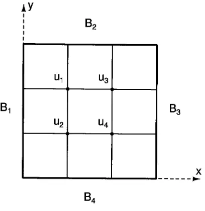
The

2-dimensional

plate

being

analyzed

is

shown

divided into

a grid

in

Figure

2.1.

The

distance between

grid points

in the

x and

y

directions

are

denoted

by

Ax

and

Ay

respectively.

In

this

case

Ax

=

Ay

= _~.

There

_are

four

_points

in the

_{computational}

domain

(n

=

4)

which are

labeled

u\, u2, u3,

and u^.

The

grid coordinates are

denoted

by

{i,j).

d2u

d2u

^

+

^=0

<2-2>

Ax2 Ay2

ui+1J

+

Uj_ij

-Auid

+

UiJ+1

+

Ujj-i

=

0

(2.4)

Grid

point

(f

,

^):

u3

+

Bx

-Am

+

B2

+

u2

=

₀

Grid

point

(f

,

f

):

u4

+

Bj

-Au2

4-m

+

BA

=

0

Grid

point

{f,

f):

B3

+

Ul

-Au3

+

B2

+ uA

=

0

{Lb)

Grid

point

(^,

f

):

B3

+

u2

iY

B,

B,

Ui

u3

u2

u4

B,

[image:15.533.115.319.77.287.2]

B.

Figure 2.1: Example

grid.

-4

1

1

0

i

_B\

B2

1

-4

0

1

u2

_Si

J94

1

0

-4

1

U3

B3

B2

0

1

1

-4

Ui

B3

?4

Chapter

3

Multigrid

Multigrid

methods are

iterative

methods used

to

solve partial

differential

equations.

Mulitgrid

methods use multiple grids of

varying

coarseness

to

speed

up

convergence.

The

two

main components of multigrid methods are error

smoothing

and coarse grid

correction.

Each

grid used

in solving the

problem

is identified

by

a grid

level

(for

example

the

coarsestgrid

is

referred

to

as

level

1).

On

eachgrid

level

the

error

is

"smoothed"

with

the

one or more

iterations

of a relaxation scheme

(e.g.

Gauss-Seidel)

.

The

relaxation

methods are efficient at

reducing the

error

(4.9)

of

high

frequency

components.

Figure

3.1

shows

the

effects of one and

four Gauss-Seidel iterations

on a one

dimensional

problem.

The high

frequency

errors are

quickly

resolved

giving the

plot a smooth

appearance.

Figure

3.1:

Error

vs.

Grid Point: After initial

guess,

After

1

GS

iteration,

After

4

GS

iterations.

Once

the

error on

the

fine

grid

is

smoothed

it is

transferred to

a coarser grid.

The

error

is

smoothed on

the

coarse grids and

the

coarse grid approximations are used

to

correct

the

finest

grid approximation.

Applying

the

relaxation scheme

to

grids of [image:16.533.63.471.418.527.2]

3.1

Basic Multigrid

Process

This

section

describes

the

multigrid process

in very

general

terms.

A detailed

descrip

tion

of

the

algorithm used

in this study

is

given

in the

next chapter.

The discretized

equation

to

be

solved

is

(2.1).

On

the

kth grid

level

the

discretized

equation

is

repre

sented as:

Akuk = fk

(3.1)

Restriction

and prolongation operators are used

to

move

between

grid

levels.

Re

striction operators are used

to transfer to

coarser

levels

and either

directly

inject

or

average

fine

grid values

to

obtain a coarse grid value.

Prolongation

operators use

interpolation

to transfer to

finer

grids.

The

restriction and prolongation operators

are

denoted

by

R

and

P

respectively.

Ruk+1 =

uk

(3.2)

Puk

= uk+1

(3.3)

The

first

step

in

the

multigrid process

is

presmoothing, the

application of v\

iterations

of an appropriate relaxation scheme.

This is

denoted by:

S(uk,Ak,fk,Vl)

(3.4)

The

process

then

moves

to

a

lower

(coarser)

grid

level.

On

the

lower

grid

level,

fk

is

modified and a relaxation scheme

is implemented

to

approximateuk

(3.1).

This

coarse

grid approximation

is

used

to

correct

the

finer

grid approximation.

The

value of fk

and

the meaning

ofuk

depend

on

the

multigrid scheme

(see

Coarse Grid

Processing,

below).

The

final

step

of

the

process

is postsmoothing,

relaxation on

the

fine

grid

level. These

steps can

be

performed multiple

times

on

any

number of grid

levels.

3.2

Multigrid

Algorithms

Starting

Point

Full Multi-Grid

(FMG)

algorithms

begin

on

the

coarsest

level

and move up.

The

coarsest

level

solution

may

be

obtained

by

relaxation or a

direct

method.

[2]

Cycling

algorithms

begin

with an approximation on

the

finest

grid.

The

approxima

tion

can

be

trivial,

such as u =

Program Progression

An

algorithm

is

described

as accomodative or

fixed.

Accomodative

algorithms use

internal

checks

to

determine

when a switch will

be

made

to

a

finer

or coarser

level.

The

checks are

usually

based

on relative magnitudes ofresiduals.

Fixed

algorithms

have

no

internal

checks and operate

based

on a predetermined

flow.

Fixed

algorithms

may

execute more

quickly than

accomodative algorithms

because

they

do

not require

the

calculation ofresiduals after each

iteration.

Coarse Grid

Processing

A

multigrid algorithm can use

the

Correction Scheme

or

the

Full

Approximation

Scheme described

in this

section.

In

the

Correction Scheme

the

long

wavelengtherror

of

the

fine

grid approximation

{uk+1)

is

approximated on

the

coarse grid

by

uk.

On

the

coarse

grid, the

right

hand

side ofequation

(3.1)

is

given

by

(3.6),

the

restriction

of

the

fine

grid residual error (rfc+1

(3.5)).

To

correct

the

fine

grid approximation

{uk+1),

uk

is

prolongated and added

to

uk+1

(3.7).

[2]

rk+1

= fk+l

-Ak+1uk+1

(3.5)

fk

= Rrk+i

(3>6)

E2

=

<u

+

Puk

(3.7)

In

the

Full

Approximation Scheme

(FAS)

the

coarse grid approximation

(uk)

approx

imates

the

solution

to the

differential

equation on

level k.

When

transferring

to

a

coarser

level

k,

an

initial

value ofuk

is

the

restriction ofuk+1

(3.8).

This

initial

value

is

used

in

the

calculation offk

(3.9).

The

fine

grid

is

corrected with

(3.

10).

[2]

uk

= Ruk+1

(3.8)

fk

= Akuk

+

Rrk+i

^

=

uk+}

+

P{uk-Ruktl})

(3.10)

ufe+i

new

The

algorithm used

is

fully

described

by

one

item

from

each of

the

above

three

sections.

The

program used

in

this study

is

an

accomodative,

full

approximation

Chapter

4

Multigrid Program

A

multigrid programwritten

for

this study

is described in

this

section.

This

program

provided a means of

testing

the

correction method.

The

program uses an accomoda

tive

full

approximation scheme

full

multi-grid

(FAS

FMG)

algorithm.

It is

capable of

solving

one

dimensional

problems with

Dirichlet

boundary

conditions.

The

program

source code

is in

Appendix A.

4.1

Basic Elements

Smoothing

Method

The Gauss-Seidel iteration is

used

for

error

smoothing

on all grid

levels. For

the

case

of

M

equations

the

n

+

1th round of

Gauss-Seidel

iterations

can

be

written as:

<+1

=

T

t-1 M

j=l j'=i+l

for

i

=

1

to

M

(4.1)

Gauss-Seidel

iterations

are performed

by

the

subroutine

gs.for,

see

Appendix A.

3.

Prolongation/Restriction

Operators

The

restriction and prolongation operators used

in

grid

transfer

are

defined

by

the

following

equations:

Ruj

=

-~u2j-i

+

7-U2J

+

~7u2j+i

Restriction

(4.2)

Pu2j

=

Uj

Pu2j+\

=

~{uj

+

Uj+i)

Prolongation

(4.3)

Zi

These

are

taken

from

[6].

Prolongation

and restriction matrices are created

in

the

Coefficient

Matrix

The finest level

coefficient matrix

A from

(2.1)

is

provided

by

the

user.

To

perform

smoothing

operations on all grid

levels,

an

A

matrixmust

be

obtained

for

each

level.

Here

the

Galerkin

coarse grid approximation

is

used:

Ak

=

RAk+ip

(44)

4.2

User

Inputs

Seven items

must

be

supplied

by

the

user

for

the

program

to

operate:

1.

nm

The

number of grid points

in

the

computational

domain

on

the

finest

level

2.

The

exact value of

the

center point of

the

computational

domain

3.

domain

The length

of

the

grid

{xmax

xmin)

A. Dirichlet

boundary

conditions

5.

em

Finest level

convergence criteria

6.

A

The

coefficientmatrix

in

(2.1)

7.

/

The

vectorof

known

values

in

(2.1)

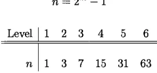
4.3

Structure

The

numberof grid

levels

m used

in

computation

is

calculated

from

n, the

sizeof

the

computational

domain

(number

of grid

points)

on

the

finest level. For

the

program

to

function

n must

be

able

to satisfy

(4.5)

where m

is

an

integer.

The

size of

the

computational

domain

on

levels 1-6 is

shown

in Table 4.1.

Level

1

is

the

coarsest

level.

n =2m

-1

(4.5)

Level

12

3

4

5

6

[image:20.533.189.345.547.620.2]

n

1

3

7

15

31

63

The

program

begins

computation on

the

coarsest

level 1

and works

up to the

finest

level

m.

Level 1

consists of

only three

grid points.

The

exact values of

these three

points are supplied.

The

two

end points are

the

Dirichlet

boundary

conditions.

The

center point

is

provided

by

the

user.

It is

assumed

that

this

point can

be

obtained

through

iterative

or

direct

methods.

Because

the

valuesofuon

level 1

[u1)

are

known

this

level is

not revisited.

The

prolongation ofu1

gives an

initial

estimate

for

u2.

One Gauss-Seidel

(GS)

iter

ation

is

then

performed on u2.

Convergence

on

the

current

level is

then

checked as

described

in

section

4.4.

If

convergence

has been

obtained on

level

2 the

program

moves

up to

level 3

(3.10).

If

not,

another

GS

iteration

is

performed on u2.

After

a

transfer

is

made

to any

level,

one

Gauss-Seidel

iteration

is

performed and

both

convergence and convergence rate are checked as

described

in

section

4.4.

If

the

convergence on

the

current

level has been

obtained

the

program moves

to

a

finer

level

(3.10).

Otherwise

if the

relaxation convergence rate

is

acceptable,

another

GS

iteration is

performed on

the

current

level. If

the

relaxation convergence rate

is

slow

the

program moves

to

a coarser

level

using

(3.8)

-

(3.9).

This

_procedure

is

_repeated until

the

convergence criteria are met on

the

finest

grid

level.

4.4

Convergence

Testing

After

each

GS

iteration,

the

norm of

the

residuals

ek

(4.6)

is

computed and con

vergence and convergence rate are

tested.

The

convergence criteria

for

the

current

operation

level is denoted

by

ek.

Convergence has been

obtained on

the

current

level

if

ek <

ek.

Finest level

convergence

em

is

provided

by

the

user.

Initial

valuesof

ek

for

all other

levels

are obtained

from

(4.7)

unless

this

calculated

ek

is

smaller

than eTO,

in

which case

ek

is

set equal

to

em.

rv^"fc ,-211/2

ek

=

[2^x

'

J

(4.6)

nk

fc

domain

nk

+

1

(4.7)

Equation

4.7

sets

ek

equal

to

the

distance between

grid points squared.

Each

time

a

transfer

is

made

to

a coarser

level

ek

is

updated:

ek

=

0.2efc+1

(4.8)

If

ek

>

fc,

convergence rate

is tested.

The

convergence rate

is

satisfactory if ek

<

rjek,

wheren=

0.5

_and

ek

holds

previous valuesof ek.

If

the

convergencerate

is

satisfactory

ek

is

set equal

to

ek

{ek

=

ek) before

another

GS

iteration

is

performed.

When

a

transfer

is

made

to

a coarser

level,

ek

is

set equal

to the

norm of

the

residuals

immediately

after

the transfer

is

made

(before

any

GS iterations

are performed).

The

value of

ek

is

not changed

immediately

after a

fine

grid

transfer

because

testing

showed

that this

decreased

program efficiency.

If

ek > r]ek

the

convergence rate

is

slow.

This indicates

that the

error

is

smooth and

should

be

approximated on a coarser grid.

4.5

Program

Outputs

After

each

Gauss Seidel

iteration,

the

errorand residuals ofeachgrid point arewritten

to

a

file.

The

error referred

to

in

this thesis

is

obtained

by

subtracting the

current

values

from

the

exact solution

(4.9).

Residuals

are calculated

from (4.10).

error =

uexact

-u

(4.9)

residuals=

Au

f

(4-10)

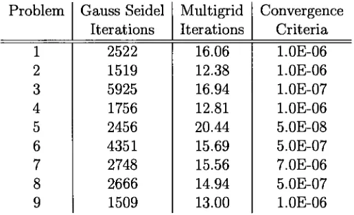
4.6

Program

Efficiency

This

program can solve equations much more

efficiently than

a solver which uses

standard

Gauss Seidel iterative

methods.

Table

4.2

shows

the

number of

iterations

required

by

the

program outlined above and a

Gauss Seidel

program

to

reach

the

indicated

convergence.

The

number of

iterations

required

for

the

multigrid program

are weighted

to

account

for

iterations

on

different

grid

levels. The

number

indicated

is the

equivalent number of

finest level

iterations.

A

single

iteration

on

level k

requires

the

same amount of work as 2~(m~fc)

iterations

on

level

m

(the

finest

level,

here level

6).

The Gauss Seidel

program

is

executed on grid

level 6

and

begins

with an

initial

guess of u =

0.

Convergence is

_{reached when}

the

_{residual norm}

(4.6)

is

less

than

or

Problem

Gauss Seidel

Multigrid

Convergence

Iterations

Iterations

Criteria

1

2522

16.06

1.0E-06

2

1519

12.38

1.0E-06

3

5925

16.94

1.0E-07

4

1756

12.81

1.0E-06

5

2456

20.44

5.0E-08

6

4351

15.69

5.0E-07

7

2748

15.56

7.0E-06

8

2666

14.94

5.0E-07

[image:23.533.142.400.283.440.2]

9

1509

13.00

1.0E-06

Chapter

5

Correction Method

5.1

Description

of

Correction

The

proposed correction

improves efficiency

by

adjusting the

values of grid points

where

large

residual spikes occur.

The

adjustments are made

immediately

after pro

longation

of

the

approximate solution when

moving to

a

finer level.

After

the

new

fine level

solution

is

obtained

the

residuals arecalculated.

The

value of

the

point at

the

location

of

the

absolute maximumresidual

is

changed.

The

new value

is

obtained

from

the

discretized

equation

(5.1),

where

Uj

is

the

point

that

is

corrected.:

1

Ui =

i-\ M

fi-^2

aiiui

~

S

aiiui

j=l J=i+1

for

i

=

\

to

M

(5.1)

Only

the

spike which corresponds

to the

maximum residual

is

corrected.

This

can

effectively increase accuracy

and requires aminimalamount of additionalwork.

This

type

of correctionworkswell when

moving to

a

fine level because

the

error

is

typically

not smooth after prolongation.

This

method

is

effective

in

reducing

error

because

residual spikes correspond

to

error

spikes.

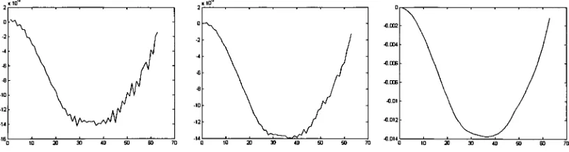
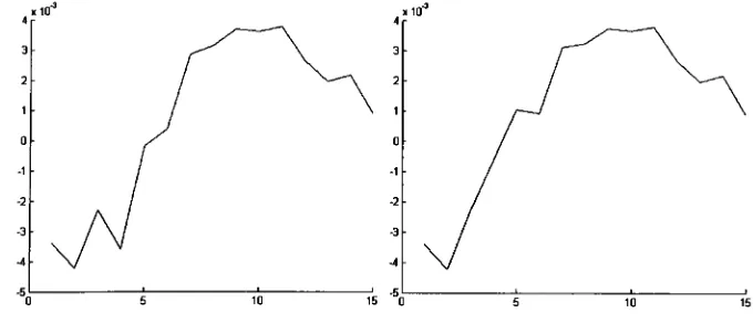
Figure 5.1

shows

the

plots of

corresponding

residual and error curves

(Problem

5,

Iteration

14).

The

largest

residual

is

at point

five,

Figure

5.2

shows

the

error plot after

this

point

has been

replaced.

The

new value of point

5 is

more accurate

than the

original.

After

one

GS iteration

the

effect of

the

correction

is

still apparent

(Figure

5.3).

When

implemented

at appropriate

times this

correction method can reduce

the

er

ror of

the

solution and reduce

the

number of

iterations

required

to

achieve residual

convergence.

The

code used

for

the

correction

is in

Appendix A. 2.

This

code was

Figure

5.1:

Problem

5,

Iteration

14.

Residual

vs.

Grid Point

(left)

and

Error

vs.

Grid Point

(right).

Figure

5.2:

Problem

5,

Iteration

14.

Error

vs.

Grid Point

after replacement of point [image:25.533.99.435.88.233.2]

5.

Figure 5.3: Error

vs.

Grid Point

one

GS iteration later

without

(left)

and with

(right)

[image:25.533.182.353.288.428.2] [image:25.533.94.434.481.627.2]

5.2

Correction

Processing

Time

The

amount of

time

required

to

perform a single correction was compared

to the

amount of

time

required

to

perform a single

Gauss Seidel

iteration.

If

residuals are

calculated

for

allgrid

points,

one correction

takes approximately the

same amountof

time to

implement

as one

Gauss Seidel iteration

on

the

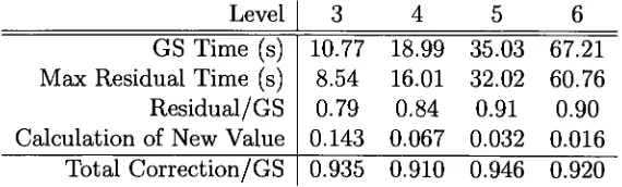
same

level. Table 5.1

shows

the

amount of work required

for

acorrectionas a

fraction

of a

Gauss Seidel

iteration.

One

correction requires

the

calculation of

residuals,

a comparison of

the

residuals

(to

determine

the

maximum

residual),

and

the

calculation of

the

new value of

the

corrected point.

Two

programs were written

to

compare

the processing time

of a

Gauss Seidel

iteration to

a

correction,

see

Appendix B. Each

program was run

four

times,

each

time

with a

different

number of grid pointvalues.

The level

number which

these

corresponded

to

is

shown

in

Table

5.1.

The

running time

required

for

each program was recorded and

is

presented

in

Table

5.1. In

the

table,

'GS

Time'

is

the running time

of

the

Gauss Seidel

program.

The

correction program

determines

the

max residual

(includes

the

calculation ofresiduals

and a comparison of

the

residuals).

This

running time

is 'Max Residual

Time'

in

Table

5.1.

'Residual/GS'

is

the

ratio of

'Max Residual

Time'

to

'GS Time'.

'New

Value

Calculation' accounts

for

the

calculation of

the

new value of

the

corrected

point.

The

amount of work required

for

the

calculation of

the

new value

is

equal

to

a

fraction

of a

Gauss Seidel

iteration,

l/nk

{nk

is

the

number of grid points on

level

k). 'Total

Correction/GS'

is the

sum of

Residual/GS

and

New Value

Calculation,

it

is

the

amount of work required

for

a correction expressed as a

fraction

of a

Gauss

Seidel

iteration.

Level

GS Time

(s)

Max Residual Time

(s)

Residual/GS

Calculation

of

New Value

Total

Correction/GS

6

10.77

18.99

35.03

67.21

8.54

16.01

32.02

60.76

0.79

0.84

0.91

0.90

0.143

0.067

0.032

0.016

0.935

0.910

0.946

0.920

Table

5.1:

Work

required

for

a correction compared

to

a

Gauss Seidel

iteration.

Table

5.1

indicates

that

a single correction requires

approximately the

same amount

of work as one

Gauss

Seidel iteration

on

the

same

level. This

means

that

acorrection

performed on

level 3

will

increase

the total

amount of work required

to

solve aproblem

by

only

0.125

equivalent

level 6 GS iterations.

Between

12

and

21

equivalent

level

6

GS iterations

were required

for

the

solution of each problem

(Table

4.2).

Thus,

a [image:26.533.125.410.440.526.2]

Chapter

6

Problems

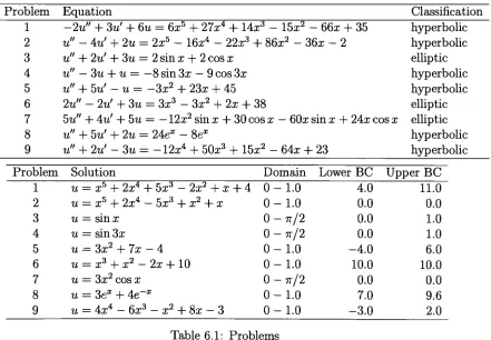
The

correction was

tested

on

the

nine problems shown

in

Table

6.1

below.

All

are

second order

differential

equations with

Dirichlet

boundary

conditions.

Problem

Equation

Classification

1

+

3m'

+

6m

= 6x5

+

27x4

+

14x3- 15x2-

-66x

+

35

hyperbolic

2

u"

- Au'

+

2u

= 2x5 - 16x4- 22,-r3

+

86x2

-36x

-2

hyperbolic

3

u"

+

2m'

+

3m

=

2

_{sin x}

+ 2

_{cosx elliptic}

4

m"

3m

+

m = _8sin

3x

9

_cos

3x

hyperbolic

5

u"

+

5'

-u =

+ 23x +

45

hyperbolic

6

2m"

-2u'

+

3m

= 3x3 - 3x2

+

2x

+

38

elliptic

7

5m"

+

4m'

+

5m

= _{sin x}

+

30

_{cos x}-

60x

sinx

+

24x

cos x elliptic

8

u"

+

hu'

+ 2u

= 2Aex - 8ex

hyperbolic

9

m"

+

2m'-

3m

=

+

50x3

+

15x2 -

64x

+

23

hyperbolic

Problem

Solution

Domain

Lower BC

Upper BC

1

u =x5

+

2x4

+

5x3 - 2x2

+

x

+ A

0-1.0

4.0

11.0

2

u = x5

+

2x4

-5x3

+

x2

+

x

0-1.0

0.0

0.0

3

u =_{sin x}

O-tt/2

0.0

1.0

4

u =_sin

3x

O-tt/2

0.0

1.0

5

m = 3x2

+

7x

-A

0-1.0

-4.0

6.0

6

u = x3

+

x2

-2x +

10

0-1.0

10.0

10.0

7

m =3x2_{cos X}

O-tt/2

0.0

0.0

8

u =3ex

+

Ae~x

0-1.0

7.0

9.6

9

u =Ax4 - 6x3 - x2

+

8x

-3

0-1.0

-3.0

2.0

Table

6.1:

Problems

The

problems were

discretized

using three

point central

differencing (6.1),

(6.2).

The

domain

ofeachproblem was split

into 64

elements of equal size

h,

yielding

acompu [image:27.533.48.489.280.586.2]

computations

(refer

to

(4.5)).

du

dx

=

^Ui+l

~ui-i)

dAu

dx2

=

Ja^Ui-x ~2ui

+

ui+i)

(6.1)

Chapter

7

Methods

To

test the

effectiveness of

the correction,

each problemwas run several

times.

These

runs are referred

to

as

trials.

The

effects of

the

correction on solution

accuracy

and

the

numberof

iterations

required

for

convergencewere measured.

The

correction was

implemented

up to three times

per

trial.

As

stated

in

Chapter

5,

corrections were made

immediately

after prolongation when

moving to

a

finer

grid

level.

In

addition corrections were

only

made after a

Gauss

Seidel

iteration

had been

performed on each

level.

The

correction

is

not effective

when applied

to the initial

iterations

in

a problem

because

the

error at each grid point

is

high. It is

most effective when

there

is

a

large

amount of

localized

error.

A

trial

was performed

for

each correction possible

based

on

the

above criteria

(indi

cated

in

yellow

in Figure 7.1).

Some

additional

test

runs with multiple corrections per run were also performed.

The

accomodative algorithm

did

not control

the

flow

of

the

correction

trials.

Instead

the

structureof

the

multigrid runswithoutcorrections

(labeled

trial

0)

was preserved

in

each of

the

correction

trials.

The

structureof

the

runs can

have

a significant

impact

on

the solution,

and

any

variance can make

it

difficult

to

evaluate

the

effects of

the

correction.

While

the

flow,

or

pattern,

of

the

runs was

preserved, the

number of

iterations

on each

level

was varied

in

accordancewith changes

in

the

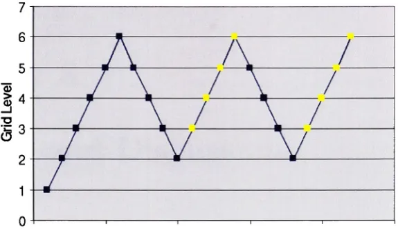
residual norm.

A

generic structure

is

shown

in Figure 7.1.

It

represents

the

basic flow

that the

accomodative algorithm used

in

this study

produced.

The

structure of each of

the

trials

performed

in this study

was a variation of

that

shown

in

Figure

7.1,

with a

varying

numberof

iterations

performed on each of

the

points

in

the

figure. Points

at

whichacorrectioncould

be

applied are colored yellow.

Plots

of

iteration

vs. grid

level

for

eachmultigrid run without corrections

(trial

0 for

each

problem)

are presented

in

Appendix C. From

the

plot of

Problem

1,

Trial 0 it

can

be

seen

that the trial

began

on

level

1,

then

moved

up

with one

Gauss Seidel iteration

performed on

levels

2,3,

and

4

and

two

GS iterations

performed on

level 5

and

level

6,

and so on.

[image:30.533.123.411.80.249.2]

Figure 7.1:

Generic

multigrid structure.

required and

the accuracy

of

the

solution.

In

Chapter 8

percent change

in

error

and percent change

in

iterations

are referred

to.

These

are

the

change

in

number of

iterations

and

the

change

in

error with respect

to the trial

without corrections

(trial

0).

%AError

=

\error\

-\errortriai0\

\errortrial0\

*100

(7.1)

^Alterations

=

iterations

iterationstriaio

iterationstriaio

*100

(7.2)

Increased

solution

accuracy

is indicated

by

a negative change

in

error.

Similarly,

a

negativechange

in iterations indicates

a

decrease

in the

number of

iterations

required

Chapter

8

Results

and

Discussion

Several

variables

influenced

the

effectiveness of

the

correction.

These included

the

nature of

the

correctederror

spike, the

grid

level

that the

correctionwas

implemented

on, the time

it

was

implemented,

and

the

grid point

that

was corrected.

Error

was

decreased in 68%

of

trials

withone correction.

The

majority

of

the

results summarized

below

areof

trials

with one correctiononly.

The

results of multiple correction

trials

are

discussed

only

in

section

8.7.

Specific

results of each

trial

are presented

in

Appendix

E.

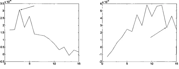
8.1

Error

Spike

Direction

The direction

of

the

errorspike

that

was corrected

had

a significant effect on whether

the

correction

increased

or

decreased

the

errorof

the

final

solution.

If

the

errorof

the

corrected point was greater

than

the

error of

the two

points adjacent

to

it,

correcting

it

generally

decreased

the

error of

the

solution

(Figure

8.1).

In

this

document,

this

is

referred

to

as a

"correct

direction"

spike

because

in the

graphical

view, the

error

spike appears

to

be

"pointing"

in

the

desirable direction.

In

some cases

the

error of

the

corrected point was negative and

the

error of

the two surrounding

points was

positive,

or vise versa.

This

situation

is

labeled

"partially

correct"

and

is

shown

in

Figure 8.2. Corrections

on

partially

correct spikes were not as effective as

those

made

on correct spikes.

In

the

caseof an

"incorrect"

direction

spike, the

error of

the

corrected point

is

smaller

than

the

errorof

the

adjacentpoints.

Correcting

an

incorrect

direction

spike

does

not always yield positive results

because

the

correction

increases

the

error of

the

corrected

point.

Figures 8.1

and

8.2

show examples of error spikes

in

the

"correct", "partially

correct" , and

"incorrect"

directions,

as

defined in

this

paper.

Overall 58%

of allspikes

were

in

the

correct

direction,

28%

in the

incorrect

direction,

and

14%

of spikes were

partially in the

correct

direction.

error

for

trials

with a single correction.

Corrections

applied

to

spikes

in the

correct

direction

produced a

decrease in

solution error

86%

of

the time.

In

the trials

in

which

corrections of correct

direction

spikes

increased

the

solution

error,

it

was

increased

an average of

only

0.8%.

Corrections

made on spikes

in

the

incorrect

and

partially

correct

directions

caused an

increase in

solution error

the majority

of

the

time.

Figure

8.1:

Error

vs.

Grid

Point,

"Correct" spike

(left)

and "Incorrect" spike

(right).

Figure

8.2:

Error

vs.

Grid

Point, "Partially

Correct" spike.

It is difficult

to

determine if

an error spike

is in

the correct,

partially

correct,

or

incorrect

direction

when

the

exact solution

is

not

known.

The

difficulty

lies

in

de

termining

whether

the

error of

the

points adjacent

to the

spike

have

a positive or

negativemargin.

The direction

of

the

spike

(pointing

up

or

down in

the

plot)

can

be

determined from

the

residuals.

If

the

diagonal

of

the

A

matrix

is

a negative

value,

the

residual spike and error spike will point

in

the

same

direction

(residual

and error

calculated

from

(4.10)

and

(4.9)).

If

the

diagonal

of

the

A

matrix

is

apositive

value,

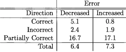
[image:32.533.95.441.176.311.2] [image:32.533.189.345.375.509.2]

Error

Direction

Decreased

Increased

Correct

Incorrect

Partially

Correct

86%

40%

44%

14%

60%

56%

[image:33.533.161.370.211.298.2]

Overall

68%

32%

Table 8.1: Percentage

of

trials

error was

decreased

or

increased

per error spike

direc

tion.

Error

Direction

Decreased

Increased

Correct

Incorrect

Partially

Correct

5.1

2.4

16.7

0.8

1.9

17.1

Total

6.4

7.3

Table 8.2:

Average

percentage change

in

error per error spike

direction.

Unfortunately,

a method of

determining

whether

the surrounding

error

has

anegative

or positive margin

has

not

been devised. Without

this

information,

knowledge

of

the

direction

of

the

spike

is

not useful.

8.2

Grid

Level

Corrections

on coarser grid

levels

proved

to

be

more effective

than

corrections on

finer

grid

levels.

Coarse level

corrections correct error on a

larger

scale

than

finer

level

corrections and

therefore

have

a greater

influence

on

the accuracy

of

the

final

solution.

This

is illustrated in

Table 8.3

and

Figure

8.6.

Table 8.3

shows

the

average

of

the

absolute value of

the

percentage change

in

final

error

for

trials

with a single

correction on

the

specified grid

level.

Figure 8.6

shows

the

change

in

error produced

by

each

trial

with a single correction and

indicates

which corrections yielded a

decreased

numberof

total

iterations. Each

data

point

is

the

result of one

trial.

The level

that

each correction was

implemented

Figure

8.3:

Error

plot

(top)

and residual plot

(bottom)

for Problem

1,

Trial

1

(level

3).

Level

3

4

5

6

Average

|

%

A Error

[image:34.533.164.370.154.322.2]

15.9

7.5

1.4

2.8

[image:34.533.190.345.507.578.2]

8.3

Point in Multigrid Cycle

The

point

in

the

multigrid cycle

that

acorrection

is

made can also effect

the accuracy

of

the

solution.

Corrections

made earlier

in

the

cycle

have

a greater

impact

on solution

accuracy than those

made

later in

the

cycle.

For

example,

if

a problem requires

36

iterations

for

convergence,

a correction made on

the

15th

iteration

will

generally

have

a greater effecton

accuracy than

a correction madeon

the

34th

iteration.

Corrections

made near

the

endof

the

cycle produced smaller errors when error

increased.

Table

8.4

and

Figure 8.5

illustrate this.

In

the table

and

figure

the

location

of

the

corrected

iteration in

the

multigrid cycle

is

given as apercentageof

the total

number

of

iterations.

Figure 8.5

shows

the

results of all of

the

single correction

trials

(in

the

same

way that

Figure 8.6 does).

One data

point shows

the

change

in

error produced

by

each

trial.

In Table

8.4 the

location

of

the

correction

in the

cycle

is

reported

in three

segments.

The

first

segment

(20-60%)

represents

the

first

set of corrections made on

any

grid

level

as

illustrated

in

Figure

8.4.

The

final

set of corrections

is

made

in

the

last

segment

(75-100%)

(Fig.

8.4).

If

three

sets of corrections were

possible, the

second

set was made

in

the

middle segment

(60-75%)

(Fig.

8.4).

Problem 5

was

the only

problem

in

which corrections were made

in

the

60-75%

range of

the

cycle

(Fig.

8.5).

7

6

5 "3

S

4

I

'

3

13

7\-ML

M-L

\

//A

,

ll\

TLL

\Li/

V

//

\

fit

F

AV^

'

~\A

v\

^jjb^j; lslset 21!et Finalset corrections

i 1

corrections

i 1

corrections

1

20 40 60 80

Location in MultigridCycle

(%)

100 120

? Correction Locations

[image:35.533.151.387.379.544.2]

Location

of

Correction In Multigrid Cycle

20-60%

60-75%

75-100%

Level

Dec. Error

Inc.

Error

Dec.

Error

Inc.

Error

Dec.

Error

Inc. Error

3

4

5

6

-15.4

43.5

-13.9

8.6

-1.2

1.1

-5.8

0.8

-0.3 -0.3

-5.6

-19.7

-11.4

11.9

-3.0

9.5

-1.3

0.6

-0.1

0.3

[image:36.533.62.474.110.229.2]

All

-9.08

13.51

-6.45 -3.95

5.57

Table 8.4:

Average

percentage change

in

error per

location

in

multigrid cycle.

60

40

20

uj

₀

<

-20

-40

-60

?

?

Level 3

Level 4

Level

5

x

Level

6

?

?

JO

2 0.00

4d!o*

X60.00

?

?

80.01*

10C

X

?

?

00

Location in Multigrid

Cycle

(%)

[image:36.533.111.431.325.606.2]

8.4

Grid Location

Corrections

on points

located

in the

center of

the

grid were more effective

than

cor

rections on points near

the

grid

boundaries.

In

the

following

discussion

grid point

locations

are expressed as a percentage of

the

computational

domain

of

the

problem.

It

should

be

noted

that

Dirichlet

boundary

conditions were used

in

all of

the

trials.

Corrections

on points

located

in the

centerof

the

grid

had

agreater

impact

on solution

accuracy than those

performed within a

distance

of

10%

(of

the

grid

length)

of

the

boundaries. Figure 8.6

shows

the

percentage change

in

solution errorvs.

the

location

of corrected point as a percentage of

the

length

of

the

grid.

The

percentage change

in

error

for

all single correction

trials

is

plotted

in

Figure

8.6.

Each

of

the

plotted points

is

the

result of one

trial.

On finer

grids errors near

the

edge of

the

grid are

reduced

by

the

boundary

conditions,

and corrections near

the

grid edges are not as

effective.

Corrections implemented

in the

center of

the

grid also

decreased

errormore

frequently

than

corrections near

the

boundary

conditions

(Table

8.5).

60.00

40.00

20.00

w

0.00

-20.00

-40.00

-60.00

-6h

20

fljFafr

t

nri-*

40"

*&

₆₀

?

80

*S*i

life

? Level 3

Level 4

A Level 5

xLevel 6

o Iterations Decreased

Grid

Location (%

span)

[image:37.533.110.434.316.611.2]

Error

of

Final Solution

Distance from

Boundary

(%

grid

length)

Decreased

Increased

0-10%

10-25%

25-50%

8

12

30

5

9

[image:38.533.97.435.82.152.2]

10

Table 8.5: Number

of

trials in

which

final

error was

increased

or

decreased

vs. cor

rection

location.

8.5

Residual Magnitude

There

was no correlation

between

the

size of

the

residual spike and

the

percentage

change

in

final

error.

Figure 8.7

shows

the

change

in

the

error of

the

solution as a

function

of

the

residual/norm

(norm

refers

to the

residual

norm)

of

the

corrected point.

8.6

Problems

The

effect of single corrections on

the

error of each problem

is

shown

in Figure

8.8.

This

plot

is

nearly

identical

to

Figure

8.6.

As in Figure

8.6,

each

data

point

is

the

result of one

trial

and

the

results of all

trials

with one correction are plotted.

In

Figure 8.8

the

problem

that

was solved

in

each

trial

is

indicated.

The

effect of

the

corrections on solution

accuracy

varied

between

problems.

Most

of

the

differences

can

largely

be

attributed

to the

factors discussed

above

(spike

direction, location,

and grid

level).

Corrections

were most effective

in

problem

5.

The

number of single correction

trials

in

which corrections were made on

correct,

incorrect,

and

partially

correct

direction

spikes

is

shown

in Figure

8.9.

In

problem

6,

100%

of

the

spikes

corresponding to the

maximum residual were

in

the

correct

direction. Problem 8

had

the

largest

number of spikes

in the

incorrect direction. The

number of

trials

performed varies

between

problems

because

of

the

variation

in

the

structureof

the

runs

(see

Appendix C). A larger

number of

trials

were performed on

problem

5 because it has

more

iterations

than any

other problem and moves

between

the

grid

levels

an additional

time.

Only

seven

trials

were performed on problem

2

because

iterations

were performed on

level 2

at

two

points

in

the

cycle

instead

of

60

50

40

w 30

20

10

?

?

?

Level 3

Level 4

A

Level 5

x

Level 6

"

?

X

?

?

%

X

V

A

A*

A

X

A X

X

X%|

->^* *

10 15

|

Residual/Norm

|

[image:39.533.112.425.193.525.2]

20 25

60.00

40.00

20.00

-20.00

-40.00

-60.00

x*

40

rj X

n*

? ₆₀ *x _{80 100}

A

Problem

Al

2

?

3

?

4

5

a6 x7 x8

o9

Grid Location (% span)

[image:40.533.116.434.214.511.2]

10

n

O

.a

E

-s

SpikeDirection

1-PartiallyCorrect

1- Incorrect

1- Correct

7 8 9

[image:41.533.65.469.224.496.2]

8.7

Multiple Corrections

The

results presented

in

the

previous sections are

the

results of

trials

with a single

correction.

Twenty-six

trials

with multiple corrections were

performed, 21

with

two

corrections,

and

5

with

three

corrections.

Appendix D

shows

the

resultsof

these trials.

The

percent change

in

error

(7.1)

and

the

percent change

in

numberof

iterations

(7.2)

are reported.

In

some cases

the

number of

iterations

did

not change and

therefore

the

percent change

in

number of

iterations

does

not show

up in the

plot.

The

graphs show

the

effects of

the

multiple correction

trials

and

the corresponding

single correction

trials

(performed

at

the

same points

in

the

cycle).

The iteration

that

a correction was

implemented

after

is indicated in

parentheses next

to the trial

number.

The iterations indicated in

the

single correction

trials

are not always

the

same as

the

iterations indicated

in the

multiple correction

trial.

This is because

some multiple correction

trials

resulted

in

a

decreased

number of

iterations

and a move

to

a

higher level

at an earlier

iteration.

The

details

of

the trials

can

be found

in

Appendix

E.

In 12

trials the

change

in

error produced

by

the

multiple correction

trial

was within

6%

of

the

sum of

the

error changes produced

by

the corresponding

single correction

trials.

Six

trials

produced an

improvement

in

solution

accuracy

over

the

combination

of

the

single corrections.

In 23

of

the

26

trials the the

change

in

number of

iterations

produced

by

the

multiple correction

trial

was equal

to the

sum of

the

changes

in

Chapter

9

Conclusions

This

study

is

an

initial

evaluation performed

to

assess

the viability

of

the

correction

method.

The

results

indicate

that

it

has

the capacity to improve

solution

accuracy

and

potentially

increase

solver

efficiency

for

a problem solvedwith multigrid methods.

The

correction can also cause a

decrease

in

solution

accuracy if

it

applied at an

improper

time.

The

most

important

factor in

determining

whether acorrection will produce positive

results

is

the

direction

of

the

corrected error spike.

Almost

all of

the

correctionsper

formed

on

"correct

direction" error spikes

increased

solution accuracy.

Unfortunately

it is

difficult

to

determine

whether or not

the

spike

is in

the

"correct"

direction. This

would

be

possible

if

a method was

devised

to

determine

whether

the

error

had

a

positiveor negative margin.

There

was also a correlation

between

the

location

of

the

correction on

the

grid and

correction effectiveness.

Error

was

decreased

in

75%

of single correction

trials in

which

the

corrected point was

in the

central portion of

the

grid.

In

most cases

implementation

of

the

correction

did

not affect

the

number of

iterations

required

for

convergence.

In

these

cases

the

amount of computational work was

increased

by