Simultaneous multithreading: Operating system perspective

Rochester Institute of Technology

RIT Scholar Works

Theses

Thesis/Dissertation Collections

2002

Simultaneous multithreading: Operating system

perspective

Vyacheslav Rubinfine

Follow this and additional works at:

http://scholarworks.rit.edu/theses

This Thesis is brought to you for free and open access by the Thesis/Dissertation Collections at RIT Scholar Works. It has been accepted for inclusion

in Theses by an authorized administrator of RIT Scholar Works. For more information, please contact

[email protected].

Recommended Citation

Simultaneous Multithreading:

Operating System Perspective

By

Vyacheslav Rubinfine

A Thesis Submitted

In

Partial Fulfillment of the

Requirements for the Degree of

MASTERS OF SCIENCE

In

Computer Engineering

Approved by:

Committee Principle:

Date:

(1-

5 -

'20

GZ GZ GZ GZ GZ GZ GZ GZ GZ GZ GZ GZ GZ GZ GZ GZ GZ GZ GZ GZ

-Dr. Muhammad Shaaban

Committee Member:

Date:

hv.cJ€

2b0

c..-Dr. Roy S. Czemikowski

Committee Member:

Date:

J,/bv-

S-:..-?

t*71.

Dr. Hans-Peter Bischof

Department of Computer Engineering

College of Engineering

THESIS RELEASE PERMISSION FORM

Rochester Institute of Technology

Simultaneous Multithreading:

Operating System Perspective

I, Vyacheslav Rubinfine, hereby grant perrmSSlOn to any individual or organization to

reproduce this thesis in whole or in part for non-commercial and non-profit purposes only.

Abstract

Developing

CPU

architecture

is

a

very

complicated,

iterative

process

that

requires

significant

time

and

money

investments.

The

motivation

for

this

work

is

to

find

ways

to

decreases

the

amount of

time

and

money

needed

for

the

development

of

hardware

architectures.

The

main problem

is

that

it is

very

difficult

to

determine

the

performance of

the

architecture,

since

it is impossible

to take

any

performance measurements untill upon

completion of

the

development

process.

Consecutively,

it is

impossible

to

improve

the

performance of

the

product or

to

predict

the

influence

of

different

partsof

the

architecture

on

the

architecture's overall performance.

Another

problem

is

that

this

type

of

development does

not allow

for

the

developed

system

to

be

reconfigured or altered

without complete re-development. .

The

solution

to the

problems mentioned above

is

the

software simulators

that

allow

researching

the

architecture

before

even

starting

to

cut

the

silicon..

Simultaneous

multithreading

(SMT)

is

amodernapproach

to

CPU

design. This

technique

increases

the

system

throughput

by decreasing

both

total

instruction

delay

and stall

times

of

the

CPU.

The

gain

in

performance of a

typical

SMT

processor

is

achieved

by

allowing

the

instructions from

several

threads to

be

fetched

by

an

operating

system

into

the

CPU

simultaneously.

In

order

to

function successfully

the

CPU

needs software support.

In

modern computer systems

the

influence

of an

operating

system on overall system

performancecan no

longer be ignored. It

is important

to

understand

that the

union of

the

CPU

and

the

supporting operating

system and

their

interdependency

determines

the

overall performance of

any

computer system.

In

the

system

that

has been

implemented

on

hardware

level

such analysis

is

impossible,

since

the

hardware

system

is

neither

flexible

nor configurable.

However,

in

the

SMT

architecture, the

system

is

capable of

performing

some useful work even

if

a

task

has

generated an error.

A

wide range of

simulators

is

described

in

the

literature,

and a

lot

of

them

are

publicly

accessible.

The

main goal of

this

work

is

to

modify

an

existing

SEVIOS/Topsy

simulator

to

process of

the

SMT

MIPS,

as well as

scheduling

aspects of

the

CPU

and

the

operating

system

integrated

environment..

This

work covers a

broad

range of

aspects,

among

which are:

1)

Completion

of

SMT

MIPS

and

SMT

Topsy

specifications;

2)

Integration

of

MXS

into

SIMOS/Topsy;

3)

Modifications

to the

fetching

unit of

MXS

that

allow

to

support

SMT;

4)

Addition

of

SMT

support

to

Topsy;;

This

work uses

Topsy/R4000

simulator

developed

at

Swiss

Federal Institute

of

Technology,

and

the

MXS

(R10000)

part of

the

SimOS

simulator

developed

at

Stanford

University.

Development

process utilizes

C

high-level

language,

Intel

and

MIPS

assembly

languages.

The

result of

this

work

is

a

development

of a complete computer system software

simulator.

The

simulator allows

taking

performance measurements andreconfigurationof

SMT

Topsy

and

the

fetching

unit of

the

SMT MXS.

The

simulator

is

modular:

that

is

any

of

its

parts can

be

substituted with otherparts

that

perform similar

functionality.

It

also means

that the

whole simulator can

be

integrated into

a

larger

scale simulation

project.

The development

of

this

simulator

significantly decreases

the

amount of

time

and

money

needed

for

the

development

of

hardware

architectures and providesnewways

in

researching

the

influence

of an

operating

system on

the

performance of

the

computer

Acknowledgements

This

work

is dedicated

to

my

family

that

has

supported and

inspired

me

during

the

difficult

time

I

have

spent at school.

I

am grateful

to

my

wife

Elena for spending

countless

hours

doing

proofreading

and other paperwork.

Thanks

go

to

my friend Slava Rozman for his

help

in

completion of successful

installation

and compilation of

the

software.

I

am grateful

to

Professor Muhammad E. Shaaban

at

the

Computer

Engineering

department

of

the

Rochester Institute

of

Technology

for raising my interest in

to

the topic

and

patiently answering

all

my

questions related

to

various computer

architectures and

operating

systems.

I

wish

to thank

him for giving

me

the

opportunity

to

work on

this

project and

shaping my

learning

with

his

valuable

Trademarks

This

work

is

based

on

the

following

software:

SimOS

Trademark

of

Stanford

University

Table

of

Contents

List

of

Figures

3

List

of

Tables

5

Glossary

of

Terms

6

Chapter 1. Introduction

8

1.1. Basic

architectures and

techniques

8

1.2. Pipeline

and

hazards

10

1.3.

Superscalar

architecture and

SMT

15

1.4. Overview

ofsubsequentchapters

16

Chapter 2.

Developing

SMT

SimOS/Topsy

environment

17

2.1. Basic

SimOS/Topsy

environment

17

2.2.

Switching

to

SMT

SimOS/Topsy

environment

18

2.2.1. Problems

associatedwith

basic

SimOS/Topsy

environment

19

2.2.2. SMT

SimOS/Topsy

environment

19

2.2.3.

Work

cycle of

the

SMT

SimOS/Topsy

environment

21

2.3. Annotations

vs.

Performance Counters

23

Chapter 3.

Developing

SMT MXS CPU

model

26

3.1. General

Description

27

3.2.

Instruction

Set

29

3.3.

Pipeline

34

3.4.

Caches

38

3.4.1.

Primary

Instruction Cache

38

3.4.2.

Primary

Data

Cache

38

3.4.3.

Secondary

Cache

39

3.4.4.

Cache

Algorithms

39

3.4.5.

Virtual

Address

Translation

and

Pages

40

3.5.

Fetching

Unit

of

SMT

MXS CPU

model

41

3.5.1

Basic

MXS

Fetching

Unit

41

3.5.2

SMT

MXS

Fetching

Unit

42

3.5.3

Enhanced

SMT

MXS

Fetching

Unit

43

3.6. Register

Renaming

Unit

and

Special

Techniques

47

3.6.1.

Operating

System

Support

for

Register

Renaming

49

3.6.2.

Compiler

Support for

Register

Renaming

51

3.6.3. SMT

MXS Support

for

Register

Renaming

53

3.7.

SMT

Issue

Queues

55

3.7.1

Integer

Queue

55

3.7.2 Floating-point

Queue

56

3.7.3. Address

Queue

56

3.8.

Branch Prediction Policies

57

3.9.

Branch Prediction

Unit

of

SMT

SimOS

65

3.10. WRITE

Branch Prediction

Policy

72

3.11.

Exception

Handling

in

SMT

MXS

72

3.1 1.1.

Cold

Reset Exception

74

3.11.2.

Soft

Reset Exception

75

3.11.4.

TLB

Exception

76

3.11.5. System Call Exception

78

3.12. SMT MXS Coprocessor 0

79

Chapter 4.

Developing

SMT

Topsy

83

4.1. Slow Interrupts

83

4.2. OS:

loading

executable

files

88

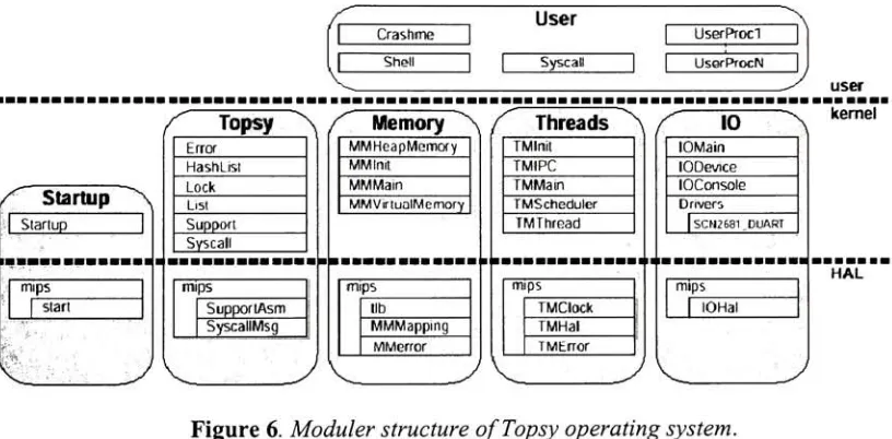
4.3. Topsy:

current architecture

89

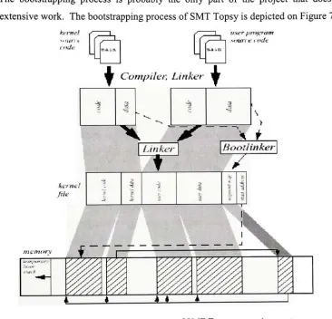
4.4.

Switching

to

SMT:

Bootstrapping

process

90

4.5. SMT startup

and

dynamic

loading

92

4.6. SMT Threads Module

93

4.7. Demand

Paging

in SMT

Topsy

101

4.8.

SMT

Memory

Management Module

103

4.9.

SMT Scheduler

106

4.9.1. Basic

Topsy

Scheduler

106

4.9.2. SMT

Topsy

Schedule

107

4.9.3. SMT

Topsy

Scheduler Interface

1

10

4.10.

Exception

Handling

1 1 1

4.11. SMT

Topsy

Shell

112

Chapter

5.

Simulation

Results

1 14

5.1.

SMT

fetching

unit performance

114

5.2.

SMT

Topsy

schedulerperformance

119

Chapter

6.

SMT MXS

SimOS/Topsy

Installation

and

Configuration

124

6.1.

Binary

Utilities

installation instructions

124

6.2.

MIPS

Cross-compiler installation instructions

125

6.3.

SMT

SimOS/Topsy

integrated

environment

installation instructions

125

6.4. SMT

MXS

SimOS/Topsy

Configuration

127

Chapter

7.

Conclusion

130

List

of

Figures

Figure 1. Basic

SimOS/Topsy

environment.

Page

17.

Figure 2. SMT

SimOS/Topsy

environment.

Page

19.

Figure

3.

Work

cycle

of

SMT

SimOS/Topsy

environment.

Page 21.

Figure

4.

Viewing

data

with

RIT

Viewer

application.

Page 24.

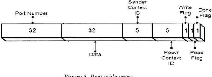
Figure 5.

Port

table

entry.

Courtesy

of

Dominik

Madoh,

Eduardo

Sanchez,

Stefan

Monnier,

Computer Science

Department,

Yale

University.

Page 32.

Figure 6.

Modular

structure

of

Topsy

operating

system.

Courtesy

of

George

Fankhauser,

Christian

Conrad,

Eckart

Zitzler,

Bernhard

Partner,

Computer

Engineering

and

Networks

Laboratory,

ETH Zurich. Page

89.

Figure

7.

Bootstrapping

process

of SMT

Topsy

operating

system.

Courtesy

of

George

Fankhauser,

Christian

Conrad,

Eckart

Zitzler,

Bernhard

Partner,

Computer

Engineering

and

Networks

Laboratory,

ETH Zurich. Page 90.

Figure 8. Kernel

thread

messages queue organization

of

Topsy

operating

system.

Courtesy

of

George

Fankhauser,

Christian

Conrad,

Eckart

Zitzler,

Bernhard

Partner,

Computer

Engineering

and

Networks

Laboratory,

ETH Zurich.

Page 97.

Figure

9. Kernel

threadmessages queue organization

ofSMT

Topsy

operating

system.

Page 98.

Figure

10.

SMT MXS

fetching

process.

Page 106.

Figure 12. BasicMXS

Fetching

Unit

performance.

Page 114.

Figure 13. SMT MXS

Fetching

Unit

performance:

2

contexts.

Page 115.

Figure 14. SMT MXS

Fetching

Unit

performance:

4

contexts.

Page 116.

Figure 15. SMT

MXS

Fetching

Unit

performance:

8

contexts.

Page 1

17.

Figure 16.

Comparing

none-SMTand

SMT

MXS

Fetching

Units. Page 117.

Figure

17.

Comparing

none-SMTand

SMT

MXS

Fetching

Units. Page 118.

Figure

18.

Basic

Topsy

scheduler.

Page

118.

Figure 19. SMT

Topsy

scheduler.

Page 1 19.

Figure 20. Basic

Topsy

scheduling

process.

Page 120.

Figure 21.

SMT

Topsy

scheduling

process.

Page

121.

Figure

22.

SMT

Topsy

scheduling

process.

Page 122.

Figure

23.

Comparing

SMT

Topsy

scheduling

processes,

List

of

Tables

Table 1.

Main

configuration parameters

ofSMT

SimOS/Topsy

environment.

Page 20.

Table

2.

Viewing

data

with

RIT

Viewer

application.

Page

24.

Table 3. General

specification

of

SMT

microprocessor.

Page

28.

Table

4. Instructions

compatibility in SMT

microprocessor.

Page 37.

Table 5.

Operational

modes

ofSMT

MIPS

microprocessor.

Page

40.

Table

6. SMT Coprocessor 0

instructions.

Page 79.

Table 7. Number

and

types

of

registers

in SMT MXS

CPU

model.

Page

127.

Table

8. Parameters

related

to

register

renaming

and

load/store

operations

in SMT MXS

simulator.

Page

128.

Table 9. Bandwidth

parameters

of SMT MXS

simulator.

Page 128.

Table

10.

Branch

prediction parameters

ofSMT MXS

simulator.

Page 129.

Table

11.

Latencies of

the

various operations

of

thefunctional

Glossary

of

Terms

Superscalar

-

CPU

architecture

that

can

fetch,

execute and complete more

that

one

instruction in

parallel.

ANDES

-

Architecture

with

Non-sequential Dynamic

Execution

Scheduling

Dynamic instruction scheduling

-

CPU issues

an

instruction

as soon as all

its

operands

become

availableand

the

required execution unit

is

not

busy.

Out-of-order

execution

-in Superscalar CPU -instructions

can

be

executed not

in

program order..

Speculative

branching

-the

CPU

executes

the

branch

based

on

the

previous

history

of

the

branch

or

based

on

its

own

fetching

policy,

since

there

is

not enough

time

for

the

CPU

to

calculate

the

real

branch

address

due

to the

CPU fetch bandwidth.

Non-blocking

cache

-type

of

cache,

in

which cache misses

do

not stall

the

CPU.

Wrong-path instructions

-

instructions

that

were

fetched

as

the

result of

branch

misprediction.

Pipeline

-the

process of

dividing

of each

instruction into

a sequence of simpler

suboperations

(stages),

each of which

is

performed

by

a separate

hardware

unit.

Pipeline

latency

-

the

number of cycles

between

the time

an

instruction

is issued

and

the time

the

dependent

instruction

(the instruction

which uses

its

resultas an

operand)

can

be issued.

Precise

exception

handling

-

technique that

_allows

handling

of an exception at

the

moment

it

occurs.

A

typical

processor

design implements

precise exceptions

by:

1)

identifying

the

instruction,

which caused

the exception;

2)

preventing

the

exception-causing instruction

from

graduating;

3)

aborting

all subsequent

instructions.

Strong

ordering

-

in-order

instruction

_graduation

maintained, though the

instructions

may

be issued

and executed out-of-order.

Register renaming

-

logical

_registers specified

in

the

operands are mapped

to

Forwarding

logic

-

hardware

that

makes

the

result of an

instruction

available

for

subsequent

instructions before

the

instruction

graduates.

Dead-register distance

-the

number ofcycles passed

between

a register's

last

use and

its

redefinition.

HAL

-hardware

abstraction

layer.

SMT

-simultaneous multithreading.

The

SMT-capable

CPU

can process

instructions from

several processes simultaneously.

The SMT-capable operating

system can

have

several processes

in running

state simultaneously.

SIMOS

-complete machine simulator environment

developed

at

Stanford

University.

SMT

SIMOS

-completemachine simulator environment

that

supports

SMT.

Topsy

-simple

Teachable

Operating

System

developed

at

Swiss

Federal Institute

of

Technology.

SMT

Topsy

-Topsy

that

supports

SMT.

MIPS

-

CPU

type.

Can be

referred

to

in

conjuntion with

R3000, R4000, R10000,

or

R12000

processors.

SMT MIPS

-

MIPS

processor model

that

supports

SMT.

SIMOS/Topsy

-

integrated

environment

that

includes

both

SEVIOS

and

TOPSY.

SMT

SIMOS/Topsy

-SIMOS/Topsy

that

supports

SMT.

MXS

-part of

SEVIOS

that

implements

R10000

CPU.

SMT MXS

-

MXS

that

Chapter

1.

Introduction

Section

1.1

illustrates

basic

architectures and

techniques that

are used

in CPU

design.

Section 1.2 describes

the

issues

related

to

pipelining

and problems associated with

this

technique.

Section 1.3

represents superscalarand

SMT CPU

architectures.

Section 1.4

providesan overview of

the

subsequent chapters.

7. 7.

Basic

architectures and

techniques

During

the

second

half

of

last

century

computer

technology

has

made

incredible

progress.

The

microprocessorperformance growth

improved

at

the

rateof

roughly

35%

per year

[1].

Any

modern computer architecture

has

to

satisfy

various

requirements,

such as:

1)

Instruction

set architecture should refer

to

the

actual visible user set of

assembly

instructions.

At

the

same

token, it has

to

be

minimal,

yet

flexible

enough, to

allow

the

user

to

manipulate all aspects of

the

contemporary

CPU.

2)

Modern memory

hierarchy

should not

only

include

physical

implementation

of all

the

levels

of

caches,

but

alsoeffective

memory

management strategies.

These

strategies

imply,

but

not

limited

to

increasing

the

hit/miss

cache

ratio,

memory consistency

and access and

managing

persistentmedia.

3)

Performance

should

include

such aspects as

instructions

scheduling

and

execution;

hardware

interrupts.

4) Operating

systems specifics should

include

processes

scheduling,

process

memory

management,

software

interrupts,

file

systems andother aspects.

In

light

of

the

complicated

tasks

mentioned

above, and,

in

particular,

of

the

CPU

performance

requirements, this

work addresses

the

following

issues:

1)

General definition

of

the

main principals of

high

performance

CPUs.

2)

Formulation

of

the

hardware

and software requirements

for

the

CPU

model

along

with

3)

Determination

of

the

factors

that

allow most efficient

interaction between

a

UNIX-type

operating

systemand

the

high

performance

CPU.

4)

Identification

and

implementation

of a set ofchanges

to the

operating

system

that

allows reliable use of

SMT

features.

5)

Foundation

for future

research and

development in

the

area of computer

engineering

consistent with

the

findings

presented

in

this

work.

The

formula

presented

below is

used

to

calculateperformance of

any

CPU:

P

=

IC

*

CPI

*

T;

Where: IC

-instruction

counter,

indicates

the total

numberof

instructions in

a

program;

CPI

-cycles per

instruction,

indicates

the

number of machine

(command)

cycles per

instruction;

T

-clock cycle

time that

is

individually

measured

for

each

type

of

CPU.

This formula determines

that

the

CPU

execution

time

is

equally

dependent

on all ofthe

three

parameters:

IC,

CPI

and

T.

Since

T

is

a constant

hardware

characteristic of eachparticular

type

of

CPU

and

does

not change

depending

on process parameters and

organization, this

work

is

mostly

dedicated

to the

other

two

component of

the

equation:

IC

and

CPI.

The

stack-based

CPU

designs

suggested a good

IC

*

CPI

ratio

by

allowing

all operations

to

utilize

the

stack.

In

that case, the

CPU

was

waiting

on

the

first

operand

to

be

pushed onto

the stack, then

for

the

second operand

to

be

entered

likewise,

the

operation

to

occupy

the

top

of

the stack, and,

at

last,

for

execution

to take

place.

The

accumulator-based architectures employed

slightly

different

approach.

One

operand was

loaded into

a special purpose

register,

also called

accumulator,

and

the

other operand was accessed

directly

from

memory

or

loaded into

another

temporary

location

and accessed

from

there.

Those

two

instruction

set architectureswere named register-register and

register-memory

architectures accordingly.

They

both

presented

advantages,

as well as

disadvantages:

disadvantage

of

the

register-register architecture

is

that

instructions

cannot

directly

refer

to

memory;

the

IC

for

this

architecture

is higher

than

for

the

register-memory

architecture.

2)

The

advantage of

the

register-memory

architecture presents good code

density,

which

yields

the

good

IC.

Because

the

instructions

contain

direct memory

references,

data

can

be

accessedwithout

loading

first. One

of

the

disadvantages

of

the

register-memory

architecture

is

that

even

though the

CPI

parameter

for

this

architecture

is lower

than

for

the

register-register

architecture,

the

operandsare not equal

in

size.

Another

disadvantage

of

the

register-memory

architecture

is

that

encoding

a register number and a

memory

address

in

each

instruction

may

restrict

the

number ofregisters.

The

listed

above architectures presented a significant

freedom

to

computer engineers

and

designers.

However,

neither of

the

architectures could produce a significant

boost in

the

CPU

performance.

The

reason

for

that

was

that the

CPU

executed all

the

instructions (no

matter

from

where

they

were

taken)

sequentially.

Therefore,

the total

execution

time

depended

linearly

on

the

number of

the

instructions introduced

by

a particular process.

On

the

other

hand,

analysis of processes showed

that

a

typical

process

had

a

large

number of independent

instructions. The CPU designers faced

a great challenge

in

developing

technique

that

allows multiple

instructions

to

be

simultaneously

issued

to the

CPU.

1.2. Pipeline

and

hazards

The

basic idea

of

pipelining

(the

new and

promising

way

of

issuing

multiple

instructions

to

the

CPU)

is

simple: similar

to

an

assembly

line,

an

instruction

execution

is

broken

up

into

several steps.

Different

stages complete particular parts of various

instructions in

parallel.

Each

of

these

steps

is

named either a pipe stage or a pipe segment.

This instruction

execution

time

can

be

calculated as a product of

the

number of pipeline

stages

(the

pipeline

depth)

and

the

length

of

the

slowest pipeline

stage,

assuming

that there

are no problems

during

the

execution

that

may

postpone

the

execution of

the

instruction.

Such

time

is

required

to

measure

the

ideal

performanceof

the

pipeline.

In

real

life, however,

the

execution

time

of an

instruction in

the

pipeline

is significantly different from its ideal

due

to

a number of

factors.

These

factors

are called

hazards

and categorized

into

several

groups,

depending

on

their

nature.

The

following

paragraphs provide more

details

on

the

pipeline

hazards.

Any

hazard

prevents

the

next

instruction in

the

instruction

stream

from

executing

during

its designated

clock cycle.

There

are

three

classesofhazards [1]:

1)

structural

hazards

that

arose

from

resource conflicts when

the

hardware

could not provide so called

"support

orthogonality".

In

other words structural

hazards

occurred when not all possible combinations of

instruction

could

be

supported

by

the

hardware.

2)

data hazards

that

arose when

the

instruction depends

on

the

results of

the

previous

instruction in

a

way

that

was exposed

by

overlapping

of

instructions in

the

pipeline.

3)

control

hazards

caused

by

branches

and other

instructions

that

changed

the

PC.

The

following

is

a more

detailed discussion

on

the

structural

hazards.

The

most common

instances

of structural

hazards

occurred whensome

functional

units

were not

fully

pipelined.

In

technical terms

it

meant

that

a particular

functional

unit or

the

number of

functional

units could not execute

the

instructions

at

the

rate of one per clock cycle.

According

to

[1],

when

the

sequence of

instructions

encountered

this

hazard,

the

pipeline stalled one of

the

instructions

until

the

required unit

became

available.

Some

pipelines contained mixed

instruction

and

data

streams,

whichincreased

the

average number of pipeline stalls.

As

the result, the

majority

of modem machines

have

separate

instruction

and

data

pipelines.

Another

solution

in

preventing

structural

hazards is

the

duplication

of

hardware

units.

For

more

details

on structural

hazards

please refer

to

[1].

The

next and more serious

type

of

hazards

is

the

data hazard.

There

are

many

situations when a particular

instruction

got a

wrong

operandas

the

result of non-finished execution of

its

predecessor,

or an operation not

being

overwritten

before

the

instruction

waiting

for

this

result

had

a chance

to

read

it. Data hazards

can

be described

as one of

the three

types,

depending

on

the order,

in

which read and write accesses occurres

in

the

instructions.

For

two

instructions

A

and

B,

with

A occurring before

B,

the

possible

data hazards

are:

1)

RAW

(read

after

write)

-

B

attempted

to

read a source

before

A

wrote

it,

2)

WAW

(write

after

write)

-B

tried to

write an operand

before it

was written

by

A,

and

3)

WAR

(write

after

read)

-B

proceeded with

techniques

will

be

mentioned

further down

as a part of

presenting

instruction-level

parallelism

in

pipelining.

As

it is

shown

in

[1],

the

data hazards

caused a great

deal

of performance

loss in

the

pipeline.

However,

control

hazards

are always considered

to

be

the

main sourceof

the

loss

of

the

CPU

performance.

The

simplest

way

to

deal

with

the

control

hazards is

to

stall

the

pipeline as soon as

the

hazard

was

detected. In

other

words,

the

pipeline

had

to

be

stalled untill

the

new value of

PC

wascalculated.

However,

in

order

to

really

solve

the

problem,

the

CPU designers had

to

find

answers

to the

following

questions:

1)

how

to

determine

whether

the

branch

was

taken

or not

taken

earlier

in

the

pipeline and

2)

how

to

compute

the taken

PC

(i.e.,

the

address of

the

branch

target)

earlier.

The

length

of

the

control

hazard

was called a

branch delay.

In

general,

the

deeper

pipeline,

the

worse

the

branch

penalty

was

in

clock cycles.

Here

several choices of

reducing

pipeline

branch delays

will

be

considered.

As

it

was presented

above,

the

simplest scheme

to

handle branches is

to

stall

the

pipeline.

A

higher

performance,

but

somewhat more

complex,

scheme was

to

predict

the

branch

as not

taken,

simply

allowing

the

pipeline

to

proceed as

if

the

branch

were never

executed.

An

alternative scheme

is

to

predict

the

branch

as

taken

and always continue

the

execution at

the

branch

target

instruction

address.

Yet

another scheme was

developed

that

was called

delayed branch.

This

scheme placed

the

sequential successors of

the

branch in

the

branch-delay

slots.

These instructions

were executed whether or not

the

branch

was

taken.

The

modem and

the

most practical use of

this

scheme

is

that

branches have

a single

instruction

delay

slot.

There

were

many

other

techniques the

computer engineers

introduced

to

prevent control

hazards.

For

more

details

on prevention of control

hazards

please refer

to

The

listed

above explained

how

pipelining

could

overlap

the

execution of

instructions

when

the

instruction

were

independent

ofone another.

Several

techniques

were

introduced

to

extend

the

pipelining

ideas

by increasing

the

amount of parallelism

introduced

by

many

instructions.

Consider

the

case with

three

instructions

A, B,

C

where

the

instruction C did

not

depend

on either

A

or

B,

than the

execution of

C

was postponed until

it

commits

the

results

presenceofstructural and

data

hazards,

the

instruction had

to

wait

for its

operands

to

become

ready.

Only

after

both

operands

had been

present was

the

instruction ready

to

move

to the

execution stage.

It clearly

showed

that

in

somecases an

instruction had

to

occupy CPU

units

for

significant

time;

the

whole pipeline

had

to

be

stalled while some

instructions

were

actually

able

to

execute.

The logical

solution

to this

problem was

to

split

the

decode

stage

into

two:

issue

and read operands stages.

If

there

were no structural

hazards,

the

instruction

would

be

checked against

the

readiness of

its

operands,

and

if

any

operand were not

ready

due

to the

data

hazard,

the

instruction

would not

be issued

to

an appropriate

CPU

unit,

but

into

the

queue.

Moreover,

since

the

execution phase might span a

few CPU

cycles, the

CPU

designers distinguished between begin

and complete execution phases.

The

technique

of

introducing

multiple

instructions

to

CPU

execution units was named

"dynamic

scheduling" and

became extremely

popular

in

a

very

short

time.

The

following

subsections

briefly

describe different

techniques

for dynamic

scheduling,

their

advantages and

disadvantages,

as well as

inability

to

solve certain problems

that

arose

for

the

computer engineers at

that time.

Scoreboarding [1]

was used

in

those

cases when

the

CPU

executes

instructions in

an out-of-order manner

in

the

presence of sufficient

hardware

resources and absence of

data

hazards.

As

described in

[1],

every instruction

went

through the scoreboard,

wherea record of all

data dependencies

was constructed.

This

action

implied

WAW

hazard

checking,

as well as

the

availability

of

the

appropriate

functional

units.

Only

if

no other

instruction

wanted

to

write

the

result

to the

output

register,

and

the

unit was

free,

was

the

instruction

issued.

Then

the

scoreboard

determined

when

the

instruction

could read

its

operands and

begin

execution.

The instruction

was

executed,

and

the

scoreboard was notified upon

its

completion.

If

no

WAR

hazards

were

detected,

the

scoreboard

then

wrote

the

result

in

memory

[1].

The

disadvantages

of

scoreboarding

were:

1)

scoreboarding did

not allow

forwarding,

since

it

could

only apply

operands after

both

of

them

had been

placed

into its

registers;

2)

scoreboarding

was

getting

all

the

information from

communication with

functional

units,

which was

limited

by

the

number of available operands/result

buses in

a register

file.

Perhaps,

the

most significant

limitations

of

scoreboarding,

according

to

[1],

were

the

that

could

be

found),

and

the

number of scoreboard entries

(scoreboard

window,

i.e.

the

number of

instructions

that

could

be actually

placed

for

execution at

any

time).

Because

dynamically

scheduled pipeline

introduced

more

data

dependencies,

another

technique,

known

asregister

renaming,

or

the

Tomasulo

Approach,

was

introduced.

Tomasulo Approach

was used

primarily in

those architectures;

where

the

number of

functional

units was not

significant,

though the

units

themselves

were pipelined.

Instead

of compiler register

renaming,

the

WAW

/

WAR

dependencies

elimination was achieved

by

use ofreservation stations.

The

reservation stations

buffered

the

operands of

instructions

that

were

waiting

to

be issued

by

the

issuing

logic [1].

First,

the

reservation station saved

the

operand

eliminating

the

need

to

get

it from

the

register.

Second,

any

pending

instructions

could use reservations stations as

their

input.

Finally,

the

WAW

hazards

could not

happen

due

to the

fact

that

only

the

last

write operation

to the

reservation station

actually

caused

the

register update.

As

specified

by

[1],

there

were

two

significant advantages

in

the

organization of

Tomasulo's

schema:

1)

hazards detection

and execution control were

distributed,

since

the

reservation station at

every

functional

unit

decided

when an appropriate

instruction

could execute at

the unit;

2)

the

results were passed

from

the

reservation stations

directly,

eliminating

the

need of use of registers and associated

data

hazards.

As

the

result of all

the

aspects mentioned

above, the

Tomasulo's

technique

was usefulon single-issue pipelines with

limited

number ofregisters.

Even

though

a number of other

techniques

were also

developed

to

improve CPU

performance,

none of

them

could

increase

the

numberof executed

instructions

per cycle

to

1.3. Superscalar

architecture

and

SMT

Consistent

with

the

definition

of a

base

scalar processor

[2],

simple operation and

instruction latencies

were all equal

to

one,

the

Superscalar

processor

issued

multiple

instructions

and generated multiple results per cycle.

A

vector processor executed vector

instructions

on

the

arrays of

data

such

that

each

instruction invoked

a

string

of parallel

operations.

This

was

ideal for

pipelined architecture with one result per cycle.

In

theory,

according

to

[3],

a

Superscalar

processor

may

reach

the

same performance as a machine with vector

hardware.

If

a

Superscalar

machinecould

issue

a

fixed-point,

floating-point,

load

and

branch,

all

in

one

cycle,

the

effect would

be

the

same as

from

the

use of vector

load

chained with vector add machine.

A

typical

VLIW

(very long

instruction

word)

[2]

machine

had

instruction

words

hundreds

of

bits in length.

Like

in

a

Superscalar

processor,

multiple

functional

units were used concurrently.

All

unitsshared

the

common register

file.

The

concept of micro

coding,

as stated

by

[2],

implied

the

use of

different

fields

of

the

long

instruction

word

to

carry

the

operation codes

in

the

order

to

be dispatched

to

different

functional

units.

Indeed,

the

code written

in

conventional short

instructions had

to

be

combined

to

use

in

VLIW

computers.

However,

the

vector machines are

beyond

the

scope of

this

work,

and

for

this reason, this

work will

focus

on

Superscalar

architecture only.

The

issue

utilization

in

the

superscalar

architecture,

i.e.

the

percentage of

issue

slots

that

were

filled

each

cycle, along

with

the

cause

for

every empty

slot was measured

using

the

SPEC benchmark.

If

the

next

instruction

could not

be

assigned

during

the

same cycle as

the

current

instruction,

then

the

remaining

issue

slots at

this

cycle,

as well as

issue

slots of

idle

cycles

during

the

execution of

the

current

instruction,

were assigned

to the

causes of

the

delay.

In

case of overlapped

causes, the

longest

delay

wasassigned.

The

results showed

that

the

functional

unitswere

highly

underutilized.

On

average,

according

to

[2],

the

architecture reached

only

1

.5

instructions

per

cycle,

witha

full

8-way

issuing

schema.

Also,

it

was clear

that there

was no

any dominant

source of wasted

issue bandwidth.

Although

there

were

dominant items in

individual benchmarked

applications, the

dominant

cause was

different in

each case.

All

above

listed

major

techniques

of

reducing

the

waste were applied.

None

of

them,

though,

produced a

satisfactory increase

in

performance,

since

they

only

attacked

was notcapable ofcomplete elimination ofeithervertical waste

(completely

idle

cycles)

or

horizontal

waste

(unused issue

slots

in

a non-idle cycle).

1.4. Overview

of subsequent chapters

Chapter

2,

Developing SimOS/Topsy

Environment,

provides

basic

information

about

the

initial integrated

model

for

the

development.

The

chapter

describes necessary

modifications

to

convert

the

initial

integrated

environment

to

the

SMT MXS

integrated

environment.

Chapter

3,

Developing

SMT

CPU Model

introduces

theoretical

foundation

and a set

of requirements

for SMT CPU.

The

chapter

includes

several

implementation

issues,

along

with

the

results of

instruction

fetching by

the

SMT MXS

fetching

unit.

Chapter

4,

Developing

SMT

Topsy

describes

a set of changes

to the

modern

operating

system

(Topsy)

to

accommodate

the

SMT

scheduling.

This

chapter also provides particular

implementation

details

of

the

SMT MXS

scheduler.

Chapter

5,

SMT

MXS

SimOS/Topsy

Installation,

describes

the

process of

installation

of

the

SMT

MXS

SimOS/Topsy

integrated

environment on a user's

PC (Linux

platform).

Chapter

6,

SMT

MXS

SimOS/Topsy

Configuration,

describes

the

process of

Chapter 2.

Developing

SMT

SimOS/Topsy

environment

Section 2. 1 discusses

the

basic

SimOS/Topsy

integrated

environment and

its

work

cycle.

Section 2.2

introduces

a

few

problemsassociatedwith

the

basic

environment.

Section 2.3 illustrates

advantagesof

the

SMT

SimOS/Topsy

and

describes its

working

cycle.

Section 2.4 demonstrates

a new

Performance Counters

concept

that

is

used

to

monitor

the

work cycle of

the

SMT

SimOS/Topsy

integrated

environment.

2.1.

Basic

SimOSITopsy

environment

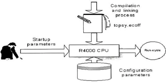
This

section provides an overview of

the

basic integrated

environment,

which

structure

is

shown

in Figure

1

.

*

Startup

parameters

^J

Compilation

^jj^-and _linking

K

s

process ,1 topsy.ecoff

R4000 CPU

[image:24.527.123.403.392.531.2]

Configuration parameters

Figure I.Basic

SimOS/Topsy

environment

In

order

to

be

executed

by

the

SimOS

simulator,

Topsy

has

to

be

compiled and

linked

using

MIPS

cross-compiler.

The

output

file,

topsy.ecoff, is

then

loaded

into

the

SimOS

secondary

caches,

as well as

the

implementation

of

the

virtual machines and

CPU

vectorization,

are

disabled.

2.2.

Switching

to

SMT

SimOSITopsy

environment

As

indicated in

[3],

SMT is

a

latency-tolerant CPU

architecture

that

is

able

to

execute

multiple

instructions

from

multiple

threads

during

each cycle.

This

ability

to

issue

instructions from different

threads

provides

for

a

better

utilization ofexecutionresources

by

converting

thread-level

parallelism

into instruction-level

parallelism.

A

number of previous

studies

have

established

that

SMT

is

an effective

instrument for

increasing

performance ona

variety

of

workloads, and,

at

the

same

time, it

provides good performance

for

single-threaded

applications.

As

it

was shown

in

[1],

at

the

hardware

level,

SMT usually

serves as an extension

to

any

out-of-order superscalar.

A

good example of

this

would

be

the

fact

that the

SimOS

uses

Alpha

21264

as

the

bases

for

SMT

features

implementation.

However,

the

Alpha

architecture, though

very

wellsuited

to

work on

any IRLX/MIPS

based

system,

is

not

easy

to

acquire andaccommodate.

For

this

reason

implementation

of

SMT

on

the

MIPS R10000

has

been

chosen.

In

addition

to the

difficulties

with

Alpha 21264

mentioned

above, the

decision

to

implement

SMT

on

the

MIPS R10000

was

based

uponother

reasons,

such as:

1)

Comparably

large

selection of

documentation

materials available

for

R10000;

2)

Compatibility

of

Rl

0000

with

Topsy;

3)

A

discovery

ofa

very

well-structured

R4000/Topsy

simulator

(see

previous

section);

Even considering

all

the

advances of

SMT,

there

are still some

improvements

to the

underlying hardware

needed

to

be

added

in

order

for

SMT

to

be implemented

on a single

CPU

architecture.

These improvements

wereas

follows:

1)

Duplication

of

the

register

file,

program

counter,

subroutine stack and

internal

processor registers of a superscalar so

that the

state of multiple

threads

(contexts)

can

be

held;

2)

Implementation

of

the

per-context mechanisms

for

pipeline

flushing,

instruction

2.2.1. Problems

associated

with

basic

SimOS/Topsy

environment

There is

the

number of problems

that

need

to

be

resolved

in

order

to

switch

from

the

basic

SimOS/Topsy

environment

to the

SMT

SimOS/Topsy

environment:

1)

Initial MXS CPU

model

is in

non-working

state

2)

The MXS CPU

model

is

not

integrated

into

the

basic

SimOS/Topsy

environment

3)

The basic

SimOS/Topsy

environment

does

not provide

full

support

for instruction

and

data

caches:

the

instruction

and

data

caches cannot

be

loaded

with

the

appropriate segmentsof

Topsy

kernel

4)

The

Topsy

kernel

requires

installation

of

binary

utilitiesand

MIPS

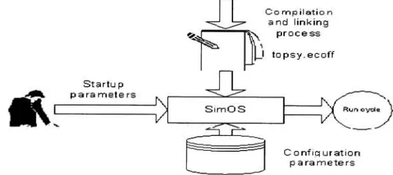
cross-compiler

2.2.2. SMT

SimOS/Topsy

environment

Figure

2

shows

the

modified

SimOS/Topsy

integrated

environment.

~L

Cornp ilation and

linking

ijv process

^

Startup

parameters

Configuration pa ra meters

Figure

2. SMT

SimOS/Topsy

environment

Upon

completion of

the

compilation and

linking

processes,

the

output

file,

topsy.ecoff,

is

placed

in

the

root

SimOS

directory.

The

modified

SimOS

simulator

includes

the

implementation

of

primary

and

secondary

caches and

the

implementation

of

the

vector of

virtual machines.

Each

of

the

virtual machines can read

instructions

and

data from

instruction

and

data

caches.

Both

the

instructions

and

data

can

then

be loaded into

the

vector

of

CPUs (maximum

number of

CPUs

associated with each machine

is

32)

and executed

by

each of

the

CPUs. Both

cache and

CPU

modelsare configurable.

Even

though there

are

few

[image:26.527.118.403.329.456.2]

CPU

model with added

SMT

capabilities and

2Level

cache model of

the

original

SimOS.

The

user specifies

the

intended CPU

type

from

the

command

line.

The

type

and

configuration of

the

instruction

cache

is

specified

in

the

simulator

startup

configuration

file,

initsimos. For

the

list

of

the

mainconfigurationparameters refer

to

Table. The

complete

list

of

the

configuration parameters can

be found in [31].

The

subsequent section provides more [image:27.527.47.488.205.321.2]

details

on

the

workcycleof

the

simulator.

Table 1. Main

configuration parameters

of

SMT

SimOS/Topsy

environment

Parameter

Value

Description

CPU.Count

1

Number

of

CPUs

supported

by

a singlevirtualmachine

CPU.ISA

MIPS

Instruction

set architecture

CPUModel

MIPSY

This

parameter

identifies

the type

of simulator

CACHE.Model

2Level

2Level

(primary,

secondary)

caches enabled.

CACHE.2Level.ISize

1M

1st

Level Instruction

cachesize

CACHE.2Level.ILine

64

1st

Level Instruction

cache

line

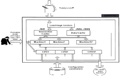
size

2.2.3.

Work

cycle of

the

SMT

SimOS/Topsy

environment

The

detailed

organizationof

the

SMT

SimOS/Topsy

integrated

environment

is

shown

in Figure 3.

J\ T'jpuy.i.'Cjff 1

J

L

*

Fvrsmjrinn mnrtn <>imul>1.ir lyFiM,r.PI I type. i

4>

Loacffmage function

.text -J

U

J U

.data,.rdata lriNliui:liiiri

Cm-.hi: grr

Udtu Cuchu

cJl^ *n*

_3fei^g

Tl>

\r.^ flfl.11:turn: 1 IUlMi:liirn*y MHi:hirn:MV

t:

X

X

It

,_ Configuration parameters

Figure

3.

fFor&

cyc/e

ofSMT

SimOS/Topsy

environment

The

user starts simulator

only

if

the

following

steps

have

been

completed:

1

.

SMT

Topsy

kernel

is built

using

the

MffSY

gcccross-compiler

2.

SMT

MXS

SimOS/Topsy

integrated

environment

is built

using Intel

gcc

compiler,

and

the

-DSMT option

is

present

in

the

Makefile

of cpus/mxs

subdirectory

of

the

simulator

[image:28.527.57.473.122.388.2]

The

user

then

enters

the

following

command

line in

the

simos root

directory:

Jsimos

-X

where-Xoption

indicates

that the

simulatorutilizes

the

MXS CPU

model.

Combined

with

CPU.Model

option,

this

commend

line

option

completely defines

the

simulated environment

(MIPSY

simulator/SMT

MXS CPU).

According

to

[32],

topsy.ecoff

file

contains

the

following

segments: .text

-text

segment of

the

kernel

(instructions),

_.data, .rdata

-data

segments of

the

kernel (variables

and constants).

After main()

function

completes

the

initialization

of

the simulator, the

simulator passes

the

control

to the

Loadlmage

function.

The Loadlmage

function is

responsible

for:

1)

extraction of

the

.text, .data, .rdata segments

from

the topsy.ecoff

file;

2)

loading

the

instruction

cache with

the

.text segment

data,

and

the

data

cache with

the

.data, .rdata

segments

data.

After

instruction

and

data

caches are

successfully

loaded

with

the

appropriate

data,

the

virtual machine

then

initializes

the

vector of

defined CPU

models

(in

this case, the

vector of

the

SMT

MXS

CPUs)

and calls

the

mscycleonce

function.

The

ms_cycle_once

function

implements

a single cycle of execution of a single

SMT MXS

CPU.

The

mscycleonce

function

calls ms_fetch

function,

which

implements

the

SMT MXS

fetching

unitand

is

one of

the

main emphases of

this

work.

In

addition, the

"SMT

MXS

Fetching

Unit"

section provides more

details

on

the

implementation

of

the

fetching

unit and

its

processing.

The

"Results"

2.3. Annotations

vs.

Performance Counters

According

to

SimOS

documentation,

annotationsaremechanisms

for

running arbitrary

TCL

scripts

throughout

the

execution of

the

simulation.

Annotations

are non-intrusive

mechanisms.

It

means

that

their

execution

does

not

necessarily

need

to

have any

affect on

the

behavior

of

the

workloadand

operating

systemunder simulation.

Annotations

are

triggered

by

any

number of

hardware

events,

including,

but

not

limited

to

execution of a specific

address,

loads

or stores

to

specific

data

locations,

device

interrupts,

and others.

In

addition

to

predefined annotation

types,

such as

discussed

above,

it is

also possible

to

create

user-defined

types

ofannotations.

These

are

typically

used

to

notify

scripts of

the

execution of

some

higher-level

event such as

the

creation of a new

process,

entering

idle

loops,

or

executing

a particular procedure

in

an application.

The

simulation uses

the

annotation

command

in both instances:

to

set annotations and

to

create new annotation

types

for

others

to

use.

Currently,

SimOS

supports

the

following

annotation

types:

Pc

-triggers

when

the

PC

equals a certain value and

fires

after all exceptions

caused

by

the

instruction's

execution and all cache misses

have

completed;

Load

-this

annotation

triggers

on

loads

to

aparticular

address;

Store

-triggers

on allstores

to

a particular

address;

Cycle

-triggers

when

the

cycle count reaches

the

predefined

value;

Exe

-

triggers

on exception of aparticular

type;

Inst

-triggers

when

the

instruction

of a particular

type

is

executed;

Simos

-triggers

on specific

SimOS

events;

Scache

-

triggers

on second

level

cache misses of a particular

type

or

any

type

if

the

type

is

not specified.

For

more

details

on

the

format

of annotation command please refer

to

SimOS

documentation

[26].

The

annotations approach

has

its

advantages and

disadvantages.

Among

the

advantages,

annotations provide

flexibility

and

low

execution

time

overhead.

One

of

the

disadvantages

of

using

the

annotation approach

is

a

necessity

to

have

multiple scripts

to

address

the

different

types

of

annotations,

inclusion

of

TCL

libraries

into

the

simulation

the

annotation approach

there

are

issues

related

to

installation

and

initialization

of

the

software related

to

the

specific

TCL

problems and versions

incompatibilities,

and

the

necessity

to

providespecial support of

TCL

in

the

software.

Taking

into

consideration

the

issues described

above,

a

different

approach

has

been

taken,

namely

performance counters.

The

performance counters

implemented in

this

work

somewhat mimic

the

Microsoft

approach.

Every

function in

simmxs

folder

writes

the

data in

the

series of

#

-

delimited

rows,

where

every

number

in

the

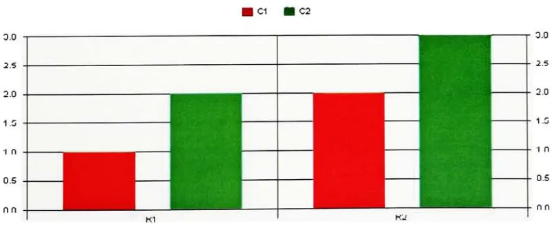
row represents a particular measured value of a particular matrix.

For

example,

if

some

data

measurements werewritten

by

function X for data

series

Cl

and

C2,

and

the

following

table

represents

the

actual [image:31.527.62.480.290.334.2]

measured

data:

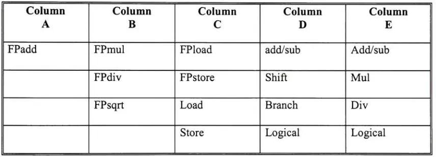
Table 2.

Viewing

data

with

RIT Viewer

application

Series

Cl

Series C2

i

1

2

2

3

Then

the

file

created

by

the

function X

will

look

like follows:

12#

2 3#.

A

special

Windows

application

RIT_viewer

was

developed

to

visualize

the

data.

Figure 4 demonstrates how RIT_viewer

interprits

the

data from

the

listed

above

file.

RIT

viewer

daLa

inLerpriLaLion

IC2 C1

3.0

2.0

1.0

K1 K2

2.0

[image:31.527.67.467.475.641.2]

The

idea is

that

the

function

returns some

data

that

is only

meaningful

to

the

interpreter.

That

allows

having

a single

display

for any

number of

totally

different

events.

Among

other

advantages, this

approach

introduces

a

truly

non-intrusive

coding

style; there

is

no need

to

support

any extra-libraries;

since counters are

implemented in

C,

any

environment

(including,

but

not

limited to,

TCL)

may

be

used

for display.

For

example, the

Windows

2000

performance

proxy

was used

to

monitor

the

simulation

running

on

the

UNIX

box

Chapter

3.

Developing

SMT MXS CPU

model

Section 3. 1

contains general specificationof

the

SMT MXS CPU

model.

Section

3.2

provides

detailed description

of

the

SMT

MXS

instruction

set.

Section 3.3

explains

the

organization of

the

SMT MXS

pipeline.

Section

3.4

provides

brief discussion

of

the

SMT

caches,

including

primary

instruction,

primary data

and

secondary

caches.

This

section also

describes

cache

algorithms and virtual-to-physical address

translation

process.

A brief discussion

of

the

operating

modes of

the

SMT MXS CPU

model

is

also provided

in

this

section.

Section 3.5

provides

detailed description

of

the

fetching

unit of

the

basic

MXS CPU

model;

it

then turns to

SMT

MXS

fetching

unit and

discusses

a

few

problems related

to

SMT

fetching

process,

as well as possible enhancements

to the

SMT MXS

fetching

unit.

Section

3.6

introduces

the

concept of register renaming.

The

section also

demonstrates

a

few

techniques

ofregister

renaming

that

are

implemented

in

the

SMT

MXS CPU

model.

Section

3. 7

explains

the

organization of

the

SMT MXS

issue

queues.

Section 3.8

contains

background

information

on

branch

predictionpolicies.

Section

3.9 describes

the

SMP MXS branch

predictionunit.

Section 3.10

introduces

a new

dynamic branch

predictionpolicy.

Section

3.11 illustrates

exception

handling

techniques

implemented

in

the

SMT MXS

CPU

model.

3.

1.

General

Description

Taking

a closer

look

at

the

SMT

shows

that the

SMT MXS

architecture can

be

categorized as

MIPS

V

(provided

that

a

typical

MIPS

architecture

has been

extended

four

times

and

the

basic R 10000

architecture

belongs

to the

MIPS

IV

category).

The

following

describes basic CPU

architecture

information,

as well as specific

SMT information.

The

detailed description

of

the

basic

architecture

is

contained

in

[r

10000

us.

Man].

The

specific

SMT

information is

referenced

according

to the

list

of sources.

The

SMT

MIPS

processor

is

a

single-chip

superscalar1

RISC

microprocessor

that

uses

MIPS

ANDES2 architecture and

has

the

following

major

features [5]:

1)

It specifically implements

the

64-bit

MIPS IV

instruction

set architecture

(ISA);

2)

It

can

decode

eight

instructions

each pipeline

cycle,

appending

them to

one of

three

32-entry

floating

point and

integer instruction

queues;

3)

It

has

ten

execution pipelines with

the

maximum

depth

of

9

stages connected

to

separate

6

integer

(including

4 Load/Store

and

2 Synchronization units)

and

4

floating

point

units;

4)

It

uses

dynamic instruction

scheduling3

andout-of-orderexecution4

;

5)

It

uses speculative

instruction issue (also

termed

"speculative

branching"

5);

6)

It

uses

non-blocking

caches

6;

7)

It

has

separate

on-chip 128-Kbyte primary instruction

and

data

caches;

8)

It

has

individually-optimized secondary

cache and

System

interface

ports;

9)

It

has

an

internal

controller

for

the

external

secondary

cache;

10)

It has

an

internal System

interface

controller with multiprocessorsupport.

The

table

below lists

the

parameters of

the

SMT

processorand

memory

system

that

are

Table 3. General

specification

of

SMT

microprocessor

Parameter

Description

Pipeline

9

stages

Fetch

Policy

8

instructions

percycle

from

up

to

2

contexts

(the

2,8

scheme of

[6])

Functional

Units

6 integer

(including

4

load/store

and

2

synchronization

units),

4

floating

pointunits

Instruction Queues

32-entry

integer

and

floating

point queues

Renaming

Registers

10