TO THE NUMERICAL SOLUTION OF DIFFERENTIAL EQUATIONS
by
G„A. Watson
A t h e s i s s u b mi t t e d t o t he A u s t r a l i a n N a t i o n a l U n i v e r s i t y f o r t h e de gr e e o f Doct or o f Phi l osophy
in collaboration with my supervisor. Dr. M.R. Osborne. Some of the results have been published in a number of joint papers, referenced Osborne and Watson (1967, 1969a, 1969b, 1969c), and these papers form the basis for
Chapters 2, 3 and 7 and Section 4.2 of Chapter 4. Where
parts of these papers consist of theorems and their
proofs, the text has been closely followed. The theorems
of Chapter 2 are largely the result of preliminary work by Dr. Osborne, prior to the commencement of my Ph.D. scholarship, and the proofs of many of the other theorems arose or were modified during discussion.
Elsewhere in the thesis, the work described is my
own and the numerical results I believe to be original,
I am p a r t i c u l a r l y i n d e b t e d t o D r . M. R. O s b o r n e f o r h i s p a t i e n t and e x p e r t s u p e r v i s i o n d u r i n g t h e t h r e e y e a r s i n w h i c h t h i s w o r k was d o n e . I w o u l d a l s o l i k e t o t h a n k D r . R . S . A n d e r s s e n f o r h i s c o n s t r u c t i v e c r i t i s c i s m as
r e g a r d s p r e s e n t a t i o n and M r s . S t e p h a n i e Larkharri / who p r e p a r e d t h e t y p e s c r i p t p a t i e n t l y and w e l l . I am a l s o g r a t e f u l t o M r . D. M. Ryan f o r h i s c a r e f u l r e a d i n g o f t h e t y p e s c r i p t / and t o M r s . Pam Hawke f o r h e r a s s i s t a n c e i n t h e t y p i n g o f t h e f i n a l v e r s i o n .
F i n a l l y I w o u l d l i k e t o t h a n k t h e A u s t r a l i a n
CHAPTER 1. INTRODUCTION 1
1„1 The approximation problem 5
1.2 Approximation on the real interval 8
1.3 Implicit function approximation 13
CHAPTER 2. THE DISCRETE T-PROBLEM 17
2 01 A survey of the classical theory 18
2.2 Linear programming and the Stiefel
exchange algorithm 25
CHAPTER 3. THE CONTINUOUS T-PROBLEM 39
3.1 A survey of the classical theory 39
3.2 The first algorithm of Remes 43
3.3 Linear programming and singular problems 46
CHAPTER 4. NONLINEAR MINIMAX APPROXIMATION 54
4.1 A survey of the theory 55
4.2 An algorithm for the discrete problem 61
4.3 An algorithm for the continuous problem 74
CHAPTER 5. MINIMAX APPROXIMATION OF EXPLICIT FUNCTIONS 78
5.1 Additional constraints 78
5.2 An example of a singular problem 82
5.3 Optimal starting values for /x 88
5.4 Rational approximation 90
NUMERICAL SOLUTION OF DIFFERENTIAL
EQUATIONS
99
6 01
Linear ordinary differential equations
101
6 0101
Increasing the number of unknowns
106
6 02
Nonlinear ordinary differential equations
111
6 0201 The general Thomas-Fermi equation
114
6 0202 The Blasius equation
118
6 0203 Simultaneous ordinary differential
equations
126
6 0 2 o4
Nonlinear boundary conditions
128
6 03 The eigenvalue problem for ordinary
differential equations
134
6 03 01
Linear eigenvalue problems
134
6 0302
Generalised eigenvalue problems
142
6 04
Partial differential equations
145
60401 The torsion equation in a rectangle
146
6 04 02
Laplace's equation
155
6 04 03
Laplace's eigenvalue problem for an
L-shaped region
159
CHAPTER 7 0
MINIMISING THE MAXIMUM ERROR IN THE
NUMERICAL SOLUTION OF ORDINARY
DIFFERENTIAL EQUATIONS
166
701 Linear equations
167
7*2 Nonlinear equations
172
703 A convergence result for the linear case
177
CHAPTER 1 INTRODUCTION
Approximation with respect to what is now known as the Chebyshev norm was proposed by Laplace (1799) in a study of the approximate solution of inconsistent linear equations» However/ the first systematic investigation of the problem
was carried out by Chebyshev (1854/ 1859/ 1881)0 The
mainstream of the early theoretical investigation was the study of a restricted subset of an important general class
of real linear problems. The members of this general class
fall naturally into one of two distinct/ though related types?
(a) the discrete problem/ which can be formulated as
a problem of solving an overdetermined set of linear equations/ and
(b) the continuous problem/ where a continuous
function (of one variable) is approximated on the interval [a/b] of the real line by a linear combination of continuous functions.
The 'classical theory' imposes strong conditions of non-degeneracy on these problems/ and the solutions of this restricted subset are extremely well-defined.
Significant contributions to this theory were made by
Apart from the contribution by Remes (1934, 1935),
and some interest in approximation in the complex domain
(for example Walsh (1935), Sewell (1942)), no further
important steps were made until the advent of electronic
computers, when the large scale computation of Chebyshev
approximations became possible.
This led to further
progress, in particular the development of theory for
linear problems not satisfying the classical requirements
(see, for example, Zuhovickii (1956), Cheney and Goldstein
(1959, 1962, 1965), Lawson (1961) and Rivlin and Shapiro
(1961)), although preliminary results were established by
Kirchberger (1903) and Young (1907),
Despite the attention given to these problems, the
classical assumptions have, until very recently (for
example Descloux (1961), Bittner (1961), Osborne and
Watson (1967)) continued to play an important role in
the actual computation of Chebyshev approximations.
The
work described in Chapters 2 and 3 of this thesis is a
contribution to the development of satisfactory techniques
for computing these approximations free from the
Chapter 2, which is based on the work by Osborne and Watson (1967), is devoted to a study of the linear
discrete problem» The classical theory is surveyed, and
an algorithm due to Stiefel (1959) is introduced» This
algorithm, which was developed within the framework of the classical theory, is shown to be equivalent to an algorithm based on a linear programming approach, the formulation of which is independent of the classical assumptions»
In Chapter 3, we consider the linear continuous
problem» Again, the classical theory is surveyed, and
the close connection with the classical theory for the
discrete case is illustrated» An algorithm due to Remes
(1935) is given which solves the general (non-classical) problem by considering a sequence of discrete problems» The use of linear programming to solve the discrete
problems appears to lead to difficulties when a certain
case of degeneracy occurs; this situation is clarified»
Since many of the problems which occur in practice are nonlinear, we have also considered the problem of providing reliable and generally applicable algorithms for the computation of the corresponding nonlinear
approximations» This is dealt with in Chapter 4» Results
converge under conditions which are often assumed to
hold in practice*
The remainder of the thesis is devoted to the
application of the theory and algorithms of Chapters 2,
3 and 4 to a large variety of problems0
Chapter 5 deals
specifically with the approximation of explicit functions,
while in Chapters 6 and 7 we consider an important
application to the approximate numerical solution of
differential equations* Two types of approach are
considered, both of which yield a wide range of non-
classical approximation problems*
A large selection of
differential equations, including partial differential
equations, is covered by the method of Chapter 6,
although the formulation of the method of Chapter 7 at
present only embraces the solution of ordinary
differential equations*
We begin by introducing some basic concepts and
notation from the general theory of approximation, with a
view to out1ining'the relevant existence and uniqueness
theorems* We then specialise to the particular case
with which we shall be concerned, viz* Chebyshev
approximation on the real interval or a finite subset of
it*
Further details, together with proofs of the stated
Ini Th e a p p r o x i m a t i o n p r o b l e m
D e f i n i 11 on 1 Let X be a set of e l e m e n t s (or points) and d a r e a l - v a l u e d f u n c t i o n d e f i n e d for all e l e m e n t s of X In such a w a y that the f o l l o w i n g hold for all x, y, z e Xs
( i ) d C x , x ) = 0
(II) d(x,y) > 0 If x ? y
(ill) d(x,y) = d(y,x)
( I v ) d (x , y ) < d (x , z ) + d (z , y ) 0
T h e n the set X and the d i s t a n c e f u n c t i o n or m e t r i c d t o g e t h e r d e f i n e a m e t r i c s p a c e .
On the b a s i s of this co n c e p t , the b a s i c p r o b l e m of a p p r o x i m a t i o n t h eo r y can be f o r m u l a t e d as f o l lows^
G i v e n a point g and a set M i n a m e t r i c space, d e t e r m i n e a point of M of m i n i m u m d i s t a n c e f r o m g 0
D e f i n i t ? on 2 S u c h a p o int is c a l l e d a be s t a p p r o x i m a t i o n . A best a p p r o x i m a t i o n m a y or m a y not exist, and
a s s u m i n g e x i s t e n c e , m a y or m a y not be u n i q u e 0 in general, such c l o s e s t p o i n t s do not e x i s t u n l e s s a d d i t i o n a l
a s s u m p t i o n s r e g a r d i n g the f o r m of the m e t r i c space, or a s u b s e t of it, are i n t r o duced« B a s i c to t h e s e a s s u m p t i o n s
6
.
D e f i n i t i o n 3 A s u b s e t K o f a s e t X I s s a i d t o be c o m p a c ti f e v e r y s e q u e n c e o f p o i n t s i n K has a s u b s e q u e n c e w h i c h c o n v e r g e s t o a p o i n t o f K 0
U s i n g t h i s c o n c e p t , we c a n s t a t e a b a s i c e x i s t e n c e t h e o r e m on t h e b e s t a p p r o x i m a t i o n i n a m e t r i c s p a c e .
Th e o r e m 1 . 1
L e t K d e n o t e a c o m p a c t s e t i n a m e t r i c s p a c e . Then t o e a c h p o i n t p o f t h e s p a c e , t h e r e c o r r e s p o n d s a p o i n t o f K c l o s e s t t o p .
The c o n c e p t o f a nor med l i n e a r s p a c e i s f u n d a m e n t a l t o t h e s t u d y o f many a p p r o x i m a t i o n p r o b l e m s ,
D e f i n i t i o n 4 L e t X be a s e t o f e l e m e n t s x , y , z , . . . f o r w h i c h a d d i t i o n and m u l t i p l i c a t i o n by s c a l a r s X, y , . . .
i s d e f i n e d . Then X i s a 1 i n e a r s p a c e i f t h e f o l l o w i n g a x i o m s a r e s a t i s f i e d :
( i ) x + y e X
( i i ) x + y = y+x
( i i i ) x + ( y + z ) = ( x + y ) + z
( i v ) X . x e X
( v ) X . ( y . x ) = ( X . y ) . x
( Vi ) (X + y ) . x = X. x + y . x
De f t n i 1 1 on 5 A r e a l - v a l u e d f u n c t i o n w h i c h i s d e f i n e d on t h e e l e m e n t s x , y , . . . o f a l i n e a r s p a c e X i s c a l l e d a nor m o f X and i s d e n o t e d b y | | x | | , | | y | | , . . . i f i t s a t i s f i e s t h e c o n d i t i o n s
( i ) I I x I I > 0 u n l e s s x = 0
( i i )
I I
x xI I
=I x l
I I x |I
w h e r e \ i s a s c a l a r ( M i ) I I x + y I I i ! I x I I + I I y I I 0A l i n e a r s p a c e f o r w h i c h a nor m i s d e f i n e d i s c a l l e d a nor med l i n e a r s p a c e . I n a nor med l i n e a r s p a c e , t h e f o r m u 1 a
d ( x , y ) = I I x - y | | ( 1 . 1 )
d e f i n e s a m e t r i c , as can e a s i l y be s h o wn .
An i m p o r t a n t e x i s t e n c e t h e o r e m f o r l i n e a r s p a c e s i s
T h e o r e m 1 „ 2 R i e s z ( 1 9 1 8 )
A f i n i t e d i m e n s i o n a l l i n e a r s u b s p a c e o f a nor med l i n e a r s p a c e c o n t a i n s a t l e a s t on e p o i n t o f mi n i mu m d i s t a n c e f r o m a f i x e d p o i n t .
De f ? n i t i o n b L e t X be a nor meu l i n e a r s p a c e w i t h x , y e X. Then i f
I l x | I = I I y I I = I I ± ( x + y ) I I ( 1 . 2 ) i m p l i e s t h a t x = y , t h e n X i s s a i d t o be s t r i c t l y c o n v e x .
Theorem 1 . 3 K r e i n ( 1 9 3 8 )
In a s t r i c t l y convex normed l i n e a r s p a c e , a f i n i t e d i m e n s i o n a l s ubspace c o n t a i n s a u n i q u e p o i n t c l o s e s t t o any g i v e n p o i n t . ,
1„2 A p p r o x i m a t i o n on t h e r e a l i n t e r v a l
L e t B be a compact space and d e n o t e by c[bJ t h e l i n e a r space o f c o n t i n u o u s r e a l - v a l u e d f u n c t i o n s d e f i n e d on B0
Def i n i t i on 7 L e t f e C [ß] . Then we d e f i n e t h e norm by
I 1 f 1 I = xm®XB l f ( x ) | . ( 1 . 3 )
T h i s i s t h e Chebvshev norm ( s o me t i mes c a l l e d t h e maximum norm or u n i f o r m norm)»I
We w i l l be p a r t i c u l a r l y c o n c e r n e d w i t h a p p r o x i m a t i o n pr ob l e ms wher e B i s t h e r e a l i n t e r v a l [ a , b j o r a f i n i t e
d i s c r e t e s u b s e t o f i t . C o n s i d e r t h e pr o b l e m o f a p p r o x i m a t i n g t o a c o n t i n u o u s f u n c t i o n f ( x ) i n t h e r a n g e j a , b j by a
l i n e a r c o m b i n a t i o n o f p c o n t i n u o u s f u n c t i o n s <J>^(x), « ^ ( x ) , . » . . <j>p ( x ) e T h i s can be f o r m u l a t e d as:
f i n d a v e c t o r a = ( a . . , a 0 , . . 0, a )"*" wh i c h m i n i m i s e s
r \j ± z. p
P
(We will distinguish vector quantities throughout this thesis
by the underlining Any vector a is assumed to be a column
%
vector; the superscript ^ denotes the transpose).
This problem is called a 1 inear continuous minimax approximation problem or (linear) continuous T ° p r o b 1em
If we replace the interval £a,b3 by a discrete set of values X j , j = 1 , 2 , . 0 „, n>p, a < Xj < b, then we define the prob 1em:
find a to mini m i s e
^
P
max I f (x . ) - E a <J). (x.) |, j=l,2,...,n
j
i=i
1
1
j
(1.5)
DefInition 9 This problem is called a 1 inear discrete
minimax a pproximation problem or (linear) discrete T-problem corresponding to (1.4).
Definition 10 Solution vectors a to the problems ( 1 04)
and (lo5) are called mini max
The discrete problem (1.5) is an approximation problem with respect to the vector norm defined on
x ( x 2 * x 2 f
'
V by
I IxI I = max Ix.I, i=1,
2
,Remark 2 Although the existence of solutions to these problems is guaranteed by Theorem 1,2, we cannot guarantee uniqueness without imposing additional
assumptions, (It is shown in Chapters 2 and 3 that these
are in fact the classical assumptions.)
Def ? nition 11 The minimum value of the norm defined by
equation (1.3) is called the min max d e v i a t i o n .
It is reasonable to suppose that if the discrete set
of points Y = {y j } somehow fills out the interval A =
[a,bj , then the min max deviation of the discrete problem will approximate in a sense to the min max deviation of
the continuous problem.
Definition 12 The dens ? tv of Y in A is defined by
I Y I max inf
6 e A y
e
YIy~6I .
Theorem 1.4 Motzkin and Walsh (1956)
If f (x ), <f>.(x) e C [aJ , i =1, 2, . . ., p ,
min max
a y e Y
P
I f (y ) — Z a . <J>. (y) | -► i “ 1
min max , . * £ . , x . ,
a 6 e A lf («>- E a.<t>. («) I
For nonlinear approximation problems/ the parameters
to be determined enter nonlinearly. Consider the problem
of approximating to a continuous function f(x) by a
continuous function F(X/ ct^/ ot^/ •••/ a p ) in the range
j^a/b]. This can be stated:
find a = a a )^ to minimise
% i. C. P
max I f(x) - F(X/a) \ , a £ x £ b . (1.6)
%
This is the nonlinear problem corresponding to (1.4).
If we consider the discrete set of values x.7
J
j=l/2,00./n / a < (x.) < b/ then the problem j
find a to minimise
'V
max I f(x.) - F(x./a) | / jssl/2/ .../n (1.7)
J J *\j
is a nonlinear problem corresponding to (1.5). It is also
a discrete problem corresponding to (1.6).
Remark 5 On the basis of Theorem 1.1/ the existence
of solutions can only be guaranteed if the set of
approximating functions F(X/Cx) is compact. Though this is
not generally true/ it is often assumed in practice that the search for a best function is confined to a compact
11
.
Remark 4
Further conditions on the functions F(x,a)
are required to ensure uniqueness«
These are discussed in
detail in Chapter 4.
A theorem, similar to Theorem 1.4, can be given for
nonlinear approximation«
The proof is similar to that for
the linear case given in Cheney (1966).
Theorem 1,5
Let Y and A be defined as before
f(x), F(x,a) e C [
a^ ,
Then if
min max
a y e
%
Y I
f (y) - F(y,a)| - m ^n ^
A |f(6) - F(6,a)| ,
a
as
I
Y I
0 .
Proof
Let 6 e A and y e Y be such that
I
6 - y I
< e.
If
n(e,a)
max
1
6~y1
< e
1
F ( 6 / a ) - F (y, a ) 1
%
and
W
(e)
=
sup
|
6
—
y |
< e 1
f (6)
f (y) 1
then by the continuity of F and f,
n (e,cO -
0
a s e +o ,
and
w
(e )-
*
•
0as
e -
*
■
o .
Now let
min max
a y e Y
I f (y) “y T y lf(y) " F(y^ }|-
I l f - F(0) I
I
y,
'V '
/
and m i n max | f ( ö ) - F ( 6 / a ) | = max | f (<5) - F ( 6 , y ) |
a 6 e A % 8 e A %
= I I f - F (y) | | A , s a y »
Then
I l f - F ( 3 ) I Iy < I l f - F (y) 1 l A ( 1 . 8 )
I f 6 e A i s s u c h t h a t | f ( 6 ) - F ( 6 / B) | i s a maxi mum/
* \ j
and y e Y i s s u c h t h a t
16 - y I < e / t h e n
I l f - F ( y ) | | = m‘ ° I I f - F ( a ) I I.
% A a ^ A
< I I f - F ( 3 ) I l A
= I f (6 ) - F (6 / 3 ) I 'V
< I f ( 6 ) - f ( y ) I + I f ( y ) - F ( y , 3 ) I
'Xj
+ I F ( y / 3 ) - F C 6 / 3 ) |
' V ^
< W( e) + | | f - F ( 3 ) I I v + n ( e / 3)
v a
,
*
<\j( 1 . 9 ) T h u s , f r o m ( 1 . 8 ) and ( 1 . 9 ) we ha v e
I l f - F ( 3 ) I I y - I l f - F ( y ) I I a as e - 0 , s i n c e b o t h W( e ) and f t ( e , 3 ) 0 as e -► 0 0
T h i s c o m p l e t e s t h e p r o o f 0
1 . 3 I m p l i c i t f u n c t i o n a p p r o x i m a t i o n
I n t h e p r e c e d i n g s e c t i o n / we f o r m u l a t e d c o n t i n u o u s and d i s c r e t e a p p r o x i m a t i o n p r o b l e m s f o r e x p l i c i t l y d e f i n e d
M( y ( x ) ) = f ( x ) , a < x < b , ( l o1 0 ) w h e r e M i s an o p e r a t o r , y ( x ) i s t h e f u n c t i o n t o be
a p p r o x i m a t e d , a n d f ( x ) e c [ a , b ] .
T h o u g h we s h a l l n o t a s s u m e t h a t ( 1 . 1 0 ) h a s a n a n a l y t i c s o l u t i o n , we s h a l l deman d t h a t t h e c o r r e s p o n d i n g p r o b l e m i s w e l l - p o s e d . O f t e n y o r i t s d e r i v a t i v e s w i l l be r e q u i r e d t o
s a t i s f y c e r t a i n s u b s i d i a r y c o n d i t i o n s .
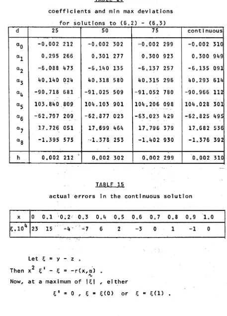
D e f i n ? t i o n 13 I f z ( x , a ) i s an a p p r o x i m a t i o n t o y c o n t a i n i n g
'V.
f r e e p a r a m e t e r s a ^ , o ^ / . . . / a p/ t h e n t h e f u n c t i o n
£ ( x , a ) = y ( x ) - z ( x , a ) ( 1 . 1 1 )
'V %
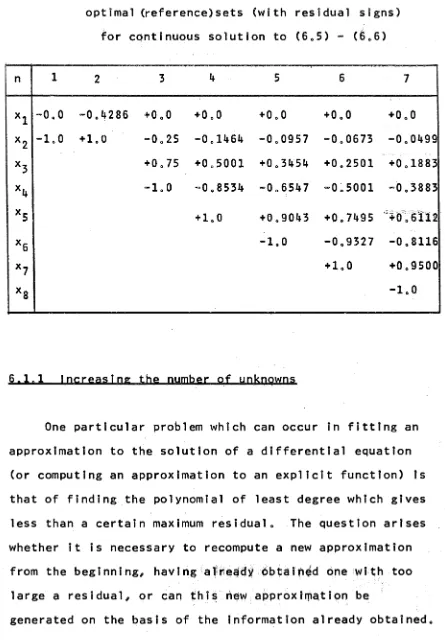
i s c a l l e d t h e e r r o r o f t h e a p p r o x i m a t i o n . T h e f u n c t i o n r ( x , a ) ■ M ( z ) - M ( y ) ( 1 . 1 2 )
%
i s c a l l e d t h e r e s i d u a 1 .
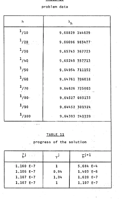
We w i l l be p r i m a r i l y c o n c e r n e d i n t h i s t h e s i s ( w i t h t h e e x c e p t i o n o f C h a p t e r 7 ) w i t h o b t a i n i n g a p p r o x i m a t i o n s t o y w h i c h m i n i m i s e t h e ma x i mu m v a l u e o f t h e r e s i d u a l r ( x , a ) . S u c h a p p r o x i m a t i o n s w i l l be c a l l e d m i n i max r e s i d u a l s o l u t i o n s . P r o b l e m s o f t h i s t y p e c a n be
f
K
(x,t) y(t) dt = Xy(x) + f(x), a < x < b, to
where X is a constant, and K, y and f are continuous in the region of interest.
Suppose that we wish to approximate to y(x) by z = z(x,a) where
p 'v
z = E a. 4>. (x),
i =1 1 1
and where the functions 4>.(x)
e
C[a,b] are prescribed.Then from equation (1.12) we have
P tn p
r(x,a) = X E a.4>.(x) + f(x) - / K(x,t) E a.<J>.(t)dt
i=l 1 1 t i =1 1
o P
= E a.ijj.(x) + f(x), (1.13)
i =1
where i
|
j.(
x)
= X . (x ) + / K(x,t) 4>.(t)dt , i=l,2,00.,p tMore generally, we have
r(x,a) = M(z) - M(y) = F(x,a) - f(x) (1.14)
where F(x,a) is nonlinear in the elements of the vector a
% 'V
Thus, we see that the problem of obtaining a minimax residual solution to an operator equation of the form
(1.10), assuming that z is suitably chosen, is a continuous
minimax approximation problem. It will be a linear problem
CHAPTER 2
THE DISCRETE T-PROBLEM
In this chapter, we investigate how the restrictions of classical linear approximation theory affect techniques for computing linear discrete minimax approximations to
functions» We establish the equivalence of the Stiefel
exchange algorithm (Stiefel, 1959), which was developed largely within the framework of classical a p p r oximation theory, with an algorithm based on a linear programming approach, and show that the linear programming algorithm
is free from the usual restrictions imposed on the Stiefel exchange algorithm»
Notation The following standard notation is used»
We wri t e P.(A) and Kj(A) for the i ^ row and the column
respectively of the matrix A„ The unit vector e. is
'VJ
4- l_
defined as usual to be a vector with 1 in the j place and
zeros elsewhere» We write e for the vector each element
of which is 1» The standard notation for partitioned
vectors and matrices is used - for example is a column
f X ~1T
vector X extended by a scalar t, and the row vector
2.1 A survey of the classical theory
The discrete T-problem can be regarded as the problem of finding a vector a to minimise
max |
' r i 1 , i « 1,2,. . .,n
where r
'V.
* f - A a.
% 'V (2.1)
Remark 1 In this chapter, we treat the general
discrete T-problem, of which (1.5) is a special case.
If the matrix A is (nx p) where p < n, then the
classical results concerning the solution of this problem are based on the assumption that the matrix A satisfies the Haar cond ? tion.
Definition 1 If every (pxp) submatrix of A is nonsingular,
we say that A satisfies the Haar condition. In order to
explain the significance of this condition, it is convenient to introduce the following definitions.
Definition 2 Any set of (p+1) equations of (2.1) is
called a reference. The corresponding submatrix is written
Ag and the components of f and r associated with the
reference form vectors which are written f ° and rG
'V %
19 .
Defini11 on 3 By the Haar condition, the rank of A° is p 0
Therefore, there is a unique vector (up to a scalar multiplier) satisfying the equation
XT A° = 0 (2.2)
'V
This vector is called the X-vector for the reference,. It is clear that all components of X are different from
'V, z e r o .
Definit ? on 4 The vector a is called a reference vector
'V
if either
sgn(r.C ) 53 sgn(X.) , i =1,2, .. „, p+1 ,
or sgn(r.°) ** -sgn(X.) , ? « 1 , 2, . . ., p+1 .
Definition 5 Let g be the vector defined by
'V
g s g n (A •) ,
i*1,2,...,p+1 .
Then the matrix (A |^) is nonsingular so that the
vector
ß
is uniquely defined by the equations.a
A a f
a, (2.3)
In this case, a is called the levelled reference vector and h is called the reference d e v i a t i o n ,
Theorem 2.1
20
.
P r o o f Let t h e r e f e r e n c e , l e v e l l e d r e f e r e n c e v e c t o r and r e f e r e n c e d e v i a t i o n be d e f i n e d by e q u a t i o n ( 2 . 3 ) . Then i f X i s t h e X - v e c t o r f o r t h i s r e f e r e n c e ,
< \j
XT f ° ^ %
P+1 h I
i =1
I X. I ( 2 . 4 )
Now, l e t a be any o t h e r v e c t o r such t h a t %
.a * A a
%
..a a
f - r , wher e
Then
max I r . | , i * 1 , 2 , . . . , p+1
_ p + l p + l
AT f a = A r £ I I A . I I r . 0 1 £ h* | A . | ( 2 . 5 ) % ^ % %j K x I I i = l 1
E q u a t i o n s ( 2 . 4 ) and ( 2 . 5 ) g i v e h * h* ,
and s i n c e t h e Haar c o n d i t i o n e n s u r e s t h a t a l l component s o f X a r e n o n - z e r o , e q u a l i t y can o n l y h o l d i n t h i s e q u a t i o n
i f
( i ) I r -° I a h* , i - 1 ,2 , . . . , p + l , and ( i i ) s g n ( r . a ) * g. i = 1 , 2 , . . . , p + l .
ft
Thus a i s a l e v e l l e d r e f e r e n c e v e c t o r , and so *
a = a
' V 'Vy
by t h e u n i q u e n e s s r e s u l t ( D e f i n i t i o n 5 ) .
T h i s c o m p l e t e s t h e p r o o f .
de la V a l l e e P o u s s i n C1911)
The m i n i m a x s o l u t i o n of e q u a t i o n s ( 2 01) is a l e v elled r e f e r e n c e v e c t o r for some r e f e r e n c e 0 Further, m a x l r ^ l * h, w h e r e h is the r e f e r e n c e d e v i a t i o n for this r e f e r e n c e ,
Th e Haar c o n d i t i o n is s u f f i c i e n t for the v a l i d i t y of this theoremo
Lemma 2 „1
If the m a t r i x A s a t i s f i e s the Haar c o n d i t i o n , then a s o l u t i o n to the d i s c r e t e p r o b l e m is isolated»
This is the linear case of Lemma 4 03 0
Lemma 2 „2
if the m a t r i x A s a t i s f i e s the Haar c o n d i t i o n , then the s o l u t i o n to the d i s c r e t e p r o b l e m is u n ique»
is also a s o l u t i o n »
This c o n t r a d i c t s Lemma 2»1, and so the s o l u t i o n is unique»
T h e Haar c o n d i t i o n is a l s o s u f f i c i e n t for the v a l i d i t y of the f o l l o w i n g result»
Let a = ß and a = y be d i s t i n c t s o l u t i o n s to the p r o b l e m C 2 01)„ I K T h e n it is e a s i l y seen that
a ■
2
2
.
Theorem 2 „3
Stiefel (1959)
Given any reference and a corresponding reference
vector, then it is possible to add to the reference any
other equation and to drop an appropriate equation from
the reference so that the given vector is also a reference
vector for the new reference.
Proof
(This proof is given in Watson (1966), and is
essentially an extension of the derivation given in Stiefel
(1959) for the case ps3).
If p^(A) is the row to be added to the current
reference, then, by the Haar condition, the matrix
o
(2.6 )
A
pk(A)_
has rank p.
There are therefore two linearly independent
vectors v
0, 0,1
v, and v 3 v0 such that
o,
V T
M
o,
(2.7)
(o)
One such vector is
where A NW/ is the
A-vector for the current reference, so that any vector
satisfying (2.7) must be expressible in the form (to
within a scalar multiple)
(o)'
u
0
,
A
o,
0
0,
V(
2
.
8
)
where v
is any’
solution of equation (2.7) which is not a
o,
computationally convenient satisfies p+I
s g n (r k ) p k (A) + z
i
=1
v . p . (A ) C 2 o 9 )
but it could, for example, be chosen to be orthogonal to (o)T
Now let a be a reference vector for the current
%
reference« Then M a
%
and it can be arranged that
Ci) X . (o) (r ° ). > 0, i=l,2,.„.,p+l,
% 1
r a "
r a l
f° r %
'V
— 1 4 -1 (2.10)(ii) v p + 2 rk > 0 ^see f ° r example equation ( 2 09 ) ) 0
If, for some value of j, we choose (o)
Y
Vo / XJ J
(
2
.
11
)
then u . s 0 and the remaining components of u form the
J 'v
4.
X“ vector for the reference obtained by deleting the j row
of Mo if a is to be a reference vector for this new
reference, then we must have
u.(r°). = ((r ° ) . X . (o))(y + v . / X . ( o ) ) > 0
% %
i
fj, i=1,2,0 0 «,p+1
(2.12)This inequality is satisfied provided j is the index of the algebraically least among the quotients v./X.^°^,
i = 1 , 2 , «««, p+1, and this proves the theorem« The Haar
Remar k 2 F o r c o n v e n i e n c e i n m a k i n g c o m p a r i s o n s w i t h t h e r e s u l t s o f t h e n e x t s e c t i o n , n o t e t h a t i f u i s d e f i n e d
%
by
u
( o )
Y v
t h e n t h e a p p r o p r i a t e v a l u e o f y i s e q u a l t o t h e l e a s t i n m o d u l u s among t h o s e q u o t i e n t s w h i c h a r e n e g a t i v e T h i s i s o b v i o u s l y a n o n - e m p t y s e t when v i s o r t h o g o n a l t o
%
( ° ) T ^1 w j f o l l o w f r o m t h e r e s u l t s o f t h e n e x t s e c t i o n t h a t i t i s n o n - e m p t y when v i s d e f i n e d b y e q u a t i o n
'V
( 2 . 9 ) .
T h e o r em 2 . 3 p r o v i d e s a b a s i s f o r t h e c o m p u t a t i o n o f t h e m i n i m a x s o l u t i o n 0 I n an a c t u a l c o m p u t a t i o n , t h e c h o s e n r e f e r e n c e v e c t o r w o u l d be t h e l e v e l l e d r e f e r e n c e v e c t o r f o r t h e g i v e n r e f e r e n c e , and t h e e q u a t i o n t o be a d d e d w o u l d be t h a t a s s o c i a t e d w i t h t h e c o m p o n e n t o f maxi mum m b d u l u s o f I f t h i s e q u a t i o n i s i n t h e r e f e r e n c e , t h e n t h e c o m p u t a t i o n i s c o m p l e t e d . I t i s r e a d i l y shown t h a t t h e m a g n i t u d e o f t h e r e f e r e n c e d e v i a t i o n r i s e s m o n o t o n i c a l 1y . L e t t h e
i n d i c e s o f t h e e q u a t i o n s i n t h e r e f e r e n c e be ° 00' Gp + l
l e t j be t h e i n d e x o f t h e e q u a t i o n t o be a d de d and l e t a . be t h e i n d e x o f t h e e q u a t i o n t o be d r o p p e d
e q u a t i o n s ( 2 04 ) and ( 2 . 5 ) ,
T h e n , by
( n )
Z i
4
iI Cn) | | h ( o ) , + ) x ( n ) , j r j
• J J
P+1
z
i =1
IX
( n )> | h < 0 ) |
( 2 . 1 3 )
«
?
p r o v i d e d that |Tj| > |h(o) The s u p e r f i x e s n and o refer to the old and new r e f e r e n c e s r e s p e c t i v e l y Q As t h ere are o n l y a f i n i t e n u m b e r of refere n c e s , a s o l u t i o n is f o u n d in a f i n i t e num b e r of s t e p s Q This a l g o r i t h m is c a l l e d the St i e f e l e x c h a n g e a l g o r i t h m »
near p r o g r a m m i n g and the Stiefel e x c h a n g e a l g o r i t h m
In this section, s t a n d a r d results from linear p r o g r a m m i n g t h e o r y are used.. T h e text f o l l o w e d is
H a d l e y (1962), and r e f e r e n c e s to this will be c i t e d w h e r e a p p r o p r i a t e in the form ( H 0 page no»)»
The d i s c r e t e T ~ p r o b l e m ( 2 01) can be posed as a linear p r o g r a m m i n g problem» To see this, let
T h e n the s o l u t i o n is o b t a i n e d by m i n i m i s i n g h s u b j e c t to
One of the f i rst to c o n s i d e r the linear p r o g r a m m i n g f o r m u l a t i o n of this p r o b l e m was Z u h o v i c k i i (1950, 1951, 1953)»
T h e m a t r i x f o r m of this linear p r o g r a m m i n g p r o b l e m is
h = m a x Ir jI , i=1,2
h - r s
I
0 ,(2.14)
h ♦ r. ^ 0
T a
m i n i m i s e Z 88 e ^
s u b j e c t to h ^ 0
' — —i i
A e a f
% and
“ A e h
l
-f %
w h e r e e q u a t i o n ( 2 01) has b e e n u s e d 0
C 2 o16)
T h i s f o r m is not p a r t i c u l a r l y s u i t a b l e for the
a p p l i c a t i o n of s t a n d a r d t e c h n i q u e s b e c a u s e the m a t r i x of c o n s t r a i n t s is 2n x (p+1), so that 2n s l a c k v a r i a b l e s
(Ho
Po 72) are required, and b e c a u s e the c o m p o n e n t s of a are not c o n s t r a i n e d to be p o s i t i v e » Th i s latterd i s a d v a n t a g e can be c i r c u m v e n t e d by e l i m i n a t i n g the e l e m e n t s of a in terms of the s l a c k v a r i a b l e s (Watson, 1 9 6 6 ) 0 However, both t h ese d i f f i c u l t i e s can be o v e r c o m e by t u r n i n g to the dual p r o g r a m (H» p» 2 2 1 ) 0 Here, the dual c o n s t r a i n t s , w h i c h c o r r e s p o n d to c o l u m n s of the o r i g i n a l (primal) p r o b l e m a s s o c i a t e d w i t h the
u n c o n s t r a i n e d v a r i a b l e s are e q u a l i t i e s CH»
P»
238), and all the dual v a r i a b l e s are c o n s t r a i n e d to be p o s i t i v e( H 0 p. 2 3 6 ) 0 T h e a d v a n t a g e g a i n e d by u s i n g the dual of the linear p r o g r a m m i n g f o r m u l a t i o n of the a p p r o x i m a t i o n p r o b l e m seems to h a v e be e n p o i n t e d out f i r s t by K e l l e y
The dual programming problem is
m a x i m i s e z = [ Y L - f T l W
L'v % J ( 2 . 1 7 )
s u b j e c t t o w 'l
'V 0
a n d
t*T <*> o II 2 c" < 1 8
( 2 . 1 8 )
U T
-e T ] w £ 1,
% j ( 2 . 1 9 )
Only one slack variable has to be added to equation
( 2 019) to make all constraints equalities., However, use
of the simplex method of Dantzig (1951) to solve this
problem requires the addition of p artificial variables to set up the initial basis matrix ( H 0 p 0 1 1 6 ) 0
Lemma 2.3 Osborne and Watson (1967)
An optimal (feasible) solution ( H 0 p a 6) to the system ( 2 017) - ( 2 019) with a non-zero slack variable is possible only if w = 0 0
Proof
constraints ( 2 C18)
With the addition of the slack variable w g , the C 2 o19) become
e e
%
0
%( 2 o 2 0 )
Assume that
w f 0, and define
s '
w
w
a-s an optimal a-solution with w f 0
2n
Z w
i =1
This v e c t o r s a ti s f i e s all the c o n s t r a i n t s on the problem, and gives the o b j e c t i v e f u n c t i o n z the f o l l o w i n g va 1 ue
"""I
1
Wr T J.T n %
Z “ 2n
l
*’ 1
' 0I w . — —
LO j
„ — — —
w
f T , - f T , o 'V
w
u -J s _
because, by the last e q u a t i o n of ( 2 0 2 0 ) , 2n
2 w. < 1 , if w j* Oo
i =1 1 s
This c o n t r a d i c t s the h y p o t h e s i s that opt i m a l s o l u t i o n 0
i s an
R e m a r k 5 If w « 0 is an optimal s o l u t i o n , then
h = Z = z = 0 ,
so that, by e q u a t i o n s ( 2 014),
r » = 0, i = l , 2 , 0 0 0 , n„
This implies that the or i g i n a l set of e q u a t i o n s has an exact solution,, We s p e c i f i c a l l y e x c l u d e this case f r o m c o n s i d e r a t i o n and thus
assume w
■0
and d r o p thev s
Lemma 2 „ 4 O s b o r n e and Wa t s o n ( 1 9 6 7 )
- max 1f o 1 < z < max | f . | , i = 1 , 2 , 0 » 0/ n„
P r o o f E q u a t i o n (2 017) g i v e s
z = f f T , - f T ”| w < max | f . I £ w
L 'v 1 | =1
= max I f . I ,
s i nee | e"^, e"^ I w « 1 „ L'v ^ J 'v
S i m i l a r l y - max | f . | < z 0
Remark 4 T h i s shows t h a t t h e r e g i o n o f p o s s i b l e v a l u e s o f z i s b o u n d e d 0
Lemma 2 . 5 O s b o r n e and Wa t s o n ( 1 9 6 7 )
C o n s i d e r t h e a p p l i c a t i o n o f t h e s i m p l e x a l g o r i t h m t o t h e s y s t e m (2 017) - ( 2 01 9 ) 0 Then i f an y c o l u m n o f
V
and t h e c o r r e s p o n d i n g c o l u m n o fV
a p p e a r t o g e t h e rT T
$ . - * \ej '
i n t h e b a s i s , t h e c u r r e n t v a l u e o f z < 0„
P r o o f C o n s i d e r t h e T ~ p r o b l e m o b t a i n e d by d e l e t i n g a l l e q u a t i o n s e x c e p t t h o s e r e l a t i n g t o c o l u m n s i n t h e d u a l b a s i s » The s e t w h i c h r e m a i n s c o n t a i n s a t m o s t p
e q u a t i o n S o L e t t h i s p r o b l e m be s o l v e d by a p p l y i n g t h e s i m p l e x a l g o r i t h m t o t h e d u a l p r o g r a m . Then t h e o p t i m a l
T
b a s i s f o r t h i s p r o b l e m c o n t a i n s a c o l u m n o f H and t h e
Now if a column is in the optimal basis for the dual, the corresponding equation in the primal is an equality
(H. p„ 239). Therefore, for at least one i,
h + r. = h - r j ä 0,
whence h = 0. Therefore, the optimum of the reduced
problem is z 6 0 and so z £ 0 for the current basis.
Remark 5 Since this case has been specifically
excluded from consideration, progress can only be made towards a solution by dropping one of the duplicated
columns from the basis, and a stage must be reached where
they are absent. We shall assume that no basis contains
columns duplicated in this way.
We shall now demonstrate that the simplex algorithm applied to the dual linear program is equivalent to the
Stiefel exchange algorithm. This result is contained in
Stiefel (1960). However, Stiefel eliminates the
unconstrained variables from the primal before proceeding to the dual, and his argument is largely geometric and
carried out for a small number of variables. We have
already shown that the elimination of the unconstrained variables is unnecessary.
By Remark 5, the columns of equation ( 2 0 2 0 ) which form the basis correspond to a reference for the original T-problem.
In the simplex algorithm each basis matrix must be
nonsingular and for this it is both necessary and sufficient for the matrix AG associated with the corresponding
reference to have rank p 0 Note that the first p equations
of (2 „ 2 0) express a relation of linear dependence between the rows of the reference while the last equation can be
interpreted as imposing a scale. As Aa has rank p, this
relation of linear dependence is unique/ and an immediate consequence of this is
Lemma 2.6 Osborne and Watson (1967)
The non-zero components of a basic feasible solution w are equal in modulus to the appropriate components of
the A-vector for the corresponding reference. The A-vector
is scaled so that the sum of the moduli of its components is o n e .
Remark 6 The Haar condition is sufficient for the
existence of a basis for the simplex algorithm but it is clearly much stronger than necessary.
Remark 7 To each reference there corresponds two
distinct bases for the dual program. Each basis determines
values of z are opposite in signQ As the optimum value of
z is positive, this defines the basis of interesto This
corresponds to choosing the A-vector so that A. r. \ 0 o
Lemma 2 „7 Osborne and Watson (1967)
The value of z given by the basic feasible solution is equal to the reference deviation for the corresponding reference»
Proof From equation (2017)
which, by Lemma 2 C6
t
P+i
- If XI / I |X. I
'V
J = 1
1
= IhI , by equation ( 2 0 4 ) 0
Remark 8 Lemmas 2 06 and 2 07 show that the current
basic feasible solution provides a solution to the T- problem for the current reference,.
Lemma 2 „8 Osborne and Watson (1967)
The choice of the vector to enter the basis in the simplex algorithm is equivalent to the choice of the
Proof
cT
fT , -f‘
a,
%
let B be the basis m a t r i x , and let c D be the v e c t o r
o b t a i n e d from c by d e l e t i n g the c o m p o n e n t s c o r r e s p o n d i n g to the n o n b a s i c ve c t o r „ Further*, let
/
^ ß T B '=1 K S
V
1-T
e e
%
sBl,2*ooo#2n
(2 o 2 2)
Now, if a c o lu m n is in the optimal dual basis, then the c o r r e s p o n d i n g e q u a t i o n in the primal is an e q u a l i t y
(Ho p 0 239), By R e m a r k 8, the c u r r e n t b a s i c f e a s i b l e s o l u t i o n solves the T = p r o b l e m for the c o r r e s p o n d i n g
r e f e r e n c e and h e n c e is op t i m a l for this r e s t r i c t e d problem.
T h e r e f o r e (B” 1 ) T
( 2 0 23 )
w h e r e a is the l e v e l l e d r e f e r e n c e v e c t o r and h is the r e f e r e n c e d e v i a t i o n for the c u r r e n t refe r e n c e ,
+ P
T h e r e f o r e z 83 h - E A, a (2,24)
S q=l jq Q
w h e r e j = s and the + sign is a p p r o p r i a t e if s £ n, o t h e r w i s e j « s~n and the - sign is taken. By E q u a t i o n
(2,1), this is e q u i v a l e n t to
s h + r . + c
The new c o l u m n t o e n t e r t h e b a s i s i s t h a t a s s o c i a t e d w i t h t h e l a r g e s t p o s i t i v e v a l u e o f c g - z g ( H 0 p Q 1 1 1 ) 0
Now,
c ~ z = » r . - h ( 2 o 26)
s s j
so t h a t t h e v a l u e o f r» o f maxi mum m o d u l u s d e t e r m i n e s s G J
T h i s c o m p l e t e s t h e p r o o f 0
Remar k 9 From e q u a t i o n ( 2 . 2 6 ) , t h e c o l u m n t o be a d de d t o t h e b a s i s i s
s g n ( r . ) k o ( A T )
j j
1
and t h i s i s e x p r e s s i b l e i n t h e f o r m (H s g n ( r . ) k. CAT )
j j
1
Po 85)
p>i
E y . k. ( B )
i-i
1 1( 2 o 2 7)
Lemma 2 „ 9 O s b o r n e and Wa t s o n ( 1 9 6 7 )
The c o l u m n t o be d r o p p e d f r o m t h e b a s i s i n t h e s i m p l e x a l g o r i t h m c o r r e s p o n d s t o t h e e q u a t i o n t o be d r o p p e d f r o m t h e r e f e r e n c e i n t h e S t i e f e l e x c h a n g e a l g o r i t h m 0
P r o o f b a s i s o
t h
Assume t h a t t h e k c o l u m n o f B i s t o l e a v e t h e T h e n , i f t h e new b a s i s m a t r i x i s B, we h a v e
so that
B
-1
s ( ! (2 o 29 )Let W D denote the basic feasible solution for the •\,D
new basis» Then
w
OjB
<* - €k> ?kT)
(2.30)so that
( W n )
(wB) , i
* k
(" B \ 1 y k ' i = k (2 o 31)
The column to be dropped from the basis is chosen so
that w B ^ 0 o Clearly^ it is sufficient to take k such that
(V
k • yk
min (WD ) 'X/D I / y.I ( 2 o 3 2 )for all i such that y. > 0
It is a standard result that there exists a k if the linear programming problem has a bounded optimum (H0 p 0 9 3 ) 0
We now show that the test given above is equivalent to the second test given in the proof of Theorem 2 02 0
We have — _
sgn (r .) k o <at >"
T
A (T
j j
1
« B y *
T g % _
w h e r e G i s a d i a g o n a l m a t r i x and G. » = g i = 1 ,2
,
. 08 , p + 1 0 ( N o t e t h a t g was d e f i n e d by D e f i n i t i o n 5 o f S e c t i o n 2 „ 1 ; se e a l s o Remar k 7 ) 0Thus
r “ G y 'v
s g n ( r . )
0
% ( 2 o 3 4 )
By e q u a t i o n ( 2 01 0 ) ^ i t f o l l o w s t h a t
v
%
- G y% s g n ( r j )( 2 o 3 5 )
Now t h e c ol u mn t o l e a v e t h e b a s i s i s g i v e n by
j ( w D) . / y . = m i n ( w D ) / y . f o r a l l i suc h t h a t y . > 0
J J r\j D . I I
m a x ( w D ) / C — y . ) ' v B ' . ' ' M
max g . ( w B) ^ / ( - g . y . ) , ( o) .
max a. / V . .
and t h i s i s t h e t e s t g i v e n i n Remar k 2
T h e o r e m 2 . 4 O s b o r n e and Wa t s o n ( 1 9 6 7 )
The S t i e f e l e x c h a n g e a l g o r i t h m i s e x a c t l y e q u i v a l e n t t o t h e s i m p l e x a l g o r i t h m a p p l i e d t o t h e d u a l o f t h e l i n e a r p r o g r a m m i n g f o r m u l a t i o n o f t h e d i s c r e t e T - p r o b l e m ,
The main conclusion of this section is that the
restrictions of the classical theory can be relaxed almost
entirely»
The Haar condition was not used;
all that was
required was the nonsingularity of the successive basis
matrices»
The condition for this is that the matrix of
constraints (2,17) has rank p+1 and for this it is
sufficient that A has rank p„
This is much weaker than the
Haar condition»
However/ the Haar condition cannot be
relaxed without permitting the possibility of non
uni queness.
It is remarkable that in at least (p+1) of the
equations (2.1)/ the residuals are equal in modulus to
z = h.
This follows from the result used before
(H. p. 239) that if a column is in the dual basis, then
the corresponding equation in the primal is an equality»
Thus, the classical theorem of de la Vallee Poussin
(Theorem 2,2) can be restated in the following more
general form:
Theorem 2»5
Osborne and Watson (1967)
Let the matrix of the discrete T-problem have rank p0
Then there exists a solution to this problem for which the
residual of maximum modulus is a minimum.
Further, there
X . r . > 0
' ' i
o r
X. r . < 0
' I .
T h e r a n k o f t h e m a t r i x o f t h e o p t i m a l r e f e r e n c e i s p 0
A p r o g r a m f o r i m p l e m e n t i n g t h e s i m p l e x m e t h o d t o
s o l v e t h e d i s c r e t e T - p r o b l e m h a s b e e n g i v e n by B a r r o w d a l e
a n d Y o u n g ( 1 9 6 6 ) 0 T h i s p r o b l e m , wh e n t h e H a a r c o n d i t i o n i s
v i o l a t e d , has b e e n c o n s i d e r e d by D e s c l o u x ( 1 9 6 0 , 1 9 6 1 ) ,
B i t t n e r ( 1 9 6 1 ) a n d D u r i s ( 1 9 6 8 ) , who u s e e x c h a n g e m e t h o d s 0
M e i n a r d u s ( 1 9 6 7 ) r e f e r s t o a new m e t h o d , v a l i d i n t h i s c a s e ,
s u g g e s t e d by T ö p f e r ( 1 9 6 5 ) , w h i l e a s o l u t i o n t e c h n i q u e
u s i n g t h e m e t h o d o f l e a s t s q u a r e s i s d u e t o D u r i s a n d
S r e e d h a m ( 1 9 6 8 ) . I f t h e H a a r c o n d i t i o n d o e s n o t h o l d , t h e n
d e g e n e r a c y p e r m i t s t h e p o s s i b i l i t y o f c y c l i n g i n t h e s i m p l e x
a l g o r i t h m . T h i s c a n b e a v o i d e d by f o l l o w i n g s t a n d a r d
p r o c e d u r e s ( H . p„ 1 8 1 ) .
A t h o r o u g h n u m e r i c a l i n v e s t i g a t i o n o f t h e s i m p l e x
m e t h o d ha s b e e n ma de b y B a r t e l s ( 1 9 6 8 ) , who h a s sh o wn t h a t
f o r s t a n d a r d i m p l e m e n t a t i o n s no a p r i o r i b o u n d c a n be
o b t a i n e d f o r t h e p e r t u r b a t i o n c a u s e d by r o u n d i n g e r r o r . A
c o m p u t a t i o n a l l y s t a b l e i m p l e m e n t a t i o n o f t h e S t i e f e l
e x c h a n g e a l g o r i t h m h a s b e e n g i v e n by B a r t e l s a n d G o l u b
( 1 9 6 8 ) , who a l s o p r o v i d e a g e n e r a l i s a t i o n w h i c h p e r m i t s
t h e o c c a s i o n a l e x c h a n g e o f t w o e q u a t i o n s s i m u l t a n e o u s l y .
F u r t h e r c o m p u t a t i o n a l s t u d i e s a r e p r e s e n t e d i n B a r t e l s
THE C O N T I N U O U S T - P R O B LEM
As in the p r e v i o u s chapter, our ai m is to r e lax the r e s t r i c t i o n s of the c l a s s i c a l t h e o r y 0 In S e c t i o n 3.1, w e g i v e a s u r v e y of this theory, and in p a r t i c u l a r we
i l l u s t r a t e the u n d e r l y i n g u n i t y b e t w e e n the d i s c r e t e and c o n t i n u o u s probl e m s . In the r e m a i n d e r of the chapter,
the c l a s s i c a l a s s u m p t i o n s are relaxed, and in S e c t i o n 3.3, w e c o n s i d e r a p a r t i c u l a r c a s e of d e g e n e r a c y w h i c h is
p e r m i s s i b l e u n d e r the r e l a x e d a s s u m p t i o n s .
3.1 A s u r v e y of the c l a s s i c a l theory
The c o n t i n u o u s T - p r o b l e m can be r e g a r d e d as the p r o b l e m of f i n d i n g a v e c t o r a to m i n i m i s e |r(x,a)|,
^ %
a < x < b, w h e r e
r(x,a) = f(x)
'V
P
E a. <J). ( x ) ,
i =1 1 1
and f (x), (}).(x) ( i =1, 2, , . ., p) e c ( a , y .
D e f i n i t i o n 1 If no linear c o m b i n a t i o n of the f u n c t i o n s <j>.(x), i = l , 2 , . 0 .,p, has m o r e than (p-1) z e r o s in £a,bj
This p r o p e r t y of the f u n c t i o n s (<J>.(x)} is the special a s s u m p t i o n on w h i c h the c l a s s i c a l results are based.
For the c o n t i n u o u s T-problerri/ it is c o n v e n i e n t to d e f i n e a r e f e r e n c e s e t .
D e f i n i t i o n 2 A r e f e r e n c e set {xj} is a set of (p+1) d i s t i n c t points a £ x^ < < .... < x p + ^ £ b.
W i t h r e s p e c t to this r e f e r e n c e s e t , w e can d e f i n e the r e f e r e n c e
P
r ( x w a) = f(x.) -
E
a . $ . ( x . ) ,j
= 1 ,1,
. . ., p+1. ( 3 01)J ^ J i=1 i I J
T h r e e i m p o r t a n t r e sults can be d e r i v e d in the case w h e n the f u n c t i o n s (<J>.(x)} form a C h e b y s h e v set.
Lemma 3.1 The m a t r i x of the r e f e r e n c e (3.1) s a t i s f i e s the Haar c o n d i t i o n .
This is i m m e diate/ for if any pxp m i n o r is singular/ then t h ere is a linear c o m b i n a t i o n of the <j>j(x) w h i c h v a n i s h e s at p p o i n t s X j .
R e m a r k 1 This is e q u i v a l e n t to the p o s s i b i l i t y of
c o n s t r u c t i n g an i n t e r p o l a t i o n to f(x) by linear c o m b i n a t i o n s of the <j).(x) on an y set of p d i s t i n c t points in [a/b~j.
Lemma 3 . 2 The c o mp o n e n t s o f t h e A - v e c t o r a l t e r n a t e i n s i g n f o r a n y r e f e r e n c e d e f i n e d on a r e f e r e n c e s e t ( x j ) .
P r o o f
0 90/
P
L e t 4>(x) = £ o t. 4> - ( x ) v a n i s h a t t h e p o i n t s i =1 1 1
. / x s - l / x s + 2 ' • • • ' x p + l ° © • • / Such a f u n c t i o n a l w a y s e x i s t s . T h e n / by d e f i n i t i o n o f t h e A - v e c t o r f o r t h e r e f e r e n c e
by t h e d e f i n i t i o n o f 4>.
Now <J>(xg ) and 4>(xs + ^) h a v e t h e same s i g n 7 as o t h e r w i s e 4> w o u l d v a n i s h b e t w e e n t h e / g i v i n g a l i n e a r c o m b i n a t i o n o f t h e cj>. w i t h a t l e a s t p z e r o s . Thus Ag and Ag + ^ h a v e
o p p o s i t e s i g n s .
Remar k 3 T h i s r e s u l t i s a l s o t r u e f o r t h e c o r r e s p o n d i n g d i s c r e t e p r o b l e m s ( s e e / f o r e x a m p l e / R i c e ( 1 9 6 4 a ) / p. 6 5 ) .
Lemma 5 . 3 Young ( 1 9 0 7 )
The s o l u t i o n o f t h e c o n t i n u o u s T - p r o b l e m i s u n i q u e .
The f u n d a m e n t a l t h e o r e m f o r t h e c o n t i n u o u s T - p r o b l e m c a n be s t a t e d i n t e r m s w h i c h r e f l e c t i t s c l o s e c o n n e c t i o n
p+1 Z j - 1
A . (j> ( x . ) = 0
J J
Theorem 3 . 1 Young ( 1 9 0 7 )
L e t f u n c t i o n s . . . / <j>p f or m a Chebyshev s e t on [ a / l £ ] . Then t h e mi ni ma x a p p r o x i m a t i o n t o t h e c o n t i n u o u s f u n c t i o n f ( x ) on £ a , b ] by l i n e a r c o m b i n a t i o n s o f t h e <t>.
i s c h a r a c t e r i s e d by t h e e x i s t e n c e o f a r e f e r e n c e s e t { x . } .
J
The c o e f f i c i e n t s o f t h e mi ni ma x s o l u t i o n a r e t h e component s o f t h e l e v e l l e d r e f e r e n c e v e c t o r f o r t h i s r e f e r e n c e / and t h e maximum modul us o f t h e e r r o r f u n c t i o n
r ( X /0t) i s equal t o t h e r e f e r e n c e d e v i a t i o n » By Lemma 3 C2/ %
t h e e x t r e m a o f r ( X / a ) a l t e r n a t e i n s i g n on t h e p o i n t s o f 'V
t h i s r e f e r e n c e s e t .
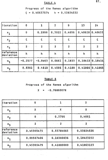
The b e s t a p p r o x i m a t i o n can be f ound by t h e second a l g o r i t h m o f Remes (RemeS/ 1 9 3 4 ) / a l s o c a l l e d t h e exch an ge a l g o r i t h m . A s e a r c h i s made f o r t h e p+1 p o i n t s o f
e x t r e m a l d e v i a t i o n o f t h e e r r o r f u n c t i o n r ( X / 0 t ) f o r t h e
'Kj
c u r r e n t a p p r o x i m a t i o n w h i c h a r e a l t e r n a t i v e l y + and
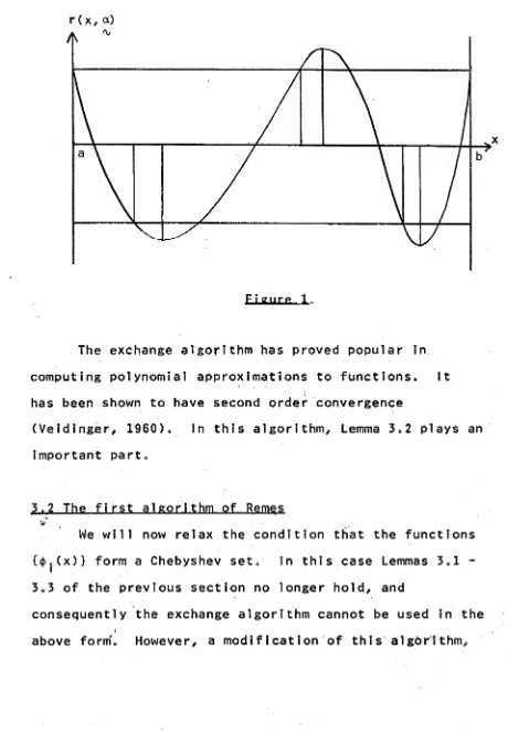
Thus/ t h e c u r r e n t s o l u t i o n f or ms a r e f e r e n c e v e c t o r w i t h r e s p e c t t o t h e s e p o i n t s as a r e f e r e n c e s e t . T h i s s h o u l d be made c l e a r by F i g u r e 1/ wh e r e t h e end p o i n t s a r e
p o i n t s o f t h e o r i g i n a l r e f e r e n c e / and r e ma i n as p o i n t s o f t h e new r e f e r e n c e . T h i s i s t h e u s u a l c a s e . A new
r (x, a)
figure 1 .
The exchange algorithm has proved popular in
computing polynomial approximations to functions. It
has been shown to have second order convergence
(Veidinger, I960). In this algorithm, Lemma 3.2 plays an
important part.
3.2 The first algorithm of Remes
We will now relax the condition that the functions
{4». (x ) } form a Chebyshev set. In this case Lemmas 3 01
-3.3 of the previous section no longer hold, and
consequently the exchange algorithm cannot be used in the
[image:48.551.70.530.63.725.2]c a l l e d t h e f i r s t a l g o r i t h m o f Remes ( Remes, 1 9 3 5 ) i s now a p p l i c a b l e » T h i s a l g o r i t h m , w h i c h was o r i g i n a l l y
d e v e l o p e d w i t h i n t h e f r a m e w o r k o f t h e c l a s s i c a l t h e o r y ( c f » t h e e x c h a n g e a l g o r i t h m o f S t i e f e l ) has been shown t o be a p p l i c a b l e i n t h e g e n e r a l ( n o n - c l ä s s i c a l ) c a s e by
Cheney ( 1 9 6 6 ) »
A s e q u e n c e o f c o r r e s p o n d i n g d i s c r e t e p r o b l e m s i s
t* h
c o n s i d e r e d « A t t h e r s t a g e , t h e d i s c r e t e p r o b l e m i s
(r)
Cr*)Cr)
s o l v e d on a s e t ( x . ) and a p p r o x i m a t i o n s h , a
j 'v
( r )
r e s u l t . The maxi mum o f | r ( x , a ) | on a $ x ( b i s now %
c a l c u l a t e d . L e t t h i s be a t t a i n e d a t a p o i n t £ r . Then we
( r + 1 ) )
s e t { x . } = ( x . ) U £ and r e p e a t t h e p r o c e d u r e «
J J r
( r ) I n Cheney ( 1 9 6 6 ) , i t i s shown t h a t t h e s e q u e n c e h
( r )
c o n v e r g e s . H o w e v e r , t h e a % w i l l n o t n e c e s s a r i l y c o n v e r g e u n l e s s t h e s o l u t i o n t o t h e c o n t i n u o u s p r o b l e m i s u n i q u e « A g e n e r a l i s a t i o n o f t h i s a l g o r i t h m f o r t h e n o n l i n e a r c a s e
i s g i v e n i n C h a p t e r 4, and c o n v e r g e n c e r e s u l t s s i m i l a r t o t h o s e o f C h e n e y ' s a r e p r o v e d .
Remar k 4 The f i r s t a l g o r i t h m o f Remes has been g e n e r a l i s e d by L a u r e n t ( 1 9 6 7 ) t o s o l v e t h e f o l l o w i n g p r o b 1em:
L e t E be a nor med v e c t o r s p a c e , and l e t V be a f i n i t e
*
![TABLE 8101 points in [l. 9507,3], p=l,q=2](https://thumb-us.123doks.com/thumbv2/123dok_us/1838610.140058/99.551.72.513.51.725/table-points-in-l-p-l-q.webp)