Regions: Statistical yearbook 2006: Data 2000 2004 2006 ed

(1)

THEME General and regional statistics

2006 EDITION

E U R O P E A N C O M M I S S I O N

Regions:

Statistical

yearbook 2006

Data 2000-2004

(2)

A great deal of additional information on the European Union is available on the Internet. It can be accessed through the Europa server (http://europa.eu).

Cataloguing data can be found at the end of this publication.

Luxembourg: Office for Official Publications of the European Communities, 2006 ISBN 92-79-01799-3

ISSN 1681-9306

Copyright for the following photos: cover and pages 9, 37, 65, 77, 119, 145: Jean-Jacques Patricola; cover and pages 13, 25, 51, 91, 105, 131: Regional Policy DG, European Commission.

For reproduction or use of these photos, permission must be sought directly from the copyright holder.

Printed in Belgium

http://ec.europa.eu/eurostat

Eurostat on the Internet

Our website is updated daily. Visit it today and get:

• direct and free access to all Eurostat PDF publications;

• direct and free access to our databases, presenting the latest and most complete statistical information available on the European Union, the EU Member States, the euro zone, the European Economic Area and other European partner countries;

• alert me — customisable e-mail alerts that inform you immediately when new data or publi-cations on your preferred topics become available;

• specialised access to short-term economic data;

• complete information on all Eurostat products and services.

European Statistical Data Support

Eurostat has set up with the members of the ‘European statistical system’ a network of support centres which will exist in nearly all Member States as well as in some EFTA countries. Their mission is to provide help and guidance to Internet users of European statistical data.

Contact details for this support network can be found on our Internet site.

Media Support Eurostat

Journalists can contact the media support service:

Tel. (352) 4301-33408 Fax (352) 4301-35349

E-mail: [email protected]

Europe Direct is a service to help you find answers to your questions about the European Union

Freephone number (*):

00 800 6 7 8 9 10 11

(*) Certain mobile telephone operators do not allow access to 00-800 numbers or these calls may be billed.

(3)

EUROSTAT

L-2920 Luxembourg — Tel. (352) 43 01-1 — http://ec.europa.eu/eurostat

Eurostat is the Statistical Office of the European Communities. Its task is to gather and analyse figures from the different European statistical offices in order to provide comparable and harmonised data for the European Union to use in the definition, implementation and analysis of Community policies. Its statistical products and services are also of great value to Europe’s business community, professional organisations, academics, librarians, NGOs, the media and citizens.

To ensure that the vast quantity of accessible data is made widely available and to help each user make proper use of the information, Eurostat has set up a publications and services programme.

This programme makes a clear distinction between general and specialist users and particular collections have been developed for these different groups. The collections Press releases,

Statistics in focus, Panorama of the European Union, Pocketbooks and Catalogues are aimed at general users. They give immediate key information through analyses, tables, graphs and maps.

The collections Detailed tables and Methods and nomenclatures suit the needs of the specialist who is prepared to spend more time analysing and using very detailed information and tables.

As part of the new dissemination policy, Eurostat has developed its website. All Eurostat publications are downloadable free of charge in PDF format from the website. Furthermore, Eurostat’s databases are freely available there, as are tables with the most frequently used and demanded short- and long-term indicators.

Eurostat has set up with the members of the ‘European statistical system’ a network of support centres which will exist in nearly all Member States as well as in some EFTA countries. Their mission is to provide help and guidance to Internet users of European statistical data. Contact details for this support network can be found on our Internet site.

Eurostat

(4)

ACKNOWLEDGEMENTS

The editing of each chapter of this publication would not have been possible without the participation of the following subject experts within the various Eurostat units:

• Population: Gregor Kyi (unit F1 Demographic and migration statistics)

• Regional gross domestic product: Andreas Krüger (unit C2 National accounts – production)

• Household accounts: Andreas Krüger (unit C2 National accounts – production)

• Regional labour market: Michal Mlady (unit D2 Regional indicators and geographical informa-tion)

• Labour productivity: Berthold Feldmann (unit D2 Regional indicators and geographical infor-mation)

• Urban statistics: Teodóra Brandmüller (unit D2 Regional indicators and geographical informa-tion)

• Science, technology and innovation: Bernard Felix, Simona Frank, August Götzfried and Håkan Wilén (unit F4 Education, science and culture statistics)

• Structural business statistics: Ulf Johansson (unit G1 Structural business statistics)

• Health: Sabine Gagel (unit F5 Health and food safety statistics)

• Transport: Caroline Heylen and Carla Sciullo (unit G5 Transport statistics)

• Agriculture: György Benoist and Michael Goll (E1 Agriculture statistics – methodology)

The process of creating this publication was coordinated by Åsa Önnerfors of unit D2 at Eurostat (Regional indicators and geographical information); Baudouin Quennery in unit D2 produced all the statistical maps, Michael Feith in unit B6 (Dissemination) helped us in the dissemination process.

We are also very grateful to:

Directorate General for Translation of the European Commission

(5)

p

INTRODUCTION

. . . 9

Statistical data at the regional level . . . 10

Some highlights . . . 10

Regional classification . . . 10

Coverage . . . 10

Structure . . . 10

More regional information needed? . . . 11

Regional interest group on the web . . . 11

Closure date for the yearbook data . . . 11

p

1. POPULATION

. . . 13

Introduction . . . 15

A changing population… . . . 15

… and a shifting age structure . . . 19

What will the future bring? . . . 20

Methodological notes . . . 22

p

2. REGIONAL GROSS DOMESTIC PRODUCT

. . . 25

What is regional gross domestic product? . . . 27

Regional GDP in 2003 . . . 27

Major regional differences even within the countries themselves . . . 29

Catching-up process in the new Member States is not successful everywhere . . . 31

Different trends even within the countries themselves . . . 33

Summary . . . 33

Purchasing power parities and international volume comparisons . . . 35

p

3. HOUSEHOLD ACCOUNTS

_{. . .} ₃₇

Introduction: Measuring wealth . . . 39

Private household income . . . 39

Results for 2003 . . . 39

Primary income and disposable income . . . 40

Income and social benefits . . . 43

Not all the new Member States are catching up . . . 45

Summary . . . 48

The measurement unit for regional comparisons . . . 49

p

4. REGIONAL LABOUR MARKET

. . . 51

Methodology . . . 53

Employment – the 15-64 age group . . . 54

Regions with high employment rates . . . 54

Regions with employment rates immediately below the highest level . . . 54

Regions with low employment rates . . . 56

Employment in Bulgaria and Romania . . . 57

Employment – the 55-64 age group . . . 58

High employment rates for persons aged 55 to 64 . . . 58

R e g i o n s : S t a t i s t i c a l y e a r b o o k 2 0 0 6 5

(6)

Low employment rates for persons aged 55 to 64 . . . 59

Employment rates for persons aged 55 to 64 in Bulgaria and Romania . . . 60

Unemployment . . . 60

Conclusion . . . 63

Definitions . . . 63

p

5. LABOUR PRODUCTIVITY

. . . 65

Marked differences in regional labour productivity . . . 67

Productivity growth rates: the new Member States are catching up . . . 70

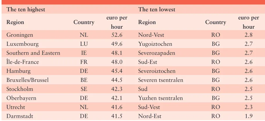
Labour productivity in terms of hours worked . . . 72

Conclusion . . . 74

p

6. URBAN STATISTICS

. . . 77

What is the Urban Audit? . . . 79

Spatial units . . . 79

Indicators . . . 79

Time . . . 80

Urban competitiveness . . . 81

Outputs . . . 81

Inputs . . . 83

Outcomes . . . 87

Outlook . . . 89

p

7. SCIENCE, TECHNOLOGY AND INNOVATION

. . . 91

Research and development . . . 93

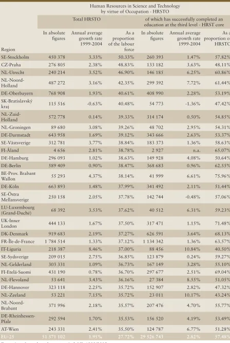
Human resources in science and technology . . . 96

Patents . . . 98

High-tech industries and knowledge-intensive services . . . 101

Conclusion . . . 101

Methodological notes . . . 103

p

8. STRUCTURAL BUSINESS STATISTICS

. . . 105

Lowest business diversification in small tourist regions and capital regions . . . 107

Retail trade the main activity in more than half the regions . . . 109

Many regions are highly specialised in a specific activity . . . 110

High-tech intensive regions relatively evenly distributed across the Member States . . . 110

Large differences in average wage costs among the high-tech intensive regions . . . 111

Highest investment rate in high-tech activities in Brussels . . . 114

p 9. HEALTH

. . . 119

Mortality in EU regions . . . 121

Ischaemic heart diseases . . . 122

(7)

Health Care resources in EU regions . . . 125

Hospital discharges . . . 125

Dentists . . . 127

p

10. TRANSPORT

. . . 131

Road network . . . 133

Vehicle stock . . . 135

Safety . . . 135

Maritime transport . . . 138

Aviation passengers . . . 140

p 11. AGRICULTURE

. . . 145

Methodological notes . . . 147

Structure of the agricultural holdings . . . 148

Environmental aspects . . . 152

Rural development statistics . . . 154

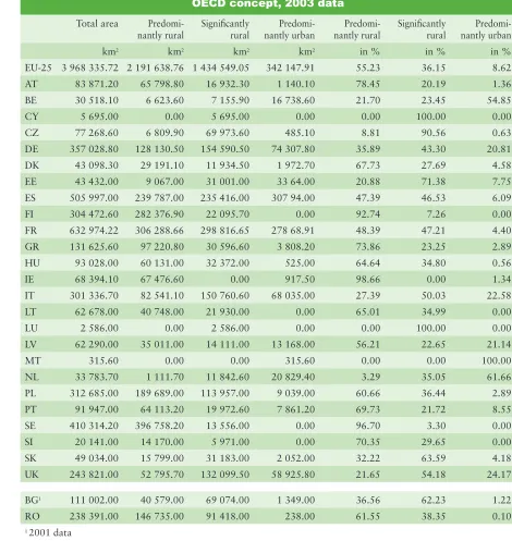
The OECD concept . . . 156

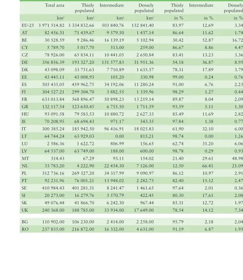
The Eurostat “degree of urbanisation” concept . . . 156

p

EUROPEAN UNION: NUTS 2 regions

. . . 163

p

CANDIDATE COUNTRIES: Statistical regions at level 2

. . . 165

(8)

(9)

Introduction

(10)

INTRODUCTION

Statistical data at the

regional level

The Structural Funds for the period 2007 to 2013 were decided in December 2005. This decision was based on the objective regional statistics compiled by Eurostat, thus highlighting the im-portance of our effort to produce a wide range of comparable regional information.

This yearbook shows many aspects of this region-al data and suggests in the various chapters some of the analyses which can be made with them. But we also invite you the reader to yourself continue the analyses of the regional data supplied in each of the different themes presented here. We also hope that this publication will make you keen to further investigate Eurostat’s statistical databases (available free of charge on the internet).

In keeping with the traditions of the Regional yearbook, we try to renew the publication a little each year, but also to keep its structure basically unchanged. In this way, many subjects reappear from year to year, but the theme or focus of the subject is always slightly different. This year we again have one theme that is totally new for the Regional Yearbook, namely “labour productiv-ity”, which combines statistics on GDP with labour market statistics in a very interesting way. This kind of cross-cutting of different statisti-cal domains could of course also be conducted with other statistical themes, but we will for the moment leave that to a future edition of the yearbook.

Some highlights

We will not present here the content of all chap-ters of this Regional Yearbook. Here, however, are some hints to whet your appetite to read it carefully:

• The population chapter this year focuses on old and young dependency ratios in the com-ing decades, highlightcom-ing the drastic changes of society we will have to cope with.

• The chapter on regional GDP centres its at-tention on growth rates between 1999 and 2003, giving interesting insights into regional differences.

• The Urban Audit chapter concentrates on the competitiveness of cities, analysing various facets of benchmarking cities that compete against each other.

• The chapter on the Structural Business Survey focuses on specialised regions in different in-dustrial and service activities. This highlights the heterogeneity of European regions in terms of the production process and skills.

Regional

classification

All regional analysis in this yearbook is based on NUTS 2003. In the meantime, the ten new Mem-ber States have also been formally integrated into the new regional classification in the form of an amendment to the NUTS Regulation. The texts of the Regulation and the amendment are avail-able on the CD-ROM – as is the annex, which lists the regions making up the nomenclature in each country.

Coverage

No distinction is made in the yearbook between the old Member States, the countries that became Member States in 2004 and those due to join in 2007 or 2008: wherever data are available for Bulgaria and Romania, these of course also feature in the maps and commentaries. In the case of Turkey and Croatia, there are still too few regional data to justify including them in the analyses.

Structure

(11)

R e g i o n s : S t a t i s t i c a l y e a r b o o k 2 0 0 6 1111 In order to assist the understanding of the maps,

the data series used for the maps in the yearbook are provided as Excel files on the CD-ROM.

In the maps, the statistics are presented at NUTS level 2. A map giving the code numbers of the regions can be found in the sleeve of this publi-cation. At the end of the publication there is a list of all the NUTS-2 regions in the European Union, together with a list of the level 2 sta-tistical regions in Bulgaria and Romania. Full details of these national regional breakdowns, including lists of level 2 and level 3 regions and the appropriate maps, may be consulted on the RAMON server.1

More regional

information needed?

The public REGIO database on the Eurostat web-site contains more extensive time series (which may go back as far as 1970) and more detailed statistics than those given in this yearbook, such as population, death and birth by single years of age, detailed results of the Community labour-force survey, etc. Moreover, there is coverage in REGIO of a number of indicators at NUTS level 3 (such as area, population, births and deaths, gross domestic product, unemployment rates). This is important because there are no fewer than eight EU Member States (Cyprus, Denmark, Estonia, Latvia, Lithuania, Luxembourg, Malta and Slov-enia) that do not have a level 2 breakdown.

For more detailed information on the contents of the REGIO database, please consult the Eurostat publication ‘European regional and urban statis-tics — Reference Guide 2003’, a copy of which is available in PDF format on the accompanying CD-ROM.

In addition, the reader is also invited to consult the web version of the “Portraits of the Regions”, which give regional profiles of all individual regions across Europe.2_{These regional topical}

profiles describe the geography and history of the region, before going on to assess its strengths and weaknesses in terms of demographic, economic and cultural issues. Among the aspects examined are the labour market, education, infrastructure and resources.

Regional interest

group on the web

Eurostat’s regional statistics team maintains a publicly accessible interest group on the web (‘CIRCA site’) with many useful links and docu-ments.3

Among other resources, you will find:

• a list of all regional coordination officers in the Member States, the candidate countries and the EFTA countries;

• the latest edition of the “Regional and Urban Reference Guide”;

• PowerPoint presentations of Eurostat’s work concerning regional and urban statistics;

• the regional classification NUTS for the Mem-ber States and the regional classification of the candidate countries.

Closure date for the

yearbook data

The cut-off date for this issue was the 15th_{of May}

2006.

1 _{See http://europa.eu.int/comm/eurostat/ramon/index.}

cfm?TargetUrl=DSP_PUB_WELC

2_See_{http://forum.europa.eu.int/irc/dsis/regportraits/info/}

data/en/index.htm

3 _See

http://forum.europa.eu.int/Public/irc/dsis/regstat/infor-mation

(12)

(13)

1.

Population

(14)

(15)

Introduction

Demographic trends have a strong impact on the societies of the European Union. Consistently low fertility levels, combined with an extended longevity and the fact that the baby boomers are reaching retirement age, result in a demographic ageing of the EU population. The share of the older generation is increasing while the share of those of working age is decreasing. If current trends prevail until 2050, a person of working age then might have to provide for up to twice as many retired people as is usual today.

The demographic development is not the same in all regions of the European Union. Although the ageing of their societies is a problem that all EU Member States have to face, it might have a stronger impact in some regions than in others. The regional pattern of major demographic phe-nomena, as it is visible today, is the focus of this chapter.

Some demographic developments might become considerably more important in the coming 50 years. To demonstrate the effects that current trends might have if continued in the future, Eurostat calculates population projections (see “Methodological notes”). The ‘Regions: Statisti-cal yearbook 2006’ presents projections of age dependency ratios in the EU-25 that give an idea of how much the current picture has to be seen in the context of time.

In its green paper “Confronting demographic change: a new solidarity between the genera-tions”1_{the European Commission concludes that}

in order to face up to demographic change, Eu-rope should pursue three essential priorities:

• Return to demographic growth.

• Ensure a balance between the generations, in the sharing of time throughout life, in the dis-tribution of the benefits of growth, and in that of funding needs stemming from pensions and health-related expenditure.

• Find new bridges between the stages of life, particularly between economic activity and inactivity. Young people still find it difficult to get into employment. An increasing number of “young retirees” want to participate in social and economic life. Study time is getting longer and young working people want to spend time with their children.

A changing

population…

During the last four decades, the population of the 25 countries of today’s European Union has grown from over 376 million persons (1960) to about 459 million persons (2005). How-ever, strength and composition of the popula-tion growth has varied significantly over the years. Until the end of the 1980s, the ‘natural increase’ (live births minus deaths) was by far the major component of population growth. However, there has been a sustained decline of the ‘natural increase’ since the early 1960s. On the other hand, international migration has gained importance to become the major force of population growth from the beginning of the 1990s onwards.

Maps 1.1, 1.2 and 1.3 show the total population change and its components since the start of the new century. For the sake of comparability, the

1 _{COM 2005, 94 fi nal.}

(16)

POPULA

TION

11

Map 1.1

AÇORES P

0 100

MADEIRA P

0 25

CANARIAS E

0 100

GUADELOUPE

F 0 25

MARTINIQUE

F 0 20

RÉUNION

F 0 20

GUYANE

F 0 100

0 100 500 km −0.4 − 0.0

−1.2 − −0.4 −2.8 − −1.2 −6.0 − −2.8 <= −6.0

> 12.0 5.6 − 12.0 2.4 − 5.6 0.8 − 2.4 0.0 − 0.8 Data not available

0 50

CYPRUS

0 10

MALTA

Total population change

Average for 2000 to 2003 − NUTS 2

Per 1000 inhabitants

UK: 2001

Statistical data: Eurostat − Database: REGIO © EuroGeographics, for the administrative boundaries Cartography: Eurostat − GISCO, 07/2006

population change is presented in relative terms, i.e. it is related to the size of the total population. The maps show the four year average for the re-sulting ‘crude rates of population change’ (for the years 2000, 2001, 2002 and 2003).

In the North-east of the European Union, the population is decreasing. Map 1.1 is marked by a clear divide between the regions there and in the rest of the EU. Most affected by a decreas-ing population are eastern Germany, Poland,

the Czech Republic, Slovakia and Hungary, and to the north the three Baltic States, and parts of Sweden and Finland.

(17)

AÇORES P

0 100

MADEIRA P

0 25

CANARIAS E

0 100

GUADELOUPE

F 0 25

MARTINIQUE

F 0 20

RÉUNION

F 0 20

GUYANE

F 0 100

0 100 500 km −0.4 − 0.0

−1.2 − −0.4 −2.8 − −1.2 −6.0 − −2.8 <= −6.0

0 50

CYPRUS

0 10

MALTA UK: 2001

Natural population change (Live births minus deaths)

Per 1 000 inhabitants

DE: 2003

FR (without DOMs): average of 2000, 2001, 2002 DOMs: average of 2000, 2001

Map 1.2

Map 1.2 shows that in many regions of the EU more persons have died than have been born since the start of the new century. The resulting negative ‘natural population change’ is wide-spread and the pattern is less pronounced as for the total population change. Ireland, France, the three Benelux countries and Denmark have mainly a ‘natural increase’ of the population. The ‘natural population change’ is predomi-nantly negative in Germany, the Czech

Repub-lic, Slovakia, Hungary, Slovenia and adjacent regions, as well as the Baltic States, Sweden in the north and Greece in the south. The other Member States have a situation that is, overall, more balanced.

A major reason for the slowdown of the ‘natu-ral increase’ of the population is the fact that, on average and over time, the inhabitants of the EU have fewer children. In the 25 countries that today form the European Union, the total

(18)

POPULA

TION

11

fertility rate has declined from a level of above 2.5 in the early 1960s to a level of about 1.5 in 1995 where it has remained since (graph 1.1; for the definition of the Total fertility rate in the “Methodological notes”). For comparison: In the more developed parts of the world today, a total fertility rate of around 2.1 children per women is considered to be the replacement level, i.e. the level at which a population would remain stable in the long run if there was no inward or outward migration.

Concerning net migration, four cross-border re-gions where more persons have left than arrived can be identified on map 1.3:

• The northern most regions of Sweden and Finland;

• A north-eastern group, comprising most of eastern Germany, Poland, Lithuania and Latvia as well as parts of the Czech Republic, Slovakia and Hungary;

• Regions in the north of France;

• Regions in the south of Italy.

In some regions a negative ‘natural change’ has been compensated by a positive net migration. This is most conspicuous in western Germany, eastern Austria, the north of Italy, and Slovenia, as well as the south of Sweden and regions in Spain, Greece and the United Kingdom. The

opposite is much rarer: in only a few regions (namely in the north of Poland), a positive ‘natu-ral change’ has been compensated by a negative net migration.

Regions without compensation are often ex-posed to a profound development, upwards or — in some regions — downwards. In Ireland, the Benelux countries, many regions in France and some in Spain a ‘natural increase’ has been accompanied by positive net migration. How-ever, in East Germany, Lithuania and Latvia, as well as some regions in Poland, the Czech Republic, Slovakia and Hungary both compo-nents of population change where negative. In some regions this has led to a sustained popula-tion loss.

An example: in the five Länder in eastern Ger-many2_{there were over half a million persons}

fewer on 1st_{January 2005 than on 1}st

Janu-ary 2000, reflecting a total population loss of 3.7 % of the population there. However, this movement is not homogeneous for all ages: The very young population (aged up to 14 years) decreased by almost a quarter (- 24.1 %) while the population at retirement age increased by 18.2 %.

2_{Berlin not included. Contrary to the rest of the analysis, this}

(19)

AÇORES P

0 100

MADEIRA P

0 25

CANARIAS E

0 100

GUADELOUPE

F 0 25

MARTINIQUE

F 0 20

RÉUNION

F 0 20

GUYANE

F 0 100

0 100 500 km −0.4 − 0.0

−1.2 − −0.4 −2.8 − −1.2 −6.0 − −2.8 <= −6.0

0 50

CYPRUS

0 10

MALTA UK: 2001

Net migration

Per 1 000 inhabitants

DE: 2003

FR (without DOMs): average of 2000, 2001, 2002 DOMs: average of 2000, 2001

Map 1.3

… and a shifting age

structure

Age dependency ratios are important demo-graphic indicators that relate the young and old age population to the population of working age. The ‘old age’ roughly approximates to the age of retirement. Today, different demographic reports

present dependency ratios based on different definitions for the age groups. In this publication the following age groups are being used:

• “Young age dependency ratio”: the tion aged up to 14 years related to the popula-tion aged between 15 and 64 years.

• “Old age dependency ratio”: the population aged 65 years or older related to the popula-tion aged between 15 and 64 years.

(20)

POPULA

TION

1

AÇORES P

0 100

MADEIRA P

0 25

CANARIAS E

0 100

GUADELOUPE

F 0 25

MARTINIQUE

F 0 20

RÉUNION

F 0 20

GUYANE

F 0 100

0 100 500 km > 28

26 − 28 24 − 26 22 − 24 <= 22

Data not available

0 50

CYPRUS

0 10

MALTA

2004 − NUTS 2

Young age dependency

Population ratio (in %)

by age: < 15 / 15−64

EL, FR, UK (excl. Scotland): 2003; Scotland: 2000. EU−25 = 24.4

Map 1.4

The maps 1.4 and 1.5 show the population struc-ture in the year 2004. The young age dependency ratio is influenced by recent fertility levels. Coun-tries with higher fertility tend to have a higher young age dependency (i.e. more young people per 100 of working age) when compared to coun-tries with low fertility levels. This is conspicuous for Ireland, France, the United Kingdom, the Benelux countries, Denmark, Sweden and Fin-land. The young age dependency is below average in regions in Italy, Greece, Spain, Germany, the

Czech Republic and Latvia. The regional pattern for the old age dependency is less clear cut.

What will the future

bring?

(21)

AÇORES P

0 100

MADEIRA P

0 25

CANARIAS E

0 100

GUADELOUPE

F 0 25

MARTINIQUE

F 0 20

RÉUNION

F 0 20

GUYANE

F 0 100

0 100 500 km > 29

26 − 29 23 − 26 20 − 23 <= 20

Data not available

0 50

CYPRUS

0 10

MALTA

2004 − NUTS 2

Old age dependency

Population ratio (in %)

by age: > 64 / 15−64

EL, FR, UK (excl. Scotland): 2003; Scotland: 2000. EU−25 = 24.5

Map 1.5

develop if current trends continue. A particularly dynamic indicator will probably be the old age dependency ratio. It is a reasonable projection that, on average for the EU-25 and if current trends prevail, the old age dependency ratio will approximately double during the next 50 years (graph 1.2). This means that in the year 2050 a person of working age might have to provide for up to twice as many retired people as is usual today. The regional differences visible already

today might lead to a more dramatic development in some regions than in others.

The example of the five Länder in eastern Ger-many demonstrates that in some regions the demographic ageing of the population is already developing quite fast. In this region, the young age dependency ratio has fallen from 19.4 % (2000) to 15.4 % (2005), whereas the old age dependency ratio has risen from 23.5 % (2000) to 29.2 % (2005).

(22)

1

!

!"

#$!%&'()%$* +& ($$!%&'()%$,+&

Methodological notes

Sources: Eurostat - Demographic Statistics. For more infor-mation please consult the Eurostat website at http://www. europa.eu.int/comm/eurostat/

The Total fertility rate is defined as the average number of children that would be born to a woman during her lifetime if she were to pass through her childbearing years conforming to the age specific fertility rates that have been measured in a given year. In the more developed parts of the world today, a total fertility rate of around 2.1 children per women is considered to be the replacement level, i.e. the level at which a population would remain stable in the long run if there was no inward or outward migration.

The Eurostat population projections presented here cor-respond to the baseline variant of the Trend scenario. The Eurostat set of population projections is just one among several scenarios of population evolution based on assumptions of fertility, mortality and migration. The current Trend scenario does not take into account any fu-ture measures that could influence demographic trends. It comprises different variants: the ‘baseline’ variant as well

as ‘high population’, ‘low population’, ‘zero-migration’, ‘high fertility’, ‘younger age profile’ and ‘older age profile’ variants, all available on the Eurostat website. It should be noted that the assumptions adopted by Eurostat may dif-fer from those adopted by National Statistical Institutes. Therefore, results can be different from those published by Member States.

Migration can be extremely difficult to measure. A variety of different data sources and definitions are used in the Member States, meaning that direct comparisons between national statistics can be difficult or misleading. The net migration figures here are not directly calculated from immigration and emigration flow figures. As many EU Member States do not have complete and comparable fig-ures for immigration and emigration flows, net migration is estimated here as the difference between the total popu-lation change and the ‘natural increase’ over the year. In effect, net migration equals all changes in total population that cannot be attributed to births and deaths.

The population density is the ratio of the mid-year population of a territory on a given date to the size of the territory.

POPULA

(23)

R e g i o n s : S t a t i s t i c a l y e a r b o o k 2 0 0 6 23 Map 1.6

AÇORES P

0 100

MADEIRA P

0 25

CANARIAS E

0 100

GUADELOUPE

F 0 25

MARTINIQUE

F 0 20

RÉUNION

F 0 20

GUYANE

F 0 100

0 100 500 km > 520

260 − 520 130 − 260 65 − 130 <= 65

Data not available

0 50

CYPRUS

0 10

MALTA

2003 − NUTS 2

EU−25 = 117

Population density

Inhabitants per km²

Scotland and Northern Ireland: 2002

(24)

(25)

2.

Regional gross

domestic

product

(26)

(27)

What is regional

gross domestic

product?

The economic development of a region is, as a rule, expressed in terms of its gross domestic product (GDP). This is also an indicator fre-quently used as a basis for comparisons between regions. But what exactly does it mean? And how can comparability be established between regions of different sizes and with different currencies?

Regions of different sizes achieve different levels of GDP. However, a real comparison can only be made by comparing the regional GDP with the population of the region in question. This is where the distinction between place of work and place of residence becomes significant: GDP measures the economic performance achieved within national or regional boundaries, regard-less of whether this was attributable to resident or non-resident employed persons. Reference to GDP per inhabitant is therefore only straight-forward if all employed persons engaged in generating GDP are also residents of the region in question.

In areas with a high proportion of commuters, regional GDP per inhabitant can be extremely high, particularly in economic centres such as London or Vienna, Hamburg, Prague or Lux-embourg, and relatively low in the surrounding regions, even if primary household income in these regions is very high. Regional GDP per inhabitant should therefore not be equated with regional primary income.

Regional GDP is calculated in the currency of the country in question. In order to make GDP

comparable between countries, it is converted into euros using the official average exchange rate for the given calendar year. However, ex-change rates do not reflect all the differences in price levels between countries. In order to equate the currencies, GDP is converted using currency conversion rates, known as Purchasing Power Parities (PPPs), into an artificial common currency, called the Purchasing Power Standard (PPS). This makes it possible to compare the purchasing power of the different national cur-rencies (see box).

Regional GDP in

2003

Map 2.1 gives an overview of the regional distri-bution of per capita GDP (in PPS) for the Europe-an Union, plus Bulgaria Europe-and RomEurope-ania. It rEurope-anges from PPS 4 721 per capita in north-east Romania to PPS 60 342 per capita in the UK capital re-gion of Inner London. Brussels (PPS 51 658) and Luxembourg (PPS 50 844) follow in second and third places, with Hamburg (PPS 40 011) and the French capital region Île-de-France (PPS 37 687) in fourth and fifth places.

Prague (Czech Republic), the region with the highest GDP per inhabitant in the new Member States with PPS 30 052 (138% of the EU-25 average), has already risen to nineteenth place (2002: 20th) among the 268 NUTS 2 regions of the countries examined here (EU-25 plus Bulgaria and Romania). It should be noted, however, that Prague is an exception among the regions of the new Member States. The next regions of those which joined the EU in 2004 and of the candidate countries follow some

(28)

REGIONAL GROSS DOMESTIC PRODUCT

2

way behind: Bratislavský kraj (Slovakia) is only in 53rd place (2002: also 53rd) with PPS 25 190 (116%), Közép-Magyarország (Hungary) is 130th (2002: also 130th) with PPS 20 627 (95%), Cyprus is 180th (2002: 170th) with PPS 17 377 (80%), Slovenia is 190th (2002: 191st) with PPS 16 527 (76%), Mazowieckie (Poland) is 203rd (2002: 204th) with PPS 15 833 (73%) and Malta is 204th (2002: 194th) with PPS 15 797 (73%). All other regions in the new Member

States and candidate countries have a per capita GDP in PPS of less than two-thirds of the EU-25 average.

In 74 of the 268 regions examined here, the per capita GDP (in PPS) in 2003 was less than 75% of the EU-25 average. As can be seen from Map 2.2, most of these regions are in the southern and western periphery of the EU, as well as in eastern Germany, the new Member States and the

candi-AÇORES P

0 100

MADEIRA P

0 25

CANARIAS E

0 100

GUADELOUPE

F 0 25

MARTINIQUE

F 0 20

RÉUNION

F 0 20

GUYANE

F 0 100

0 100 500 km > 26 000

20 000 −26 000 14 000 −20 000 8 000 −14 000 <= 8 000 Data not available

0 50

CYPRUS

0 10

MALTA

2003 − NUTS 2

EU−25 = 21 741

GDP per inhabitant, in PPS

(29)

R e g i o n s : S t a t i s t i c a l y e a r b o o k 2 0 0 6 29 date countries. This group has been considerably

reduced in size since 2002, when it comprised 80 regions. In Spain and Greece in particular, two regions in each country crossed the 75% of per capita GDP barrier.

At the upper end of the spectrum, 36 regions had a per capita GDP of more than 125% of the EU-25 average in 2003, down from 41 in 2002. Most of these particularly affluent regions are in southern Germany, in the south of the UK, in northern Italy and in Belgium, Luxembourg, the Netherlands, Ireland and Scandinavia. Madrid, Prague and Paris also fall into this category.

The central part of the distribution curve, which includes the regions with a per capita GDP of between 75% and 125% of the EU-25 average, thus increased from 147 regions in 2002 to 158 regions in 2003. Economic convergence between the regions of the 27 countries examined here therefore clearly improved in 2003: the range of per capita GDP values between Inner

Lon-don and north-east Romania fell from 13.9:1 in 2002 to 12.8:1 in 2003. The least affluent regions also benefited from this development, with the number of regions with GDP values below 40% of the EU average falling from 23 in 2002 to 21 in 2003.

Major regional

differences even

within the countries

themselves

There are also substantial regional differences even within the countries themselves, as Graph 2.1 shows. In 2003, the highest per capita GDP value was more than double the lowest value in 12 of the 19 countries examined here, which

ph 2.1: GDP per inhabitant (in PPS) 2003, NUTS 2, in percent of EU-25 average (EU-25=100)

Bruxelles Hainaut BE CZ DK DE EE EL ES FR IE IT LV LT HU NL AT PL PT FI RO SE UK SK 25

0 50 75 100 125 150 175 200

Praha Moravskoslezsko Dessau Sterea Ellada Anatoliki Makedonia, Thraki Madrid Extremadura Île-de-France Guyane

Southern and Eastern Border, Midland and Western

Bolzano Calabria Közép-Magyarország Észak-Magyarország Utrecht Flevoland Wien Burgenland Mazowieckie Lisboa Norte Hamburg Lubelskie 225 250 LU MT SI BG CY V chodné

Slovensko _{Bratislavsk kraj} Itä-Suomi Åland Östra Mellansverige Stockholm

West Wales and The Valleys Inner London

275 300

Severen

Tsentralen Yugozapaden Nord-Est

Average of all areas of the country Capital city area of the country Bucuresti

(30)

REGIONAL GROSS DOMESTIC PRODUCT

2

include several NUTS 2 regions (2002: also 12). This group includes 5 of the 6 new Member States/candidate countries but only 7 of the 13 EU-15 Member States.

The largest regional differences are in the United Kingdom and Belgium, where there is a factor of 3.7 and 3.1 respectively between the two extreme values. The lowest values are in Ireland and Swe-den, with a corresponding factor of 1.6 in each

case. Moderate regional disparities in per capita GDP (i.e. factors of less than 2 between the high-est and the lowhigh-est value) are found only in the EU-15 Member States and Bulgaria.

Comparatively large regional disparities in per capita GDP are therefore still evident not only in the EU-15 countries but also in the new Member States and candidate countries. However, there was a slight narrowing of the range of values

AÇORES P

0 100

MADEIRA P

0 25

CANARIAS E

0 100

GUADELOUPE

F 0 25

MARTINIQUE

F 0 20

RÉUNION

F 0 20

GUYANE

F 0 100

0 100 500 km

> 125 % 100 − 125 % 81.8 − 100 % 75 − 81.8 % < 75 %

0 50

CYPRUS

0 10

MALTA

2003 − NUTS 2

GDP per inhabitant (in PPS),

in % of EU25 = 100

(31)

R e g i o n s : S t a t i s t i c a l y e a r b o o k 2 0 0 6 31 in both groups of countries between 2002 and

2003. Regional convergence can therefore be seen not only vis-à-vis the EU average but also within most countries.

In all the new Member States and candidate countries, and in a number of the EU-15 Member States, a substantial share of economic activity is concentrated in the capital regions. In 13 of the 19 countries included here in which there are several NUTS 2 regions, the capital regions are also the regions with the highest per capita GDP. For example, Maps 2.1 and 2.2 clearly show the prominent position of the regions of Brussels, Prague, Madrid, Paris, Lisbon as well as Buda-pest, Bratislava, London, Sofia and Bucharest.

Catching-up process

in the new Member

States is not

successful everywhere

Map 2.3 shows the extent to which per capita GDP changed between 1999 and 2003 by com-parison with the EU-25 average (expressed in percentage points of the EU-25 average). Eco-nomically dynamic regions, whose per capita GDP increased by more than one percentage point compared to the EU average, are shown in green. Less dynamic regions (those with a fall of more than one percentage point in per capita GDP compared to the EU-25 average) are shown in orange and red. The values range from +18.1 percentage points for Groningen (Netherlands) to -11.7 percentage points for Trento in Italy.

The map shows that economic dynamism is well above average in the peripheral areas of the EU, not only in the EU-15 countries but also in the new Member States and accession countries. Among the EU-15 Member States, strong growth can be seen in Greece, Spain, Ireland and the United Kingdom, in particular. On the other hand, a trend revealed by earlier data has contin-ued, with persistent low growth in a few key re-gions of the EU founding Member States, and in Portugal. Italy, where not a single region achieved the average growth of the EU-25 between 1999 and 2003, and Portugal, where only Madeira was able to make progress vis-à-vis the EU-25, were

hit particularly hard by this unwelcome develop-ment. Most of the regions in Germany and France also fell short of the EU average.

Of the new Member States and the accession countries, where the capital regions are very dynamic, the Baltic countries, Hungary and Slov-enia, in particular, have experienced above-aver-age growth. Recent developments in Bulgaria and Romania are also encouraging, with only one region in each country falling below the EU-25 average. However, the increases in GDP values in Poland since 1999 have been only slightly above the EU-25 average, which is disappointing in view of the low level of GDP overall.

On closer analysis, it is immediately apparent that 12 regions increased by at least 10 percent-age points compared to the EU averpercent-age, while only eight fell by at least 10 percentage points. Of the regions which are particularly dynamic, three are in Greece, two in the United King-dom and four in the new Member States/acces-sion countries. The fastest growing regions are therefore scattered relatively widely across the countries examined here. However, eight of these 12 regions are capital regions, which continue to have an above-average rate of growth not only in the EU-15 countries but also in the new Member States and accession countries.

The EU-15 countries which have particularly poor growth are concentrated at the lower end of the distribution curve. Of the eight regions which fell by more than 10 percentage points in com-parison with the EU average, four are in Italy, three in Germany and one in Portugal.

A more diverse picture emerges by including re-gions which either gained or lost at least five per-centage points against the EU average between 1999 and 2003.

It can be seen from the upper end of the distribu-tion curve that the 56 most successful regions include 11 out of 13 regions in Greece. These are joined by 16 out of 37 regions in the UK and nine out of 19 regions in Spain. This means that 36 of the 56 most successful regions are located in these three countries. In total, 43 regions from this group are in the EU-15 countries.

This shows that 13 regions in the new Member States and accession countries have gained at least 5 percentage points compared to the EU average. The capital regions in Romania and Hungary (both + 16.2 percentage points),

(32)

REGIONAL GROSS DOMESTIC PRODUCT

2

kia (+ 13.9) and the Czech Republic (+ 10.9) were particularly successful. The non-capital region with the strongest growth among the regions in the new Member States and accession countries was Nord-Est in Romania, the per capita GDP (in PPS) of which increased by 6.7 percentage points between 1999 and 2003 from 22.4% to 29.1% of the EU-25 average.

A clear concentration of regions is also appar-ent at the lower end of the distribution curve: of

the 42 regions which fell by at least 5 percentage points, 20 are in Germany, ten in Italy, five in France and three in Portugal. A large number of German and Italian regions in this group have an above-average level of GDP, thus making the dis-appointing trend of recent years less unsatisfac-tory than in Portugal. The Portuguese regions of Norte (-8.2 percentage points) and Centro (-6.4), which had a GDP of less than 70% of the EU-25 average at the end of the 1990s, have fallen

AÇORES P

0 100

MADEIRA P

0 25

CANARIAS E

0 100

GUADELOUPE

F 0 25

MARTINIQUE

F 0 20

RÉUNION

F 0 20

GUYANE

F 0 100

0 100 500 km > + 5

+ 1 − + 5 − 1 − + 1 − 5 − − 1 <= − 5 Data not available

0 50

CYPRUS

0 10

MALTA

EU−25 = 0

Change of GDP per inhabitant (in PPS)

in percentage points of the average EU−25

2003 as compared with 1999 − NUTS 2

(33)

R e g i o n s : S t a t i s t i c a l y e a r b o o k 2 0 0 6 33 further behind to a worrying degree. This makes

the region of Norte the least prosperous region in the EU-15; in 2003, its GDP was 57.4% of the EU average, i.e. the same as that of the Romanian capital, Bucharest.

The new Member States and accession countries are catching up with the EU-25 average at a rate of 0.8 percentage points every year, which at first glance appears to be encouraging. On closer inspection, however, it is clear that not all coun-tries and regions were able to benefit from this: in particular, Poland, Cyprus and Malta, and, to some extent, the Czech Republic and Bulgaria. 24 of the 55 regions in the new Member States and accession countries gained fewer than three percentage points, which was below the aver-age; of those 24 regions, 12 are in Poland, six in the Czech Republic and three in Bulgaria. Eight regions fell even further behind: four in Poland, one in Bulgaria and one in Romania. The strong-est downturns were seen in Malta, with a drop of – 4.1 percentage points.

Different trends even

within the countries

themselves

Graph 2.2 illustrates the economic development of individual countries between 1999 and 2003. It shows that the dynamics of economic develop-ment between the regions in one country can diverge almost as widely as between regions in different countries. The greatest differences in dynamics can be seen in the Netherlands and Romania, where the per capita GDP in each of the most economically dynamic regions increased by around 20 percentage points more than in the least economically developed regions. The corresponding figures for the United Kingdom and Portugal were 17 and 15 percentage points respectively. At the opposite end of the scale lie Sweden and Belgium, with a regional range of 8 percentage points, and Poland, with a corre-sponding value of 3.6 percentage points.

The pronounced regional differences within the new Member States and accession countries can be attributed largely to the dynamic growth of the capital regions. However, there is no reason to believe, on the basis of the data available, that

major differences in the distribution of growth rates are typical of the new Member States or ac-cession countries.

Graph 2.2 also shows that the least economically dynamic regions in only a small number of coun-tries attained levels of growth at least equal to the EU-25 average. This was achieved by only five of the 19 countries with several NUTS 2 regions examined here: the Czech Republic, Greece, Ire-land, Hungary and Slovakia.

Summary

In 2003, the highest and lowest values of per capita GDP (in PPS) for the 268 regions examined here differed in 27 countries by a factor of 12.8 : 1, which is still very high but slightly lower than the previous year. The number of regions with per capita GDP (in PPS) below 75% of the EU-25 average also fell from 80 to 74. Economic con-vergence between the regions therefore improved in 2003.

Economic development in the EU-15 countries was characterised by dynamic growth in Greece, the UK and Spain. This contrasted with disap-pointing economic development in most of the Italian, German and Portuguese regions. In the new Member States and accession countries, economic development in the Baltic countries and in Hungary, Romania and Bulgaria was particu-larly encouraging, while growth in most of the Polish regions remained disappointing.

Between 1999 and 2003, per capita GDP in-creased by more than five percentage points com-pared to the EU average in 56 regions. One or two regions in most countries fell behind, and in some cases far behind, in comparison with the EU average. The dynamics of growth in the capital regions of most countries was clearly above-aver-age. At the lower end of the scale were 42 regions which fell by at least five percentage points; most of them were in Germany, Italy and Portugal. As a result of the unsatisfactory economic de-velopment in Portugal, the regions of Norte and Centro, where GDP was already below 70% of the EU-25 average, fell again by around 8 and 6 percentage points respectively.

The new Member States and accession countries continued to catch up with the EU-25 average at a rate of around 0.8 percentage points every year.

(34)

REGIONAL GROSS DOMESTIC PRODUCT

2

However, not all the regions of the new Mem-ber States are able to benefit from this to the same extent. This is particularly true of Poland, Cyprus and Malta. All the new Member States taken together rose by 3.2 percentage points to 52.9% of the EU-25 average between 1999 and 2003. The corresponding values for Bul-garia and Romania were 3.7 and 4.7 percentage

points respectively. One region in each of these two accession countries was unable to share in this generally favourable economic develop-ment: Yugoiztochen in Bulgaria and Nord-Est in Romania. With per capita GDP standing at just under 22% of the EU-25 average, this region is the least affluent in the 27 countries examined here.

ph 2.2: Change of GDP per inhabitant (in PPS) in percentage points of the average EU-25, 2003 as compared with 1999 - NUTS 2

Average of all areas of the country Capital city area of the country

Brabant Wallon Liège BE CZ DK DE EE EL ES FR IE IT CY LV LT LU HU MT NL AT PL PT SI SK FI SE UK BG RO -10

-15 -5 0 5 10 15 25

Severozápad

Berlin

Notio Aigaio Illes Balears

Alsace

Border, Midland and Western Trento Dél-Alföld Utrecht Salzburg Zachodniopomorskie Lisboa Vychodné Slovensko Etelä-Suomi Stockholm

Highlands and Islands Yugoiztochen Nord-Est Praha Dresden Sterea Ellada Navarra Provence-Alpes-Côte d'Azur

Southern and Eastern Sicilia Közép-Magyarország Groningen Burgenland S´la˛skie Madeira

(35)

35

R e g i o n s : S t a t i s t i c a l y e a r b o o k 2 0 0 6

Purchasing power parities and

international volume comparisons

International differences in GDP values, even after con-version via exchange rates to a common currency, cannot be attributed solely to differing volumes of goods and services. The “level of prices” component is also a major contributing factor. Given that exchange rates are deter-mined by many factors influencing demand and supply in the currency markets (such as international trade, infla-tion expectainfla-tions and interest rate differentials), conver-sion via exchange rates in cross-border comparisons is of limited use. To obtain a more accurate comparison, it is essential to use special conversion rates (spatial deflators) which remove the effect of price-level differences between countries. Purchasing Power Parities (PPPs) are currency conversion rates of this kind which convert economic data expressed in national currencies into an artificial common currency, called Purchasing Power Standards (PPS). PPPs are therefore used to convert the GDP and other economic aggregates (e.g. consumption expenditure on certain prod-uct groups) of various countries into comparable volumes of expenditure, expressed in Purchasing Power Standards.

With the introduction of the euro, prices can now, for the first time, be compared directly between countries in the euro-zone. However, the euro has different purchasing power in the different countries of the euro-zone, depend-ing on the national price level. PPPs must therefore also continue to be used to calculate pure volume aggregates in PPS for Member States within the euro-zone.

In their simplest form, PPPs are a set of price relatives, which show the ratio of the prices in national currency of the same good or service in different countries (e.g. a loaf of bread costs €1.87 in France, €1.68 in Germany, £0.95 in the UK, etc.). A basket of comparable goods and services is

used for price surveys. These are selected so as to represent the whole range of goods and services, taking account of the consumption structures in the various countries. The simple price ratios at product level are aggregated to PPPs for product groups, then for overall consumption and finally for GDP. In order to have a reference value for the calculation of the PPPs, a country is usually chosen and used as the reference country, and set to 1. For the Euro-pean Union, the selection of a single country as the refer-ence country is inappropriate, so the PPS of the EU is used as an artificial common unit of reference to express the volume of economic aggregates for the purpose of spatial comparisons in real terms.

Unfortunately, for reasons of cost, it will not be possible in the foreseeable future to calculate regional currency conversion rates. If such regional PPPs were available, the GDP in PPS for numerous peripheral or rural regions of the EU would probably be higher than that calculated using the national PPPs.

The regions may be ranked differently when calculating in PPS instead of euros. For example, in 2003 the German region of Dessau was reported as having a per capita GDP of€17 145, putting it well ahead of Malta with €10 773. However, with PPS 15 797 per capita, Malta ranks above Dessau with its PPS 15 413 per capita.

In terms of distribution, the use of PPS rather than the euro has a levelling effect, as regions with a very high per capita GDP also generally have relatively high price levels. This reduces the range of per capita GDP in NUTS 2 regions in EU-25 plus Bulgaria and Romania from around €62 300 to around PPS 55 600.

Per capita GDP in PPS is the key variable for determining the eligibility of NUTS 2 regions under the European Un-ion’s structural policy.

(36)

(37)

Household

accounts

3.

(38)

(39)

Introduction:

Measuring wealth

One of the primary aims of regional statistics is to measure regions’ wealth. This is of particular relevance as a basis for policy measures which aim to provide support for less well-off regions.

The indicator most frequently used to measure re-gions’ wealth is regional gross domestic product (GDP). GDP is usually expressed in purchasing power standards (PPS) and per capita to make the data comparable between regions.

However, per capita regional GDP has a number of drawbacks as an indicator of wealth, one of which is that a “place-of-work” figure (the GDP produced in the region) is divided by a “place-of-residence” figure (the population living in the re-gion). This inconsistency is of relevance wherever there are commuter flows — i.e. more or fewer people working in a region than living in it. The most obvious example is the “Inner London” region of the UK, which has by far the highest per capita GDP. Yet this by no means translates into a correspondingly high income level for the inhabitants of the same region, as thousands of commuters travel to London every day to work there but live in the neighbouring regions. Ham-burg, Vienna, Luxembourg and Prague are other examples of this phenomenon.

Apart from the commuter flows, other factors can also cause the regional distribution of actual wealth not to correspond to GDP distribution. These in-clude, for example, income from rent, interest or dividends received by the residents of a certain region, but paid by residents of other regions. It is therefore useful to compare the regional GDP with the regional distribution of household income.

Private household

income

In market economies with State redistribution mechanisms, a distinction is made between two types of private-household income distribution.

The primary distribution of income reflects the

income of private households generated directly from market transactions, i.e. the purchase and sale of the factors of production and goods. These include in particular the compensation of employees. Private households can also receive income on assets, e.g. in the form of interest or rent. Finally, there is also income in the form of an operating surplus or self-employment income. Any interest or rent payable by the households is recorded as a negative item. The balance of all these transactions is termed the primary income

of private households.

The primary income is the point of departure for the secondary distribution of income, which denotes the State redistribution mechanism. All monetary social benefits and transfers received by the households are now added to primary income. On the other hand, households must use their income to pay taxes on income and wealth, pay their social contributions and effect trans-fers. The sum remaining after these transactions have been carried out, i.e. the balance, is called

the disposable income of private households.

Results for 2003

It is only in recent years that Eurostat has had data for these income categories of private

(40)

3 HOUSEHOL

D

A

C

O

UN

T

S

households. The data are collected in the re-gional accounts for NUTS level 2. Until recently, derogations still applied to several Member States, allowing their data to be submitted to Eurostat later than the 24 months after the end of the reference year stipulated in the Regula-tion or not at all; other Member States have not always kept to the deadline laid down in the Regulation.

There are still no data available for the follow-ing regions at NUTS 2 regional level: the French Overseas Departments, the Autonomous Prov-ince of Bolzano and the Autonomous ProvProv-ince of Trento in Italy, Cyprus, Luxembourg, Malta, Slovenia and Bulgaria. Values for EU-25 in this part of the regional accounts consequently re-main unavailable. This chapter therefore relates to the other 21 Member States and Romania.

Primary income and

disposable income

Map 3.1 gives an overview of primary income in the NUTS 2 regions of the 22 countries examined here. Centres of wealth in south-ern England, Paris and Alsace, northsouth-ern Italy, Vienna, Madrid, the País Vasco and Comuni-dad Foral de Navarra in Spain, Flanders, the western Netherlands, Stockholm and Nord-rhein-Westfalen, Hessen, Baden-Württemberg and Bayern in Germany are clearly evident. There is also a clear north-south divide in Italy and a west-east divide in Germany, while the regional distribution is relatively homogeneous in France. A south-north divide is evident in the UK, although to a lesser extent than in Italy and Germany.

In the new Member States, however, household primary income lies considerably below the EU average. The regions with clearly above-average levels of wealth are mainly capital regions, in particular Prague, Közép-Magyarország (Hun-gary), Mazowieckie (Poland) and Bucharest (Romania). Furthermore, the eastern peripheral regions of some of the new Member States are clearly even further behind the respective na-tional level.

The regional values range from 2 495 PPCS per capita in Nord-Est in Romania to 27 818 PPCS in the UK region of Inner London. The ten regions

with the highest per capita income include five regions in the UK alone, two each in Belgium and Germany and one in France.

A comparison of primary income with dispos-able income (map 3.2) shows the levelling influ-ence of State intervention. It visibly increases the relative income level in southern Italy, central and southern Spain, Galicia, the west and north of the UK and in parts of eastern Germany and central Greece. State activity moves several re-gions in northern and western Germany up to the same class as the affluent south-west of the country.

Similar effects can be observed in the new Mem-ber States, particularly in Hungary, Slovakia and most of the Polish regions. However, the levelling out of private income levels in the new Member States has generally been less pronounced than in EU-15.

In spite of State redistribution, most capital re-gions maintain their prominent position with the highest disposable income for the country in question.

The regional values range from 2 547 PPCS per capita in Nord-Est in Romania to 21 659 PPCS in the UK region of Inner London. Of the ten regions with the highest per capita disposable income, six are in the UK, two in Italy, one in France and one in Austria. The two Italian re-gions of Emilia-Romagna and Lombardia have moved into the group of the first ten regions, while the two German regions of Stuttgart and Oberbayern have moved out — a reflection of the fact that the levelling effect of State interven-tion on private income is much less pronounced in Italy than in Germany. At 11 214 PPCS per capita, Prague continues to be the region with the highest disposable income in the new Mem-ber States.

(41)

R e g i o n s : S t a t i s t i c a l y e a r b o o k 2 0 0 6 41 Italy is the only EU-15 Member State among the

five countries with the highest income dispari-ties, which include Hungary, the Czech Republic and Slovakia; in all four countries, the highest regional values exceed the lowest by approxi-mately 75%. Poland has the lowest income dis-parity of the new Member States (64%), which is close to that of Spain, Greece and Portugal. With values of between 53% and 41%, the re-gional disparities in the UK, France, Germany,

Belgium and Finland are relatively similar. The smallest regional income disparities are to be found in Ireland, Austria, the Netherlands and Sweden, where the maximum values exceed the minimum values by between 11% and 32%.

Graph 3.1 also shows that the capital cities of 11 of the 18 countries with several NUTS 2 re-gions also have the highest income values. This group includes all the larger new Member States and Romania. The economic dominance of the

AÇORES P

0 100

MADEIRA P

0 25

CANARIAS E

0 100

GUADELOUPE

F 0 25

MARTINIQUE

F 0 20

RÉUNION

F 0 20

GUYANE

F 0 100

0 100 500 km > 18 000

12 000 − 18 000 6 000 − 12 000 <= 6 000

Data not available

0 50

CYPRUS

0 10

MALTA

2003 − NUTS 2

IE: 2002

Primary income of private households per inhabitant, in PPCS

AT: Eurostat estimates

Map 3.1

(42)

3 HOUSEHOL

D

A

C

O

UN

T

S

capital regions is also evident when their income values are compared with the national averages. In three countries (Romania, the Czech Repub-lic and Slovakia), the capital cities exceed the national values by more than 50%. In only two countries (Belgium and Germany) are the values lower than the national averages.

Map 3.3 illustrates the relationship between disposable and primary income. This quotient gives an idea of the effects of State activity and

of other transfer payments. Substantial dif-ferences between the regions of the Member States are evident. Disposable income in the capital cities and other prosperous regions of EU-15 is almost without exception below 80% of primary income. Correspondingly higher percentages can be observed in the less affluent areas, in particular on the southern periphery of the EU, in the west of the UK and in eastern Germany.

AÇORES P

0 100

MADEIRA P

0 25

CANARIAS E

0 100

GUADELOUPE

F 0 25

MARTINIQUE

F 0 20

RÉUNION

F 0 20

GUYANE

F 0 100

0 100 500 km > 15 000

1 0000 − 15 000 5 000 − 1 0000 <= 5 000

Data not available

0 50

CYPRUS

0 10

MALTA

2003 − NUTS 2

IE: 2002

Disposable income of private households per inhabitant, in PPCS

AT: Eurostat estimates

Regions: Statistical yearbook 2006: Data 2000 2004 2006 ed

Regions:

Statistical

yearbook 2006

Data 2000-2004

http://ec.europa.eu/eurostat

00 800 6 7 8 9 10 11

ACKNOWLEDGEMENTS

CONTENTS

p

INTRODUCTION

p

1. POPULATION

p

2. REGIONAL GROSS DOMESTIC PRODUCT

p

3.

HOUSEHOLD ACCOUNTS

p

4. REGIONAL LABOUR MARKET

p

5. LABOUR PRODUCTIVITY

p

6. URBAN STATISTICS

p

7. SCIENCE, TECHNOLOGY AND INNOVATION

p

8. STRUCTURAL BUSINESS STATISTICS

p 9. HEALTH

p

10. TRANSPORT

p 11. AGRICULTURE

p

EUROPEAN UNION: NUTS 2 regions

p

CANDIDATE COUNTRIES: Statistical regions at level 2

Introduction

INTRODUCTION

Statistical data at the

regional level

Some highlights

Regional

classification

Coverage

Structure

More regional

information needed?

Regional interest

group on the web

Closure date for the

yearbook data

1.

Population

Introduction

A changing

population…

POPULA

TION

11

POPULA

TION

11

… and a shifting age

structure

POPULA

TION

1

1

What will the future

bring?

1

Methodological notes

POPULA

2.

Regional gross

domestic

product

What is regional

gross domestic

product?