Mind the gap: Can downscaling Area of Occupancy overcome sampling gaps when assessing IUCN Red List status?

Diversity and Distributions. 2019;00:1–14. wileyonlinelibrary.com/journal/ddi  

|

|

|

DOI: 10.1111/ddi.12983

B I O D I V E R S I T Y M E T H O D S

Mind the gap: Can downscaling Area of Occupancy overcome

sampling gaps when assessing IUCN Red List status?

Charles J. Marsh

_|

_{Yoni Gavish}

_|

_{William E. Kunin}

_|

_{Neil A. Brummitt}

This is an open access article under the terms of the Creative Commons Attribution License, which permits use, distribution and reproduction in any medium, provided the original work is properly cited.

© 2019 The Authors. Diversity and Distributions published by John Wiley & Sons Ltd 1_{Department of Life Sciences, Natural}

History Museum, London, UK

2_{School of Biology, Faculty of Biological} Sciences, University of Leeds, Leeds, UK

3_{Department of Plant Sciences, University of}

Oxford, Oxford, UK

Correspondence

Charles J. Marsh, Department of Life Sciences, Natural History Museum, London SW7 5BD, UK.

Email: [email protected]

Funding information

Seventh Framework Programme, Grant/ Award Number: 308454

Editor: Janet Franklin

Abstract

Aim: The Area of Occupancy (AOO) of a species is often utilized to assess extinction risk for determining IUCN Red List status. However, the recommended raw‐counts method of summing occupied grid cells likely reflects only sampling effort, as the majority of species have not been sampled across their entire range at the fine grains required by IUCN. More accurate measurements can be generated at coarser grains (so‐called atlas data) as false absences are reduced. If we fit the occupancy‐area re‐ lationship to these data, we can extrapolate the relationship down to estimate oc‐ cupancy at finer grains. Numerous models have been proposed to carry out such occupancy downscaling, but have only been tested on a limited range of species. Methods: We test the ability of downscaling models to recover fine grain AOO against the raw‐counts method for 28,900 virtual species with a wide range of preva‐ lence and aggregation characteristics, subsampled to reflect common spatial biases in sampling effort. We address several questions for ensuring accurate downscaling: How to generate accurate atlas data? How far can we accurately extrapolate the oc‐ cupancy‐area relationship given perfect data? Can occupancy downscaling overcome false absences at fine grain sizes? And how does sampling bias and coverage affect accuracy?

Results: Downscaling was more accurate than the raw‐counts method in all scenarios except where sampling coverage was very high and/or the sampling bias was posi‐ tively related to the species distribution. However, if atlas data contained many false absences, then even downscaling under‐estimated actual occupancy.

Main conclusions: Occupancy downscaling has the potential to be a useful tool for estimating AOO for IUCN Red List assessments, especially when sampling coverage is low and the currently recommended method is ineffective. However, its applica‐ tion should be tailored to the species’ characteristics, as well as the sampling cover‐ age and bias of the species’ records.

K E Y W O R D S

1 

|

 INTRODUCTION

The geographic range size of a species is an important character‐ istic describing a species’ rarity, as it is correlated with species’ local and total abundances (Gaston, 1991; Gaston & Lawton, 1990) which require more detailed information to estimate. Range size can be quantified at two extremes (Gaston, 1994); the Extent of Occurrence (EOO) is the geographic range that encompasses all occurrences of a species, and the Area of Occupancy (AOO) is the total area within that range that is actually occupied. The mea‐ surement of either requires only the spatial coordinates of readily available species record data and forms the basis of one of the cri‐ teria used to assess extinction risk for the IUCN Red List (Criterion B, IUCN, 2001, 2017). For example, the recommended method of calculating AOO is simply to overlay a grid over all known re‐ cords, and sum the area of occupied cells (hereafter, the ‘raw‐ counts’ method). As a result, the proportion of species assessed as threatened through the estimate of their AOO varies between

37% (amphibians) and 97% (gymnosperms), depending upon the taxonomic group (Gaston & Fuller, 2009).

The issue, however, is that AOO is intrinsically scale‐dependent (Kunin, 1998): a species will be seen to occupy different amounts of area if grids of different spatial “grain” are used. Therefore, a species does not have a single AOO value, but rather AOO is a function of grain size (Figure 1), the scale‐area or occupancy‐area relationship (OAR, He & Condit, 2007), the shape of which is dependent upon the characteristics of the species’ distribution, such as the degree of clumpiness and prevalence (Kunin, Hartley, & Lennon, 2000). The coarser the grain, the larger the measurement of AOO and thus the less threatened the status of that species will appear to be. The finer the grain size used, the closer the correlation with total abundance, so that if a grain size is set to cover a single individual then AOO will eventually equal population size (Kunin, 1998).

The IUCN guidelines require a grain size of 2 × 2 km (IUCN, 2017) and certainly no larger than 3.16 × 3.16 km, as a single occupied grid cell larger than this would give an AOO beyond the threshold for

F I G U R E 1  Example of a hypothetical species distribution where only 50% of true occupancies are sampled at the finest grain, leading to false absences in unsampled areas (red cells) and observed presences (black cells). As grain size increases, the proportion of false absences decreases (bottom right, red) and our estimate of occupancy (bottom left, black) approaches the true area of occupancy (bottom left, blue); however, the lower the proportion of cell area that each occupied cell is actually occupied by the species at the fine scale (second row; bottom right, black). The grain size where the number of false absences approaches zero is a reliable atlas scale (grey line). Models can be fit to the relationship at the atlas scale and above and then be extrapolated back down to fine grains (dashed line)

Log

AOO

Mean % cell area unoccupied

% false absences

Log grain size Log grain size

1 × 1 2 × 2 4 × 4 8 × 8 16 × 16

True OARSampled OAR

Downscaled OAR

Increased accuracy

Increased within-cell precision

Accuracy

Within-cell precision Presence False absence

Prop. cell area unoccupied at finest grain

1

potential classification as Critically Endangered (10 km2_{). Although}

the IUCN Red List Guidelines used to permit use of a different scale ‘dependent on the taxon’, others have suggested that grain size should be based upon the spread of points (Willis, Moat, & Paton, 2003), and in fact, a great many assessments of AOO used grain sizes much larger than the IUCN suggestion (Gaston & Fuller, 2009) as biodiversity atlases are typically compiled at 10 × 10 km or larger.

Regardless of the grain size selected, there are several other challenges potentially preventing the accurate assessment of AOO. The first is insufficient sampling coverage. The finer the grain size used, the greater the sampling effort required to identify all occu‐ pied cells for accurate measurement, but the vast majority of species do not have sample data across their full ranges at a grain size of 2 × 2 km. Not only are omission errors (false absences) important in assigning a species’ conservation status (Visconti et al., 2013), with the magnitude of error varying between species of different range sizes (Gaston, 1996), but the sheer volume of records required to attain lower threat categories is prohibitive for the majority of spe‐ cies—put simply, the value of AOO assigned for poorly recorded spe‐ cies will primarily be a reflection of sampling effort.

For example, at a grain size of 2 × 2 km, over 500 unique spa‐ tial records are required for a species’ AOO to be beyond the larg‐ est threshold for threatened species, at 2,000 km2 _{for Vulnerable}

(Rivers et al., 2011). Unfortunately, the majority of species in most taxa have a fraction of this volume of records, especially in tropical regions (e.g. Brummitt, Bachman, Aletrari, et al., 2015a; Brummitt, Bachman, Griffiths‐Lee, et al., 2015b). Even species in the best‐stud‐ ied regions may be unlikely to have sufficient records. For example, more than 71% of tree species in the EU‐Forest dataset of 588,982 records (1 × 1 km grain size) are represented by fewer than 500 re‐ cords (Mauri, Strona, & San‐Miguel‐Ayanz, 2017). The challenge is therefore to provide estimates of AOO that accurately reflect ex‐ tinction risk within the constraints of the methods and grain sizes outlined by the IUCN Red List Guidelines, but for species with low sampling coverage across their entire range.

1.1 

|

 Spatial sampling biases in data

If sampling intensity is equally spread across a species’ distribution, then an accurate AOO estimate may be achieved even at relatively fine grain sizes at low efforts (Gaston & Fuller, 2009). Unfortunately, however, even for well‐sampled species there are likely to be distinct spatial biases in where data have been collected and therefore in the location of false absences, and furthermore, the patchiness in col‐ lection effort is rarely random (Beck, Boller, Erhardt, & Schwanghart, 2014; Isaac & Pocock, 2015).

Spatial biases occur at distinct spatial scales. At global scales, sampling intensity is concentrated in developed countries with high political stability (Hortal, Jiménez‐Valverde, Gómez, Lobo, & Baselga, 2008), particular colonization histories and a cultural pro‐ clivity to natural history (Stropp et al., 2016). At regional scales, occurrences are often clustered around areas of high accessibil‐ ity, such as close proximity to roads (Reddy & Dávalos, 2003) or

around research centres and universities (the ‘botanist effect’; Moerman & Estabrook, 2006). There is typically a distance‐decay in sampling effort away from these well‐recorded regions (Ladle & Hortal, 2013). At more local scales, effort is often directed towards good habitat areas the recorder believes a priori to be suitable for the species or sites of high biodiversity, such as reserves or known areas of occurrence of particular rare species (Freitag, Hobson, Biggs, & Jaarsveld, 1998).

Unfortunately, only occurrence records are available for the ma‐ jority of species, so it is extremely difficult to estimate sampling ef‐ fort across space for a given species lacking associated absence data (Isaac, Strien, August, Zeeuw, & Roy, 2014). It is therefore difficult to distinguish between a species that is genuinely rare and does only occur in a few locations and one that is simply under‐recorded and for which there are large sampling gaps across its distributions.

1.2 

|

 A solution to sampling gaps: atlas data

A potential solution where sampling gaps are large is to increase the spatial grain at which data are aggregated. As grain size is in‐ creased, the quantity of sampling within each sampled cell grows higher and the number of cells with little‐to‐no sampling is reduced. In particular, the certainty of absences is increased (Figure 1; bot‐ tom right, red). Whereas only a single record is required to confirm a presence within a cell (although there are still possibilities of false presences through misidentification, incorrect spatial coor‐ dinates or local extinctions since sampling), it is much more diffi‐ cult to confirm a species’ absence (Kéry, 2002). Therefore at small grain sizes many false absences are likely, but these are reduced as grain size increases (Graham & Hijmans, 2006). This principle lies behind biodiversity atlas data: by collating information over long time spans at large‐grain sizes, accurate representations of a species’ distribution can be generated (Gibbons, Donald, Bauer, Fornasari, & Dawson, 2007). Therefore, as grain size increases and the proportion of false absences decreases, the measurement of AOO moves from being largely reflective of sampling effort to being a more accurate estimate of that species’ AOO at the scale of measurement, where accuracy is measured as the false omission rate (the number of false absences divided by the sum of false and true absences) in this case.

Although accuracy, using this measure, increases with grain size, there is, however, a reduction in within‐cell precision for coarse‐ grain atlases; for an occupied coarse‐grain cell, the cell area will be composed of a larger proportion of area that it is not occupied at a finer grain (Figure 1; bottom right, black) and are therefore less information‐rich than an accurate fine grain atlas. As accuracy and within‐cell precision have opposing scaling relationships, they must therefore be compromised between each other.

cell widths (Groom et. al., 2018), 25–100 times larger in area than IUCN’s 2 × 2 km recommendation. In fact, grain sizes of atlases are usually chosen to fit national grid systems at resolutions highly cor‐ related to their extents (Gibbons et. al., 2007), with little consid‐ eration to the applicability of that scale to various species or data coverage. The challenge is therefore to utilize the accurate data available at larger grain sizes to generate Red List assessments at a much finer grain size.

One solution is so‐called occupancy downscaling. First, we generate the OAR at coarse grains using atlas data and fit likely mathematical functions to approximate the relationship, which can then be extrapolated down to estimate occupancy at fine grains. The initial step is therefore to generate accurate atlas data at large‐ grain sizes; however, currently there is no method for selecting the most suitable grain size. The larger the grain size, the greater the accuracy of cell occupancies and the better that sampling gaps may be overcome by minimizing false absences. This comes with several trade‐offs, however. First, the further up the OAR towards large grains that modelling begins, the further it must be extrapolated back down to predict occupancy at fine grain sizes, with potential increases in subsequent prediction error. Second, as grain size in‐ creases atlases may reach the scale of saturation—the grain size where all cells are occupied—or the scale of endemism—the grain size where all occurrences occur within a single cell (Hartley & Kunin, 2003). If these are reached, the data for all grain sizes larger than this point must be discarded before modelling, so reducing the number of data points for model fitting, which may reduce pre‐ diction accuracy, or worse, leave insufficient data points to fit the downscaling models.

A number of models for downscaling the OAR are available (see Azaele, Cornell, & Kunin, 2012; Barwell, Azaele, Kunin, & Isaac, 2014), ranging from simple Poisson models to more complicated models that incorporate species aggregations through pattern‐point processes. The ability of these models to accurately extrapolate AOO to finer grain sizes has been found to be relatively consis‐ tent, dependent upon species’ prevalences (Groom et. al., 2018). Furthermore, the direction of error is predictable. For example, the power‐law model, the IUCN‐suggested method for translating between grain sizes (IUCN, 2017), consistently over‐predicts AOO (Groom et. al., 2018).

However, due to the difficulty in obtaining accurate fine‐scale estimates, performances of a wide range of models have been eval‐ uated on either only a limited set of species (Azaele et al., 2012; Barwell et al., 2014), or only at coarse grains (Groom et al., 2018). Here, we test the ability of downscaling models to recover AOO at fine grain sizes for 28,900 virtual species covering a wide range of prevalences and clumping patterns. As the “true” occupancy of virtual species can be known with certainty, the effects of differ‐ ent sampling intensities and forms of sampling bias, and the scale at which atlas data should be collated in order to reduce false ab‐ sences and provide the best data for fitting the downscaling models, can therefore be investigated. Results should, however, be consid‐ ered with the knowledge that virtual species will inevitably present

somewhat of a simplification of real species distributions. Finally, we investigate the ability of downscaling models to recover fine grain AOO from subsampled atlas data and compare these results to the AOO generated simply from summing occupied grid cells.

2 

|

 METHODS

Our analyses followed four main steps (Figure 2): (a) generating the virtual species, (b) sampling the virtual species, (c) selecting the appropriate scale to generate the atlas data and finally (d) pre‐ dicting fine‐scale occupancy using downscaling. All simulations were carried out using R 3.4.3 (R Core Team, 2017); occupancy downscaling was carried out using the ‘downscale’ package (Marsh et. al., 2018).

2.1 

|

 Generating virtual species

Previous research has shown that the prevalence of a species (the proportion of occupied cells in the landscape) has a large effect on our ability to downscale the OAR (Groom et al., 2018), and it is likely that models will also differ in their ability to recover the OARs gen‐ erated from species with different degrees of aggregation, as this also affects the shape of the OAR. We distributed species across 512 × 512 cell grids (262,144 cells) using a spherical variogram (sill = 1.5, beta = 1) and explored seventeen prevalence levels be‐ tween 0.00005 (13 occupied cells) and 0.5 (131,072 occupied cells) and seventeen clumping values (the range parameter) between 2 (highly disaggregated) and 512 (highly aggregated), both distributed evenly in log space.

We created 100 replicates for each prevalence‐clumping com‐ bination, generating a total of 28,900 virtual species spanning the full parameter space of realistic species distributions in the given extent. A description and R script for creating the virtual species is available in the Supporting information (examples are presented in Figure 3).

2.2 

|

 Sampling virtual species

The number of samples and their distribution pattern are likely to affect the number of false absences detected in the atlas data and thereby the shape of the sampled OAR. In general, we predict that the closer the sampled OAR curve is to the true curve at the atlas scales, the greater the accuracy of the downscaling estimates at fine scales.

1. Random sampling—every cell has an equal probability of being sampled until the designated sampling coverage has been reached.

2. Aggregated neutral sampling bias—a spatially biased distribution of samples, where the bias is neutral in relation to the species distri‐ bution. This represents the bias that occurs where sampling ef‐ fort is independent of whether the data recorder is expecting to encounter the species. This bias occurs frequently where certain regions or countries are over‐ or under‐sampled due to cultural and economic reasons, or there is increased sampling intensity around easily accessible locations. A probability of sampling sur‐ face was created by splitting the grid into 64 ‘regions’ of 64 × 64 cells. Each region was assigned a probability of sampling with a large degree of spatial autocorrelation that approximates pat‐ terns found at continental scales (Figure S1.2). When samples are drawn from the sampling surface, sampling coverage is therefore concentrated in a few closely associated regions.

3. Aggregated positive sampling bias—a bias positively correlated with the species distribution such that presences are more likely to be sampled than absences, but discovering new populations may take some time as effort is focussed around known locations. This represents scenarios of increased sampling effort in suitable habitat where the sampler expects to encounter the species due to previous knowledge, but is unlikely to sample previously un‐ sampled areas. Samples were drawn using the probability map created during the virtual species creation process. In order to

further distinguish high‐suitability areas, probability values were first raised to the power of ten. Samples are then drawn from this probability surface (prob). Once a presence has been detected, we calculate a new probability surface as a function of an exponen‐ tial decay curve with a mean of 25 cells (halving distance = ~17 cells), so that the probability of sampling of cell i is calculated as

probi×e−(

di(1∕25)), where d

i is the centre‐to‐centre distance be‐

tween cell i and the occupied cell. Further samples are drawn from this probability surface until the next presence is detected and the process is repeated until sufficient samples have been accu‐ mulated (Figure S1.3).

2.3 

|

 Selecting the atlas scale

To examine the impact of grain size on atlas accuracy, we first gener‐ ated the atlases and OARs for each of the 100 replicates for each species (prevalence‐clumping combination) using the complete data and each sampling coverage and protocol combination. Each OAR was created by aggregating the sampled cells in arrays of 2 × 2, 4 × 4, 8 × 8, 16 × 16, 32 × 32, 64 × 64, 128 × 128 and 256 × 256 cells. This resulted in 41,616,000 atlases for testing.

We explored the trade‐off between atlas accuracy and model performance. Atlas accuracy was evaluated as the mean proportion of false absences across the 100 replicates at each scale for each sampling protocol and coverage combination. We expect that as grain size increases the proportion of absences will decrease and

that larger grain sizes will be required when sampling coverage is low or when sampling is independent of the species’ distributions.

A larger grain size increases atlas accuracy (but reduces within‐ cell precision), but may prevent model fitting if the scales of sat‐ uration (the grain size where all cells are occupied) or endemism (the grain size where all occurrences occur within a single cell) is reached. We calculated the median scale of saturation and ende‐ mism at each grain size for each OAR over the 100 species repli‐ cates. We also examined three aspects that may then impact the accuracy of occupancy downscaling. First, extrapolating from a finer grain size means that a larger number of coarser grain data points are available for model fitting, which should therefore re‐ sult in more accurate estimates of the OAR. Second, the finer the grain size, the fewer steps down between model fit and prediction. However, and finally, the finer the grain size, the greater the like‐ lihood that atlas data will be inaccurate as we increase the likeli‐ hood of false absences. We explored this by predicting AOO at

the 1 × 1 grain size using atlas data generated at grains sizes of 4 × 4, 8 × 8, 16 × 16 and 32 × 32. Models were also fitted with three to six fitting scales, depending on atlas scale (see following section on modelling procedure and evaluation). As species were distributed over a square area, we did not explore the effects of standardizing the extent or the position of the grid origin but these methods can also be important (Groom et. al., 2018; Marsh et. al., 2018).

Upon inspection of the results (see Figures S2.1–S2.7), the most appropriate atlas data were dependent upon the species prevalence and clumping, as well as on the sampling bias and effort. For ex‐ ample, rare species require atlas data created at very large‐grain sizes, but atlas data at these scales have already reached saturation in common species. It was therefore decided that for further anal‐ yses, the atlas scale would be run‐specific; it would be created at the largest scale that still allowed for modelling before the scale of saturation or endemism was reached.

F I G U R E 3  Examples of simulated species (prevalence = 0.05) showing three values of spatial aggregation (clumping generated through the range parameter of a variogram). Species are sampled under three sampling protocols: random sampling, a bias neutral to the species distribution and a bias positive to the species distribution (sampling coverage = 0.1). The left‐hand column shows the true species distribution (black cells = presences). In the other columns, black cells = sampled presences, grey cells = sampled absences, red cells = unsampled presences and white cells = unsampled absences

Species distribution Random

Sampling bias

range = 128

Clumping

Positive

range = 32

range =

2.4 

|

 Predicting fine‐scale occupancy

We fitted the downscaling models to the OAR generated from the atlas scale and larger grain sizes and extrapolated them to predict occupancy back at the 1 × 1 grain size. As successfully fitting some of the models can be difficult or require long processing times, in this study we used an ensemble approach, averaging the estimates in log‐space from the Poisson, power law, Nachman, exponential and negative binomial downscaling models. These models were selected as they provide robust estimates that are rapidly computed while still maintaining good accuracy (Groom et al., 2018).

We first examined individual models’ ability to accurately predict the OAR given complete atlas data across all species (‘downscaled prevalence, full data’ in Figure 2) and then repeated the analyses for the three subsampling methods and six sampling coverages (‘down‐ scaled prevalence, sampled data’). We also calculated occupancy generated through the raw‐counts method recommended by IUCN, by simply summing the number of occupied cells after subsampling at 1 × 1 grain size (‘raw‐counts, sampled data’). Accuracy was cal‐ culated as the difference between the predicted occupancy and true occupancy (‘true prevalence, full data’) in log‐space. Negative values indicate the method under‐predicted occupancy and posi‐ tive values indicate the method over‐predicted occupancy. For each prevalence‐clumping combination, we calculated the mean accuracy across all 100 species replicates. For the downscaled predictions, if fewer than five repeats could be evaluated then accuracy was given

as non‐assessed. We then compared downscaling models and raw‐ counts through the difference in absolute values of accuracy.

3 

|

 RESULTS

3.1 

|

 Selecting the atlas scale

For a given level of sampling effort, the proportion of false absences increased as the virtual species became either rarer or more clumped (Figures S2.1–S2.3). For the rarest species, some false absences re‐ mained even at the highest sampling effort (0.232 of cells sampled) at the largest grains examined under random or neutral sampling biases (Figures S2.1–S2.2). If the sampling bias was positively corre‐ lated with the species distribution, then false absences could be re‐ moved at fine grains with much lower sampling effort (Figure S2.3).

If the scale of saturation or endemism occurs at fine grains, then it can prevent the fitting of downscaling models. All but very scarce (low prevalence) species reached the scale of saturation at some scale (Figures S2.4–S2.6) but the scale was only small enough to cause modelling issues for common, dispersed species with higher sampling effort (red in Figure 4). A greater problem was reaching the scale of endemism (blue in Figure 4): scarce species reached scales of ende‐ mism at even the smallest scales (Figures S2.4–S2.6). As we used a variable cell size, we were still able to model all but the lowest prev‐ alence species at low sampling efforts, but atlases may be as fine as 2 × 2 cells in these cases (Figure S2.7). Overall, reducing prevalence

F I G U R E 4  The proportion of species that reach the scale of saturation (red colour scale) or endemism (blue colour scale) before downscaling models could be fitted. In this example, the atlas scale has been fixed at 8 × 8 cells

Sampling coverage

Prevalenc

e

Clumping

Sampling bias

0.00 0.25 0.50 0.75 1.00

Prop. reached scale of endemism: Prop. reached scale of saturation:

0.00 0.25 0.50 0.75 1.00

0.005 0.0107 0.0232 0.05 0.107 0.232

Rando

m

Neutra

l

Positive

1 9 256 2 3 1 1

4 4 11 32 91256 4 11 32 91256 4 11 32 91256 4 11 32 91256 4 11 32 91256

0.00008

90

.005

0.28

0.000089

0.00

50

.2

8

0.00008

90

.005

and sampling effort increased the chances of reaching the scale of en‐ demism. Under a positive sampling bias, the potential for reaching the scale of saturation was increased, but reduced for the scale of ende‐ mism, whereas the opposite occurred under a neutral sampling bias.

When examining the OARs generated using complete data, most species’ OARs were linear in log–log space before quickly levelling off if full occupancy was reached (Figure S2.8), which reflects the variogram used to generate them. Some species of medium prevalence but high aggregation may actually show a slightly concave OAR, as well as higher variation between species. Examining the OARs after subsampling re‐ veals that there is much more variance between the subsampled OARs as species aggregation increases (Figures S2.9–S2.11). Where species prevalence and aggregation are low, the subsampled OAR does not ap‐ proach the true OAR even at the highest sampling coverages.

3.2 

|

 Predicting fine‐scale occupancy

When predicting fine grain AOO through downscaling, there was considerable variation between the predictions of different downs‐ caling models, even when using complete atlas data (Figures S2.12– S2.16). The Poisson, power law and negative binomial downscaling models tended to over‐predict occupancy, whereas the Nachman and logistic models generally under‐predict occupancy. Where spe‐ cies were rare and aggregated, there was much greater within‐model variation (Figure S2.16).

For fitting the downscaling models, the effect of selecting a particular atlas scale was greater than the effect of having a larger number of scales (Figure 5). The coarser the atlas scale, the more the models were able to overcome sampling gaps, but with increased variation in predicted occupancies. Increasing the number of scales for fitting the models also increased the accuracy of predictions even though the atlas data were identical in these cases.

Occupancy downscaling provided more accurate predictions than did the raw‐counts method in the majority of cases (Figure 6), but the variance was also much higher, suggesting that there is a large amount of error associated with the downscaling models them‐ selves beyond the variation present in the set of species examined. However, downscaling was still mostly unable to fully overcome the sampling gaps at low sampling coverages. The raw‐counts method was instead highly correlated with sampling coverage, although it could provide high accuracy where there are high sampling coverage and a positive sampling bias associated with the species distribution (Figure S2.17).

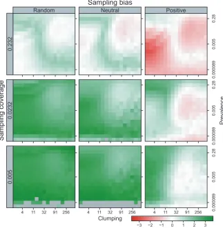
Performance was not consistent across species (Figure 7). Downscaling produced a rather unusual ‘yin‐and‐yang’ pattern of ac‐ curacy where downscaling tended to under‐predict for clumped, me‐ dium‐high prevalence species but over‐predict for dispersed low‐medium prevalence species, when sampling coverage was high (upper row in Figure 7). At lower sampling coverages (lower rows), downscaling tended to under‐predict at all but very low prevalence

F I G U R E 5  The accuracy of predicted occupancy at a grain size of 1 × 1, measured as log(predicted) – log(true) occupancy, from downscaling after subsampling (coverage = 0.0232) using three sampling biases, random, neutral and positive. Downscaling models were fitted to atlas data created at four grain sizes. Each atlas was then aggregated further to larger grain sizes to produce between three to six grain sizes for fitting

–5

05

–5

05

4 8 16 32

–5

05

log(predicted) - log(true) occupanc

y

Atlas scale

3 fitting scales 4 fitting scales 5 fitting scales 6 fitting scales Random sampling

values. We were often unable to provide predictions for extremely low prevalence species under random or regional sampling with low effort due to the scale of endemism preventing model fitting.

Occupancies predicted through downscaling were substantially closer to true occupancy than the raw‐counts method unless sampling coverage was very high, or at lower coverages if there was a positive sampling bias and species were highly clumped (Figure 8).

4 

|

 DISCUSSION

The area occupied by a species is one of the most widely ap‐ plied estimates of a species’ conservation status (Gaston & Fuller, 2009). However, the recommended method of measurement by

summing the area of occupied cells of a 2 × 2 km grid is inaccurate where there are large sampling gaps. A more accurate estimate can be made if occurrences are aggregated across larger spatial (and temporal) scales to create atlas scale data, reducing the num‐ ber of false absences (Figures S2.1–S2.3). We can then fit likely functions to the OAR at large‐grain sizes, where accuracy is high, and downscale them to predict occupancy at the fine grain size required by IUCN.

There are numerous challenges to this approach, listed in the introduction, that have been explored here. These questions have been impossible to address using real species data as so few spe‐ cies have been mapped at sufficiently high resolution and accuracy across large extents, but can be approached using virtual species as demonstrated here.

F I G U R E 6  Accuracy of predicted occupancies at a grain size of 1 × 1, measured as log(predicted) ‐ log(true) occupancy, using ensemble downscaling (red) or raw‐counts (grey), after three subsampling biases (random, neutral and positive) and six sampling coverages (0.005, 0.0107, 0.0232, 0.05, 0.107 and 0.232). The grain size that atlases were aggregated were run‐specific, defined as the largest scale that still allowed for modelling before the scale of saturation or endemism was reached

−4

−2

02

2

−4

−2

0

0.005 0.0107 0.0232 0.05 0.107 0.232

−4

−2

02

log(predicted) - log(true) occupanc

y

Random sampling

Positive sampling bias

Neutral sampling bias

4.1 

|

 Selecting the appropriate atlas scale

Published biodiversity atlases use grain sizes that are understandably standardized across species and highly correlated with atlas extent (Gibbons et al., 2007). In parallel, the open data revolution allows the creation of biodiversity ‘atlases’ for specific objectives directly from distribution data stored in online repositories, allowing greater free‐ dom in the choice of grain and extent. We found that for an atlas to be relatively accurate (i.e. have a limited number of false absences), not only is the sampling coverage and bias critical to selecting grain size, but this scale should be specific to the species’ prevalence and clumping (Figures S2.1–S2.3). For example, accurate atlas data can be generated at fine grains for common, clumped species but if species are rare and dispersed atlas data may be inaccurate even at large‐grain sizes and high sampling coverage.

Issues are further complicated by a species reaching the scale of either saturation or endemism before enough scales are present to fit downscaling models. In this study, we used the largest grain size that still allowed for modelling, but in our example, this led to very small grain sizes for species with very low prevalence. During Red List assessments, if a species reaches the scale of endemism at a fine grain size where sampling coverage is believed to be too low to

generate accurate atlas data, this may be an appropriate reason to assign the species as Data Deficient with regard to AOO.

4.2 

|

 Predicting fine‐scale occupancy

In the majority of cases for our virtual species, the estimates from en‐ semble downscaling were more accurate than were the raw‐counts method but downscaling is still likely to underestimate AOO to some extent (Figures 6 and 8), unless models that systematically over‐predict AOO given perfect data are utilized (Figure S2.16). Prevalence is an im‐ portant indicator of downscaling accuracy (Groom et. al., 2018), but we also found that degree of aggregation will impact the ability to accurately recover the OAR. For example, even given perfect data, downscaling over‐predicts the AOO of scarce, dispersed species but under‐predicts the AOO of abundant, clumped species (Figures S2.9–S2.11).

Underestimation of AOO was greater the lower the sampling coverage (Figure 7) but to a large extent this is due to atlas data at even large‐grain sizes containing a large proportion of false absences (Figures S2.4–S2.6), as underestimation was reduced when a positive sampling bias was ap‐ plied. Every effort should therefore be made to ensure atlas data are ac‐ curate before downscaling is attempted. The increased accuracy through downscaling does come, however, with increased variance (Figure 6).

F I G U R E 7  Accuracy of the downscaled predicted occupancy calculated as log(predicted) – log(true) occupancy for three sampling biases (random, neutral and positive) and three sampling coverages (0.005, 0.0232, 0.232). Blue cells are where downscaling under‐predicted occupancy, orange cells are where downscaling over‐predicted occupancy, and white cells are where occupancy is accurately predicted. Grey cells indicate species where <5 of the replicates could be modelled using downscaling

4 11 32 91 256 4 11 32 91 256 4 11 32 91 256

Random

Sampling bias

0.23

2

0.0232

0.005

50

0.

08

2.

0

98

00

00.

0

Clumping

Prevalence

50

0.

08

2.

0

98

00

00.

0

50

0.

08

2.

0

98

00

00.

0

Sampling coverage

−4 −2 0 2 4

4.3 

|

 Guidelines on downscaling the OAR

The most appropriate approach to estimating AOO should, as far as possible, vary depending upon the characteristics of the species’ dis‐ tribution, the expected sampling coverage and any suspected spatial sampling bias (Table 1). More generally, we propose the following recommendations:

• Where sampling coverage is low, downscaling provides a better estimate of AOO than the raw‐counts method does, but it is still likely to be an underestimate of true AOO (Figures 6 and 8). • Where sampling coverage is very high, and particularly where any

sampling bias is likely to be positive to the species distribution, it may be better to use the raw‐counts method (Figure 8).

• An accurate estimate of AOO is more likely using atlas data at larger grain sizes, but the estimates have greater uncertainty from the downscaling predictions (we must extrapolate further back; Figure 5).

• Where possible downscaling accuracy will be increased by using more scales for fitting, but this should not be done at the expense of using a finer‐grained atlas (Figure 5).

• Where the scale of endemism is reached at fine grain sizes be‐ fore accurate atlas data can be generated, it may be appro‐ priate to assign the species as Data Deficient with regard to Criterion B2.

• Where no other information on the appropriate atlas grain size is available, atlas data should be generated at the largest scale that still allows for modelling before the scale of saturation or ende‐ mism is reached, providing this will not result in very fine grain sizes.

• Care should be taken when using downscaling to assess trends over time, as occupancy changes will be manifested over longer time periods at coarse grains (regional extinctions/colonizations) than at fine grains (local extinctions/colonizations; Hartley & Kunin, 2003).

4.4 

|

 Potential improvements and future directions

Where the downscaling approach could provide additional informa‐ tion over the raw‐counts method is to give an estimate of uncertainty or error around the measurement of AOO, which is not provided by current methods but could be critical when determining if there are trends in changing AOO over time (Akçakaya et al., 2000). There are two errors associated with downscaling.

The first is the error within the downscaling models, which are relatively predictable at least in the direction of error (Figure S2.16; Groom et. al., 2018). Here, we also show that variation between models is dependent upon the species’ prevalence and clumping, as some models appear to struggle to recover the shape of certain

F I G U R E 8  Accuracy of the downscaled predicted occupancy against occupancy calculated using raw‐counts for three sampling biases (random, neutral and positive) and three sampling coverages (0.005, 0.0232 and 0.232). Green cells are species where, on average, using downscaling produced more accurate predictions of occupancy, and red cells are where the raw‐count method produced more accurate predictions. Grey cells for a species are where <5 of the replicates could be modelled using downscaling

Accuracy compared to raw count

4 11 32 91 256 4 11 32 91 256 4 11 32 91 256

Random

Sampling bias

0.23

2

0.0232

0.005

50

0.

08

2.

0

98

00

00.

0

Clumping

Prevalenc

e

50

0.

0

82.

0

98

00

00.

0

50

0.

08

2.

0

98

00

00.

0

Sampling coverage

OARs. Error will also increase with the distance of extrapolation (the larger the atlas scale, Figure 5). To some extent, by exploring a range of possible OARs in simulations such as these, we can therefore pre‐ dict the uncertainty of our estimates given the species’ characteris‐ tics in the atlas data and could weight models during the averaging of the ensemble process accordingly.

The second uncertainty is associated with generating coarse‐ grain atlas data without sampling gaps and is more difficult to es‐ timate as generally we cannot distinguish true absences from areas that have not been sampled. Published atlases ensure accuracy through the accumulation of data over long time periods, but they are generally confined only to well‐known taxa in well‐recorded regions. Unfortunately, for less well‐recorded taxa, particularly in the tropics, the majority of species are represented by fewer than 30 records (Brummitt, Bachman, Aletrari, et al. 2015a; Brummitt, Bachman, Griffiths‐Lee, et al., 2015b).

The issue is exacerbated in that sampling coverage will also be uneven and likely to be spatially biased. It is extremely difficult to estimate sampling coverage or bias from the presence‐only data generally available from biological records, although some models are available that utilize information from the records of similar taxa to ascertain this (Isaac et al., 2014). We urge those that collect bio‐ logical records data to also collect and publish absences where they are certain, as absence data are just as valuable as presence data in nearly all applications for predicting species distributions.

Finally, downscaling methods themselves could also be devel‐ oped further. For example, models could account for potential false absences in the data if we know sampling to be low in particular regions, randomly assigning a presence or absence to uncertain atlas cells. Repeated many times this could produce a distribution of predicted occupancies. Additionally, although most downscaling models account for saturation (occupancy cannot exceed one), none account for the ‘slope of endemism’ where the maximum slope pos‐ sible is when only one of four cells at grain size n is occupied for each cell occupied at grain size n + 1. Therefore, some models pro‐ duce OARs that we know to be impossible. In such cases, the log–log slopes could be set at 0.25.

5 

|

 CONCLUSION

Downscaling occupancy from coarse‐grain atlas data is potentially a valuable method for estimating AOO in IUCN Red List assessments. In previous studies and here we have:

1. Created a new R package which makes ten published down‐ scaling models accessible (Marsh et al., 2018).

2. Shown that an ensemble approach can accurately predict the oc‐ cupancy of a large number of real species (Groom et al., 2018). 3. Shown that for many virtual species, differing in their prevalence

and clumping, ensemble downscaling can fill in information gaps resulting from low sampling coverage and spatial biases better than the currently advocated method of using raw‐counts (Figure 6).

4. Provided information on the limitation of downscaling and guide‐ lines on when it should and should not be used (Table 1).

Given the increased availability of open‐access biodiversity data that allows considerable freedom in creating bespoke atlas data, the potential to automate the fitting of downscaling models, and their ability to provide a more accurate AOO estimate at the rec‐ ommended scale of 2 × 2 km, we hope that downscaling can use‐ fully contribute to the IUCN Red Listing toolbox. We note that downscaling is only one of the tools suggested in the literature to assess AOO (Marsh et. al., in review). Which of these methods is the most appropriate for various species under various sampling scenarios remains under‐explored. Repeating a similar analysis with virtual species for a wide range of AOO methods may re‐ veal further methods that are complimentary to one another, each more suitable for different species and data characteristics, and lead to more holistic guidelines.

ACKNOWLEDGEMENTS

This work was financed by the EU BON project (www.eubon.eu) that is a 7th Framework Programme project funded by the European Union under Contract No. 308454. The authors would like to thank two anonymous referees and to acknowledge the use of the University of Oxford Advanced Research Computing (ARC) facility in carrying out this work. http://dx.doi.org/10.5281/zenodo.22558 .

ORCID

Charles J. Marsh https://orcid.org/0000‐0002‐0281‐3115

Yoni Gavish https://orcid.org/0000‐0002‐6025‐5668

William E. Kunin https://orcid.org/0000‐0002‐9812‐2326

REFERENCES

Akçakaya, H. R., Ferson, S., Burgman, M. A., Keith, D. A., Mace, G. M., & Todd, C. R. (2000). Making consistent IUCN classifications under uncertainty. Conservation Biology, 14(4), 1001–1013. https ://doi. org/10.1046/j.1523‐1739.2000.99125.x

Azaele, S., Cornell, S. J., & Kunin, W. E. (2012). Downscaling species occupancy from coarse spatial scales. Ecological Applications, 22(3), 1004–1014. https ://doi.org/10.1890/11‐0536.1

Barwell, L. J., Azaele, S., Kunin, W. E., & Isaac, N. J. B. (2014). Can coarse‐ grain patterns in insect atlas data predict local occupancy? Diversity

and Distributions, 20(8), 895–907. https ://doi.org/10.1111/ddi.12203

Beck, J., Boller, M., Erhardt, A., & Schwanghart, W. (2014). Spatial bias in the GBIF database and its effect on modeling species’ geo‐ graphic distributions. Ecological Informatics, 19, 10–15. https ://doi. org/10.1016/j.ecoinf.2013.11.002

Brummitt, N. A., Bachman, S. P., Aletrari, E., Chadburn, H., Griffiths‐Lee, J., Lutz, M., … Lughadha, E. M. N. (2015a). The Sampled Red List Index for plants, phase II: Ground‐truthing specimen‐based conser‐ vation assessments. Philosophical Transactions of the Royal Society B: Biological Sciences, 370(1662), 1–11.

global assessment for the IUCN Sampled Red List Index for Plants.

PLoS ONE, 10(8), e0135152.

Freitag, S., Hobson, C., Biggs, H. C., & van Jaarsveld, A. S. (1998). Testing for potential survey bias: The effect of roads, urban areas and nature reserves on a southern African data set. Animal Conservation, 1(2), 119–127. Gaston, K. J. (1991). How large is a species’ geographic range? Oikos,

61(3), 434–438. https ://doi.org/10.2307/3545251

Gaston, K. J. (1994). Measuring geographic range sizes. Ecography, 17(2), 198–205. https ://doi.org/10.1111/j.1600‐0587.1994.tb000 94.x Gaston, K. J. (1996). Species‐range‐size distributions: Patterns, mecha‐

nisms and implications. Trends in Ecology and Evolution, 11(5), 197– 201. https ://doi.org/10.1016/0169‐5347(96)10027‐6

Gaston, K. J., & Fuller, R. A. (2009). The sizes of species’ geo‐ graphic ranges. Journal of Applied Ecology, 46(1), 1–9. https ://doi. org/10.1111/j.1365‐2664.2008.01596.x

Gaston, K. J., & Lawton, J. H. (1990). Effects of scale and habitat on the relationship between regional distribution and local abundance.

Oikos, 58(3), 329–335. https ://doi.org/10.2307/3545224

Gibbons, D. W., Donald, P. F., Bauer, H., Fornasari, L., & Dawson, I. K. (2007). Mapping avian distributions: The evolution of bird atlases. Bird

Study, 54, 324–334. https ://doi.org/10.1080/00063 65070 9461492

Graham, C. H., & Hijmans, R. J. (2006). A comparison of methods for mapping species ranges and species richness. Global Ecology and Biogeography,

15(6), 578–587. https ://doi.org/10.1111/j.1466‐8238.2006.00257.x Groom, Q., Marsh, C. J., Gavish, Y., & Kunin, W. E. (2018). How to predict fine

resolution occupancy from coarse occupancy data. Methods in Ecology and

Evolution, 9, 2273–2284. https ://doi.org/10.1111/2041‐210X.13078

Hartley, S., & Kunin, W. E. (2003). Scale dependence of rarity, extinction risk, and conservation priority. Conservation Biology., 17, 1–12. He, F., & Condit, R. (2007). The distribution of species: Occupancy,

scale, and rarity. In D. Storch, P. Marquet, & J. Brown (Eds). Scaling

Biodiversity, (pp. 32–50). Cambridge, UK: Cambridge University Press.

Hortal, J., Jiménez‐Valverde, A., Gómez, J. F., Lobo, J. M., & Baselga, A. (2008). Historical bias in biodiversity inventories affects the ob‐ served environmental niche of the species. Oikos, 117(6), 847–858. https ://doi.org/10.1111/j.0030‐1299.2008.16434.x

Isaac, N. J. B., & Pocock, M. J. O. (2015). Bias and information in biologi‐ cal records. Biological Journal of the Linnean Society, 115(3), 522–531. https ://doi.org/10.1111/bij.12532

Isaac, N. J. B., van Strien, A. J., August, T. A., de Zeeuw, M. P., & Roy, D. B. (2014). Statistics for citizen science: Extracting signals of change from noisy ecological data. Methods in Ecology and Evolution, 5(10), 1052–1060. https ://doi.org/10.1111/2041‐210X.12254

IUCN (2001). IUCN Red List Categories and Criteria: Version 3.1, 2nd ed. Gland, Switzerland and Cambridge, UK: IUCN.

IUCN (2017). Guidelines for Using the IUCN Red List Categories and Criteria. Version 12. Prepared by the Standards and Petitions Subcommittee. Retrieved from http://www.iucnr edlist.org/docum ents/RedLi stGui delin es.pdf Kéry, M. (2002). Inferring the absence of a species: A case study

of snakes. The Journal of Wildlife Management, 66(2), 330–338. https ://doi.org/10.2307/3803165

Kunin, W. E. (1998). Extrapolating species abundance across spatial scales. Science, 281(5382), 1513–1515.

Kunin, W. E., Hartley, S., & Lennon, J. J. (2000). Scaling down: On the Challenge of estimating abundance from occurrence patterns. The

American Naturalist, 156, 560–566. https ://doi.org/10.1086/303408

Ladle, R. J., & Hortal, J. (2013). Mapping species distributions : Living with uncertainty. Frontiers of Biogeography, 5(1), 8–9.

Marsh, C. J., Barwell, L., Gavish, Y., & Kunin, W. E. (2018). Downscale: An R package for downscaling species occupancy from coarse‐grain data to predict occupancy at fine‐grain sizes. Journal of Statistical Software, 86(3), 1–20.

Mauri, A., Strona, G., & San‐Miguel‐Ayanz, J. (2017). EU‐Forest, a high‐ resolution tree occurrence dataset for Europe. Scientific Data, 4, 160123. https ://doi.org/10.1038/sdata.2016.123

Moerman, D. E., & Estabrook, G. F. (2006). The botanist effect: Counties with maximal species richness tend to be home to universities and botanists. Journal of Biogeography, 33(11), 1969–1974. https ://doi. org/10.1111/j.1365‐2699.2006.01549.x

Powney, G. D., & Isaac, N. J. B. (2015). Beyond maps: A review of the applications of biological records. Biological Journal of the Linnean

Society, 115(April 2015), 532–542. https ://doi.org/10.1111/bij.12517

R Core Team (2017). R: A language and environment for statistical comput-ing. Austria, Vienna:R Core Team.

Reddy, S., & Dávalos, L. M. (2003). Geographical sampling bias and its implications for conservation priorities in Africa. Journal of

Biogeography, 30(11), 1719–1727.

Rivers, M. C., Taylor, L., Brummitt, N. A., Meagher, T. R., Roberts, D. L., & Lughadha, E. N. (2011). How many herbarium specimens are needed to detect threatened species? Biological Conservation, 144, 2541–2547. https ://doi.org/10.1016/j.biocon.2011.07.014

Stropp, J., Ladle, R. J., M. Malhado, A. C., Hortal, J., Gaffuri, J., H. Temperley, W., … Mayaux, P. (2016). Mapping ignorance: 300 years of collecting flowering plants in Africa. Global Ecology

and Biogeography, 25(9), 1085–1096. https ://doi.org/10.1111/

geb.12468

Visconti, P., Di Marco, M., Álvarez‐Romero, J. G., Januchowski‐Hartley, S. R., Pressey, R. L., Weeks, R., & Rondinini, C. (2013). Effects of errors and gaps in spatial data sets on assessment of conservation progress.

Conservation Biology, 27(5), 1000–1010. https ://doi.org/10.1111/

cobi.12095

Willis, F., Moat, J., & Paton, A. (2003). Defining a role for herbarium data in Red List assessments: A case study applying Plectranthus from eastern and southern tropical Africa. Biodiversity and Conservation,

12(7), 1–13.

BIOSKETCH

Charlie Marsh is an ecologist interested in how biodiversity and ecosystem function are affected by anthropogenic disturbance, particularly fragmentation and habitat modification. Recently, the focus has been on the spatial scaling of ecological processes, and decoupling the effects of scales of observation from inter‐ pretations of spatial patterns of diversity. This used to involve lots of exciting running around rain forests, but sadly mainly in‐ volves computer simulations these days.

Author contributions: All authors conceived the idea and de‐ signed the simulations. C.J.M. and Y.G. wrote the scripts and car‐ ried out the analyses. C.J.M. led the writing with input from all authors.

SUPPORTING INFORMATION

Additional supporting information may be found online in the Supporting Information section at the end of the article.