Modelling visual-vestibular integration and behavioural adaptation in the driving simulator

Modelling visual-vestibular integration and behavioural

adaptation in the driving simulator

Gustav Markkula

a,⇑

, Richard Romano

a

, Rachel Waldram

b

, Oscar Giles

a

, Callum Mole

b

,

Richard Wilkie

b

a

Institute for Transport Studies, University of Leeds, LS2 9JT Leeds, United Kingdom b_{School of Psychology, University of Leeds, LS2 9JT Leeds, United Kingdom}

a r t i c l e i n f o

Article history:

Received 7 November 2018

Received in revised form 15 April 2019 Accepted 24 July 2019

Keywords:

Multisensory integration Motion scaling Driver model Steering Slalom

a b s t r a c t

It is well established that not only vision but also other sensory modalities affect drivers’ control of their vehicles, and that drivers adapt over time to persistent changes in sensory cues (for example in driving simulators), but the mechanisms underlying these behavioural phenomena are poorly understood. Here, we consider the existing literature on how driver steering in slalom tasks is affected by down-scaling of vestibular cues, and propose, for the first time, a computational model of driver behaviour that can, based on neurobiologically plausible mechanisms, explain the empirically observed effects, namely: decreased task performance and increased steering effort during initial exposure, followed by a partial reversal of these effects as task exposure is prolonged. Unexpectedly, the model also repro-duced another previously unexplained empirical finding: a local optimum for motion down-scaling, where path-tracking is better than when one-to-one motion cues are avail-able. Overall, our findings suggest that: (1) drivers make direct use of vestibular informa-tion as part of determining appropriate steering acinforma-tions, and (2) moinforma-tion down-scaling causes a yaw rate underestimation phenomenon, where drivers behave as if the simulated vehicle is rotating more slowly than it is. However, (3) in the slalom task, a certain degree of such underestimation brings a path-tracking performance benefit. Furthermore, (4) behavioural adaptation in simulated slalom driving tasks may occur due to (a) down-weighting of vestibular cues, and/or (b) increased sensitivity in timing and magnitude of steering corrections, but (c) seemingly not in the form of a full compensatory rescaling of the received vestibular input. The analyses presented here provide new insights and hypotheses about simulated driving and simulator design, and the developed models can be used to support research on multisensory integration and behavioural adaptation in both driving and other task domains.

Ó2019 The Authors. Published by Elsevier Ltd. This is an open access article under the CC BY license (http://creativecommons.org/licenses/by/4.0/).

1. Introduction

Driving simulators can be valuable tools for research on driver behaviour, industrial prototyping of vehicles, and training of drivers (Fisher, Rizzo, Caird, & Lee, 2011), but only as long as the realism of the simulated driving is satisfactory for the application at hand. For this reason, research into driving simulator realism and validity is an active field of work. This is true

https://doi.org/10.1016/j.trf.2019.07.018

1369-8478/Ó2019 The Authors. Published by Elsevier Ltd.

This is an open access article under the CC BY license (http://creativecommons.org/licenses/by/4.0/).

⇑ Corresponding author.

E-mail address:[email protected](G. Markkula).

Contents lists available atScienceDirect

Transportation Research Part F

not least when it comes to themotion cueingin motion-based simulators; i.e., how to best move the simulator within its limited motion envelope, to create a maximally realistic experience of vehicle movement for the driver, and to elicit objec-tive driver behaviour that is similar to that in a real vehicle (Fischer, Seefried, & Seehof, 2016; Salisbury & Limebeer, 2017; Siegler, Reymond, Kemeny, & Berthoz, 2001).

Typical motion cueing algorithms attempt to leverage the properties and limitations of the vestibular (motion) sensory organs in the inner ear, theotolithsandsemicircular canals, and these systems are relatively well understood and have been modelled in mathematical detail (Hosman, 1996; Nash, Cole, & Bigler, 2016). However, much less is known about (i) how drivers then integrate this vestibular information with information from other sensory modalities (e.g., vision) to support vehicle control, (ii) how these processes are affected by the specific nature of the non-perfect motion cues being provided in a given simulator, and (iii) how drivers adapt over time to such imperfections. A quantitative model of driver behaviour that successfully captured such aspects of multisensory integration and behavioural adaptation would be an eminent tool for improving simulators and motion cueing algorithms. The present paper proposes such a model, and tests it against empirical findings from the literature on driving in slalom tasks. Below, the specific aims and structure of this paper will be described, after first providing brief overviews of existing empirical knowledge about drivers’ response to down-scaled motion (an important special case of motion cueing), and existing models of multisensory integration and driver steering.

1.1. Studies on simulator motion scaling

Most motion cueing algorithms include some element oflinear down-scalingof the actual motion of the vehicle, to stay within the motion envelope of the simulator, even all the way down to zero motion scaling in fixed base simulators. One often observed effect of down-scaled or zero motion is that drivers adopt more aggressive driving strategies (higher speeds and/or tighter curve-taking; Berthoz et al., 2013; Correia Grácio, Wentink, Valente Pais, Van Paassen, & Mulder, 2011; Jamson, 2010; Siegler et al., 2001), and that the control of the vehicle generally becomes less accurate and more effortful (Berthoz et al., 2013; Jamson, 2010; Repa, Leucht, & Wierwille, 1982). This may however be dependent on the specific driving task, sinceWilkie and Wann (2005)found no effect of motion scaling on behaviour in a simple task where participants steered towards a single target.

One type of task where reliable effects have been found, and which is of particular interest in the context of motion scal-ing, isslalomdriving. This task is experimentally useful because, when driven at constant or near-constant speed in a sim-ulator, the motion cueing algorithm can be simplified to direct linear scaling only, isolating the effect of motion scaling on behaviour from other types of motion manipulations that are otherwise often applied (e.g.,tilt coordinationandwashout;

Jamson, 2010). Consequently, many authors have studied how driver behaviour in slalom tasks is affected by variations

in motion scaling, providing converging evidence for a set of behavioural phenomena: Steering effort, for example measured as steering reversal rates or high frequency steering content, generally increases when motion cues are removed (Correia Grácio et al., 2011; Feenstra, van der Horst, Grácio, & Wentink, 2010; Savona et al., 2014), and task performance, objectively measured or subjectively assessed, generally deteriorates (Berthoz et al., 2013; Correia Grácio et al., 2011), although not always (Savona et al., 2014). Taken together, these findings suggest that in normal driving, drivers integrate visual and vestibular cues, and when vestibular cues are removed, task performance becomes more challenging. However, after repeated exposure to the slalom task, control efforts decrease (Feenstra et al., 2010) and task performance improves (Correia Grácio et al., 2011), suggesting some form of behavioural adaptation over time to the lack of vestibular cues. For motion scaling between zero and one, there are reports from several studies of a local optimum, in the 0.4–0.8 range, where task performance and subjective preferences peak (Berthoz et al., 2013; Savona et al., 2014), and in one case this local opti-mum was also observed for steering effort (Savona et al., 2014). Different theories have been proposed for why drivers prefer and perform the slalom best at somewhat down-scaled motion cues; here a novel explanation of this phenomenon will be provided, suggesting that it may be a direct effect of multisensory integration.

1.2. Models of multisensory integration and steering

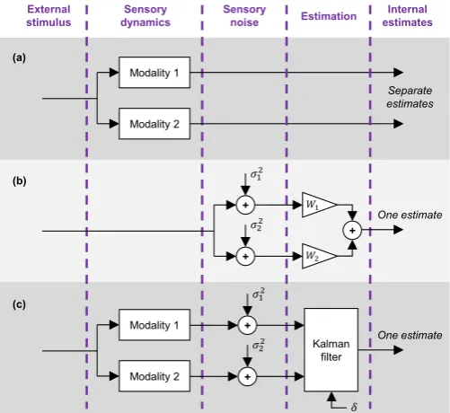
In research focusing on perception and psychophysics, on the other hand, the type of model illustrated inFig. 1(b) has been more common. This model disregards sensory dynamics and instead emphasises thesensory noisepresent in the dif-ferent modalities; it has been repeatedly shown that humans and other animals often behave as (near-) ideal Bayesian obser-vers, by engaging in (near-)optimal cue integration, where the sensory cues are weighted by their reliabilities, i.e., the inverse of their respective noise variances (Wi/1=

r

2i inFig. 1).Fetsch, DeAngelis, and Angelaki (2013)andNash et al. (2016) pro-vide reviews of this literature from neurobiological and vehicle control perspectives, respectively.

The model illustrated inFig. 1(c) is a combination of the models in (a) and (b), with the optimal cue integration being carried out as part of a Kalman filter. This type of scheme has been common in optimal control theoretic models of various sensorimotor control tasks (Franklin & Wolpert, 2011; van Beers, Baraduc, & Wolpert, 2002; van der Kooij, Jacobs, Koopman, & Grootenboer, 1999), and was recently applied byNash and Cole (2017)in their multisensory optimal control model of dri-ver steering. In these models, the Kalman filter makes use of knowledge of the own past control actions as well as internal forward models of the system being controlled, including the own sensory dynamics. Therefore, as long as any changes in a vehicle’s state are mainly caused by the driver’s own control, and not by external perturbations such as potholes or wind gusts, the Kalman filter inFig. 1(c) can compensate for the sensory dynamics, essentially reducing the model to the situation inFig. 1(b). Since the empirical literature on slalom driving does not emphasise external perturbations, the scheme inFig. 1

(b) will be adopted here.

Predictive forward models, orgenerativemodels, are also emphasised in so-calledpredictive processingaccounts of brain function (e.g.,Bogacz, 2017; Friston, 2005). These accounts suggest neurobiologically plausible mechanisms for how the brain can learn its own sensory reliabilities, by first learning a generative model, and then observing deviations between received and predicted sensory data. This type of mechanism will also be leveraged here.

1.3. Aims of this paper

[image:3.544.149.400.58.288.2]

This paper proposes, for the first time, a driver steering model that reproduces, and therefore provides stringent and con-crete explanations for, the observed empirical effects of motion down-scaling in simulators, specifically (i) how humans first react to down-scaled motion cues, and (ii) how this behaviour changes with repeated task exposure. To address this aim, the model needs to account both for multisensory integration and some form of behavioural adaptation. Here, the neurobiolog-ically plausible framework for intermittent control proposed byMarkkula et al. (2018a)was used as a starting point, since it lends itself naturally to a range of plausible potential mechanisms for behavioural adaptation. From a modelling perspective, the novelty lies in the extension of the existing framework with these adaptation mechanisms (as far as we are aware this is the first ever model of behavioural adaptation in steering), as well as with the optimal cue integration mechanisms reviewed Fig. 1.Three different types of modelling schemes for multisensory integration. (a) Sensory dynamics models only; common in aircraft pilot models in research on flight simulators. (b) Modality-dependent sensory noise (variancesr2

1andr22) and optimal cue integration; common in psychophysical studies

above. It was not an original aim of this work to study the phenomenon of a local optimum in slalom motion down-scaling, but as will become clear below, the model turns out to be applicable also to this phenomenon.

Below, the steering model is first introduced. Then, results from model simulations are presented, before a discussion and conclusions are provided.

2. Theory and methods

This section describes the proposed driver steering model, illustrated inFig. 2, as well as the model simulations carried out to study the model’s behaviour.

2.1. Driver steering model

2.1.1. Slalom desired path

The model adopts the commonly used concept of adesired path(Plochl & Edelmann, 2007) to define the sinusoidal slalom task. The exact setup of this task was here based on (Feenstra et al., 2010): 62.5 m spacing between cones, 3 m lateral ampli-tude, and the task was carried out at a constant longitudinal speed of 70 km/h.

2.1.2. Intermittent control framework

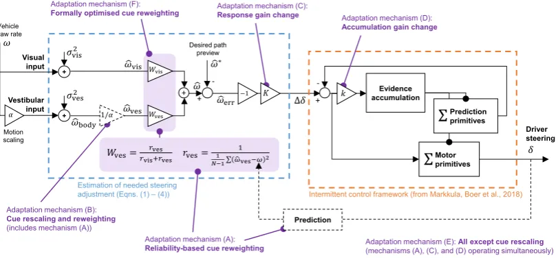
As mentioned, the model builds on a framework for intermittent sensorimotor control, introduced and described in detail byMarkkula, Boer et al., (2018), and schematically illustrated here in the rightmost part ofFig. 2. In brief, this framework assumes that a continuously calculated estimate of currently needed control adjustmentDdis compared to a prediction ofDd, to yield a prediction error. This prediction error is then fed, with a gaink, into anevidence accumulation(also known asdrift diffusion) step where it is integrated over time to a threshold of1, to decide on when a control adjustment is needed. This is in line with neurobiologically proven mechanisms for how the brain makes decisions based on noisy sensory data (Gold & Shadlen, 2007; Purcell et al., 2010; Ratcliff, Smith, Brown, & McKoon, 2016). In theMarkkula, Boer et al., (2018)

[image:4.544.69.475.419.607.2]

framework, when the evidence accumulation has integrated to threshold, the integrator is reset to zero, a control adjustment is initiated, and a prediction is made of howDdwill be affected over time by the new control adjustment. The adjustment as such is applied in the form of a kinematicmotor primitive(Giszter, 2015), here a fixed-duration (DT= 0.4 s, based on the find-ings byBenderius & Markkula, 2014) stepwise change of the steering wheel angle, with a bell-shaped rate profile and with amplitude obtained directly from the currentDdprediction error, plus signal-dependent motor noise (Franklin & Wolpert, 2011). Also theDdprediction is obtained as a superposition of stereotyped ‘‘prediction primitives”, mimicking neurobiolog-ically observedcorollary discharge(Crapse & Sommer, 2008; Requarth & Sawtell, 2014).

Fig. 2.Schematic illustration of the driver steering model tested in this paper. The leftmost part of the figure shows how the model responds to noisy visual and (possibly down-scaled) vestibular cues, creating an estimate of needed steering adjustmentDdby weighting the modality-specific estimates of the true vehicle yaw ratexaccording to an optimal cue integration scheme (reweighting equations shown only for vestibular weights and reliabilitiesWvesandrves),

and then comparing the integrated estimatex^to a desired yaw ratex^_{. The rightmost part of the figure is a simplified illustration of how the intermittent} control framework (described in full detail byMarkkula, Boer et al., 2018) transformsDdinto the steering wheel angled. The various tested behavioural adaptation mechanisms are also indicated in the figure. The 1=acue rescaling gain is shown in dashed line because it is only present in the model when that adaptation mechanism is enabled; when it is not,xves¼xbody. The prediction fromdtoxis shown in dashed line because this prediction is assumed in the

2.1.3. Needed steering adjustment

In the engineering literature, there are several driver steering models (Gordon & Magnuski, 2006; Markkula, Benderius, & Wahde, 2014; Tan & Huang, 2012) on the general form:

D

d¼ K

x

^err¼ Kð

x

^

x

^Þ; ð1Þ

where

_x

^_and

_x

_{^ are desired and actual vehicle yaw rate, as perceived by the driver, andKis a steering response gain. As}

mentioned in the Introduction, there is a considerable literature in the ecological psychology tradition, arguing for the importance of considering what types of information is actually perceptually available to the driver, rather than assuming access to ‘‘engineering quantities” like yaw rate. Interestingly however, it can be shown that models in the ecological psy-chological literature, emphasising more plausible visual inputs such as sight point rotations, can be rewritten on the form of Eq.(1)(Markkula, 2013), so it can be argued that this type of control law is perceptually plausible.

Here, the desired yaw rate

x

^_{is defined as the yaw rate that would take the vehicle back to the desired path in a preview}

timeTP. This formulation has been shown to successfully replicate human slalom steering, withTP2 ½1:4;2:2s (Markkula, Romano, et al., 2018); hereTP= 1.8 s was used.

2.1.4. Visual-vestibular integration

As mentioned above, in this paper we follow the psychophysical literature on optimal cue integration, modelling multi-sensory integration as operating directly on estimates of the external stimulus, in this case vehicle yaw rate:

^

x

¼ Wvis

x

^visþWves

x

^ves

Wvisð

x

visþ

m

visÞ þWvesð

x

vesþ

m

vesÞ;

ð2Þ

where

x

vis¼

x

and

x

ves¼

x

body¼

ax

, with

x

body the actual rotation of the driver’s body,

a

the motion scaling being applied,

x

the yaw rate of the simulated vehicle, and

_m

visand

m

ves being Gaussian white noise with standard deviations

r

visand

r

ves. Optimal cue integration theory prescribes:

Wvis¼ rvis

rvisþrves; Wves¼

rves

rvisþrves; ð3Þ

withrvisandrvesbeing the respective sensory reliabilities (rvis¼

r

2

vis;rves¼

r

ves2). Note that here, the otoliths and semicircular canals are in effect subsumed into a single estimate of yaw rate, since this is all the control law in Eq.(1)needs (but it may also be noted that in a vehicle, lateral acceleration, as sensed by the otoliths, typically provides good information on yaw rate also).

Thus, overall, what is suggested here (in the leftmost dashed box inFig. 2) is that drivers might behave as if (i) they trans-form the neural output from their sensory organs into estimates of yaw rates, presumably considering also predictions based on knowledge of past steering input, (ii) integrate these yaw rate estimates as per Eqs.(2) and (3), and then (iii) compare the result to a visually estimated desired yaw rate, to calculate the needed steering adjustment as per Eq.(1). Note the, ‘‘as if” above; it is not assumed that drivers’ brains necessarily directly perceive and encode things like desired paths or desired or actual yaw rates, only that they behave as if they do.

Here,

_r

vis¼0:5°/s was used, loosely based onNesti, Beykirch, Pretto, and Bülthoff (2015), who found that humans could discriminate between visual rotation stimuli of about 5°/s (at which yaw rates typically peak in the present slalom task) if they were different by 1°/s. The 0.5°/s noise level gives 75 % correct direction classification, by a drift diffusion model such as in the intermittent control framework used here, of a 1°/s stimuli if presented during 10 s, a similar duration of presentation as inNesti et al. (2015).

As for the vestibular noise, the literature on how visual and vestibular sensory systems compare in terms of delays or noise levels provide conflicting information for different types of experimental conditions (Nash et al., 2016), so for simplic-ity we here assume

_r

vis¼

r

ves, to begin with. However, later in this paper we also examine the model’s sensitivity to vari-ations in these noise levels.

It is assumed that when first entering the simulator, the driver’s sensory weightings are preset, based on prior driving experience, in line with the true sensory reliabilities (rvis¼

_r

2

vis;rves¼

r

ves2), which with

r

vis¼

r

vesgivesWvis¼Wves¼0:5.

2.1.5. Behavioural adaptation

As also illustrated inFig. 2, a number of mechanisms for behavioural adaptation are assumed to be operating, alone or in combination:

rvis¼ 1 1

N1 PN

i¼1ðx^vis;ixiÞ

2

rves¼ 1

1

N1 PN

i¼1ðx^ves;ixiÞ 2;

ð4Þ

and the weightsWvisandWvesare then updated in accordance with Eq.(3)before the next simulation run. As long as there is no motion down-scaling (i.e.,

a

¼1), this will just result in the model retrieving approximate estimates of the true inverse noise variances (rvis

_r

2

vis;rves

r

ves2). However, when

a

–1 and

x

ves¼

ax

, the estimation ofrvesis affected by the resulting persistent bias of

x

vesaway from

x

, causing lower vestibular reliabilitiesrvesthe further

a

diverges from unity, i.e., the fur-ther the perceived vestibular cues are from what the driver’s brain would expect based on its past experiences from real driving.

(B) Reinterpreting the down-scaled vestibular cues, byrescalingthe mapping from vestibular organ output to

_x

ves, i.e.,

x

ves¼

x

body=

a

. Since this type of sensory relearning simultaneously scales up the vestibular noise by 1=

a

, it is assumed that it would include appropriate reweighting of cues, i.e., mechanism (A) was also included here.

(C) Adapting the steering response gainK, i.e., increasing or decreasing how much one changes the steering angle for a given perceived yaw rate error

_x

^err.

(D) Adapting the gainkin the evidence accumulation. This can be thought of as adaptingeffortorarousal; increases ink cause the model to apply more frequent (and hence typically smaller) steering adjustments, and vice versa.

The mechanisms (C) and (D) are assumed to operate so as to optimise behaviour towards some goal, here implemented in practice as an exhaustive search over a grid of the optimised parameters, minimising the cost function:

Jtot¼ kpathJpathþksteerJsteer

kpath1

N XN

i¼1 ðyiyiÞ

2_þ ksteer1

T Xn

j¼1 g2

j

ð5Þ

for a simulation of durationT, withNdiscrete simulation time steps, in whichndiscrete steering adjustments with ampli-tudesgjare applied, and with lateral positions of vehicle and desired pathyiandyi, respectively. This is a common form of cost function for optimal control theory models of steering (Nash & Cole, 2017; Plochl & Edelmann, 2007). Note that it is not implied here that the brain performs grid search to change its behaviour; only that it implements some optimisation mech-anism (unspecified here, but see the Discussion) of which the effect is gradual reduction of something likeJtot. The weighting parameters were set tokpath¼1 andksteer¼10 to get similar magnitudes across both cost function terms in typical simula-tions with the model. Later in this paper we also examine the model’s sensitivity to variasimula-tions in these weights.

As will be described under Results below, all of the mechanisms (A), (C), and (D) were found promising individually, but not (B). Therefore, also the following was tested:

(E) All three adaptations (A), (C), and (D) operating simultaneously. Finally, also this mechanism was tested:

(F) Adapting sensory weights not based on estimated reliability as in mechanism (A), but instead to minimiseJtotusing the grid search optimisation described above. The purpose of this test was to investigate whether or not the reliability-based cue reweighting (A) yielded similar results as a formal optimisation of the cue weights.

2.2. Driver-vehicle model simulations

Simulations were run with a linear vehicle model, fitted to multibody simulations of a Jaguar XF driving slaloms, mostly in the linear tyre regime.

For the gainskandK, initial, before-adaptation values for the model were selected as those gains that minimisedJtotfor driving with full motion (

a

¼1); i.e., it was assumed that the driver comes to the simulator with these gains preset based on prior driving experience (and can rapidly adapt to the steering gain of the specific simulated vehicle). In practice, an exhaus-tive grid of values for both gains was searched, with twenty repetitions per gain combination (since the driver model is stochastic) of the

a

¼1 slalom. Optimal model performance was obtained fork¼450 (arbitrary units) andK¼2:04 s. It may be noted that this latter figure is close to the theoretically optimal steering response gain 1/0.510 s = 1.96 s, with 0.510 s1_{being the steady state yaw rate response gain of the vehicle model used in the simulations.}

A number of additional simulated tests were also run, to investigate the model’s sensitivity to the difficulty of the slalom in terms of the distance between cones, the assumed sensory noise levels and cost function weights, and the assumption of intermittent rather than continuous steering control. For this latter test, we replaced the intermittent control part of the model (the right half ofFig. 2) with just a fixed time delay ofDT=2¼0:2 s and a gain 1/DT¼2:5 s1, to obtain a continuous rate of steering wheel changed_; as explained in (Markkula, Boer et al., 2018) this continuous model behaves roughly as an average-filtered version of the intermittent control model. The steering cost for this model was changed, to consider contin-uous steering wheel rates instead of discrete steering wheel adjustments as in Eq.(5):

Jsteer¼1 T

XN

i¼1 _ d2i;

andksteerwas set to 0.1, with the same type of motivation as provided above for the intermittent model.

3. Results

3.1. Impact of motion scaling and behavioural adaptation mechanisms

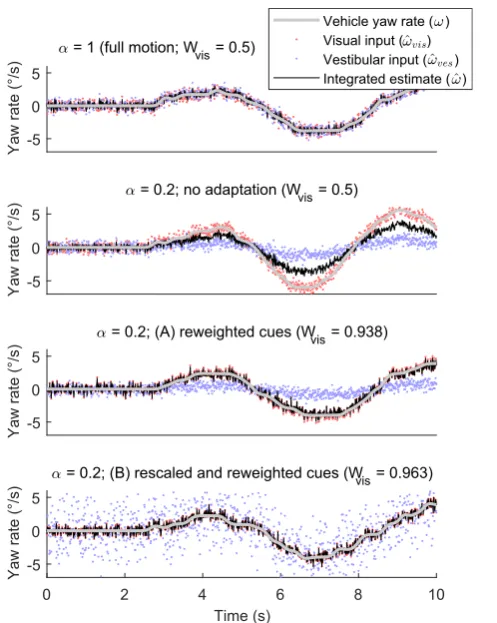
3.1.1. Yaw rate estimation

[image:7.544.154.403.352.664.2]

Fig. 3provides an illustration of the visual-vestibular estimation of yaw rate, from simulations with the model under dif-ferent conditions. The top panel shows a simulation with full motion cues (

a

¼1), the other three are all simulations with down-scaled motion cues (

a

¼0:2). Note that without any adaptation whatsoever (second panel from top), the combined estimate of yaw rate (black line) becomes strongly biased towards zero, away from the true yaw rate (light gray line). This bias all but disappears when reweighting the cues based on prediction-estimated reliabilities (third panel). If rescaling the vestibular cues (bottom panel), a completely non-biased estimate can again be obtained, making what would seem like a theoretically optimal use of the vestibular cue, despite the vestibular noise also becoming visibly inflated by the rescaling.

3.1.2. Model time series behaviour

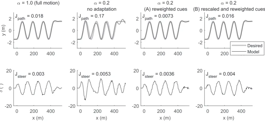
Fig. 4shows example time series behaviour of the model in the same four conditions as inFig. 3. Without any adaptation, the model’s steering becomes unstable when motion is scaled down, resulting in increasing path and steering costs. This instability is counteracted when downweighting vestibular cues, both with or without prior rescaling of the vestibular input, but steering efforts still remain higher than in the full motion case. Note, however, that the lowest path cost is obtained for the simulation with reweighted but not rescaled cues.

3.1.3. Task performance and steering effort

A more complete overview of path-tracking and steering costs, as a function of motion scaling and adaptation mecha-nisms, is provided inFig. 5. It can be noted that, in line with the empirical reports, steering efforts (Jsteer) increase with decreasing

a

, especially for the non-adapted model at low

a

. However, all of the behavioural adaptation mechanisms succeed at improving this situation, which in turn aligns with the empirical reports of decreasing steering efforts after prolonged exposure to the slalom task.

Related patterns can be observed for the path tracking costs (J_path), but with the important difference that for all simula-tions except the cue rescaling adaptation (B), there is a local minimum at

a

2 ½0:6;0:8, i.e., the model reproduces not only the general tendency of worse performance for down-scaled motion, and improvement with adaptation, but also the sub-unity local optimum for motion scaling that has been reported in the empirical literature. After applying the rescaling adaptation (B), however, there is close to zero effect of motion scaling on the model’s path-tracking performance.

Analysing the values of adapted parameters provides further insight into how the adaptation mechanisms operate.Fig. 6

shows that the performance improvements from adapting evidence accumulation and steering response gains are both had by increasing these gains, resulting in more frequent adjustments and higher-amplitude steering adjustments, respectively.

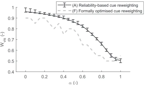
Fig. 7shows that the cue weighting obtained by measuring reliability as deviations from expected sensory input, a type of reliability estimate that should be readily available to the brain, was relatively close to the optimal weighting obtained when formally optimising for minimal costJtot.

3.2. Sensitivity to task and model variations

Fig. 8illustrates the model’s sensitivity to various modifications to the task and the model itself.

3.2.1. Slalom difficulty

Fig. 8a shows that the qualitative behaviour of the model is insensitive to the spacing of the cones in the slalom task. However, the model can be seen to reproduce another empirical observation made bySavona et al. (2014); the motion scal-ing optimum occurs at lower

a

for more difficult slaloms (with shorter cone spacing, requiring higher lateral accelerations).

3.2.2. Sensory noise

[image:8.544.53.490.466.667.2]

As mentioned earlier, it is difficult to know what magnitudes to choose for the sensory noises. However, as long as

r

vis¼

r

ves, changing these up or down does not change the shape of the path-tracking and steering cost curves; these simply go up and down with the noise levels.

[image:9.544.53.493.54.171.2]

However, it could be argued, based on perceptual threshold experiments, that the visual system is more sensitive than the semicircular canals in discrimination of pure yaw motion (Riemersma, 1981; Soyka, Giordano, Barnett-Cowan, & Bülthoff, 2012). Therefore, as shown inFig. 8b, simulations were run where the vestibular noise was increased, while maintaining

r

vis¼0:5=s. The figure shows that doing so maintains the high-level qualitative effects of motion scaling, but the impact of motion scaling is reduced, in the sense that larger reductions in

a

are needed to see an impact. The reason the model responds in this way is that with higher vestibular noise levels, Eq.(3)prescribes lower vestibular sensory weights to begin with, making the model less sensitive to variations in

_a

. One consequence of this phenomenon is that the local optimum for path-tracking cost shifts to lower

a

with increased vestibular noise. As mentioned previously, the empirically observed local path-tracking optimum for

a

is in the 0.4–0.8 range, and the model aligns best with these findings when vestibular noise levels are similar to the visual noise levels (here,

_r

ves¼0:5=s) or up to double the visual noise levels (here,

r

ves¼1=s).

[image:9.544.149.402.208.341.2]

Fig. 5.Costs as a function of motion scaling, for the non-adapted model and for the hypothesised adaptation mechanisms (A)–(E).

Fig. 6.Adapted optimal evidence accumulation gain (k) and steering response amplitude gain (K), as a function of motion scaling. The dotted horizontal line indicates the optimal gains for full motion (a¼1).

[image:9.544.151.401.386.532.2]

3.2.3. Cost function weights

The costJ_totis only used to identify optimal model parameterisations, disregarding the actual value ofJ_tot. Therefore, mod-ifying both cost functions weightskpathandksteerup or down by the same factor does not affect the obtained results, but vary-ing them relative to each other does. However,Fig. 8c shows that this impact is small, even when modifying the ratio ksteer=kpathby as much as a factor ten up or down (from the originalksteer=kpath¼10). With largerksteer, the initial model opti-misation (for

a

¼1) yields a parameterisation with higher accumulator gaink and lower response gainK, thus applying smaller steering corrections more often, which brings downJsteerslightly, at the cost of a small increase inJpath. As can be seen inFig. 8c, the qualitative effects of then reducing

a

and applying adaptation mechanisms remain largely unaffected by theksteer=kpathratio.

3.2.4. Continuous model

Comparing the results for the continuous model inFig. 8d to those for the intermittent model inFig. 5, it can be seen that many but not all of the qualitative phenomena are retained in the continuous model: Steering costs still go up for the non-adapted model with

a

<1, and the sub-unity motion scaling optimum for path-tracking persists, but for the continuous model there is close to zero effect of

a

on steering costs after all of the adaptations.

4. Discussion

4.1. Sensory integration and behavioural adaptation

[image:10.544.47.490.48.335.2]

The model of multisensory integration used here was relatively simple. Nevertheless, the main targeted empirical phe-nomena, in terms of task performance and steering efforts, were all qualitatively captured by the model. Thus, the model analyses provided here suggest that low task performance and high steering efforts upon first exposure to down-scaled motion cues can be understood as drivers responding to these down-scaled cues as if they aredirectly underestimating vehicle yaw rate, and use this underestimation when shaping their steering. As a result, this steering becomes more effortful, and in many cases also more unstable.

Fig. 8.Effects of task and model variations on path-tracking costsJpathand steering costsJsteer, as functions of motion scalinga. Note that for readability,

panels (a)–(c) show results only for the ‘‘no adaptation” and ‘‘cue reweighting” conditions. (a) Impact of slalom cone spacing (42.5 m, 52.5 m, or 62.5 m, as indicated in theJpath panel). (b) Impact of vestibular sensory noise levels (rvesat 0.5°/s, 1°/s, or 1.5°/s, as indicated in theJpath panel;rvis¼0:5=s

throughout). (c) Impact of steering cost weight relative to the path-tracking cost weight (ksteer=kpathat 1, 10, or 100, as indicated in theJsteerpanel). (d)

Results for a simplified, continuous version of the model. TheJpathpanel retains the scale of the corresponding panel inFig. 5, but theJsteerpanel has a

The fact that the analyses support the idea of drivers using the underestimated yaw rates as part of their control is inter-esting in its own right. Much of the existing empirical literature on driving simulator motion can be interpreted conserva-tively in this sense, to say that motion cues mainly cause drivers to change their higher-level strategy in terms of adopted speeds or trajectories, to avoid experiencing large accelerations (Berthoz et al., 2013; Correia Grácio et al., 2011; Jamson, 2010; Siegler et al., 2001), or that motion cues mainly support rejection of unexpected external perturbances like wind gusts (Greenberg, Artz, & Cathey, 2003; Repa et al., 1982). The present model and simulation analyses, together with the existing empirical findings from slalom experiments, instead suggest a stronger account, whereby drivers make direct use of vestibu-lar information as part of shaping their steering to reach their intended targets, also in the absence of any external pertur-bances or high-level adaptations of trajectory or speed. It is clear that existing multisensory models of drivers (Nash & Cole, 2017) and pilots (e.g.,Mulder et al., 2013) also suggest this deep form of involvement of vestibular cues in control, but we are not aware of any prior analysis of empirical data providing support for it in driving.

With respect to behavioural adaptation, the results presented here indicate that especially three mechanisms, or several of them in combination, are candidates for causing the empirically observed effects of repeated task exposure: increased gains in evidence accumulation (mechanism D) or steering response (mechanism C), or sensory cue reweighting based on reliabilities inferred from deviations between received and predicted sensory input (mechanism A). Especially this latter mechanism seems readily implementable in neural systems, and it also provided the most dramatic performance improvements. Interestingly, the cue weights obtained in this way came close to the formally optimal values (mechanism F;Fig. 7); that this would be the case was not clear a priori, since the formally optimal values depend on the specific task and chosen cost function.

Also the increases in accumulator and steering gains can actually be interpreted in neurobiological terms; increases in global cortical arousal by means of broad diffusion of noradrenaline (also known as norepinephrine) has been found to have the specific effect of increasing gains in neuronal response to inputs (Aston-Jones & Cohen, 2005). Thus, it could be hypoth-esised that the driver’s brain may respond to unsatisfactory task performance with release of noradrenaline, increasing the evidence accumulation and response gains.

The present analyses do not provide any conclusive insight into which of the three adaptation mechanisms mentioned above may have been more important in the empirical studies, or whether they were maybe all present simultaneously (mechanism E). However, the results can be taken to suggest that complete rescaling of the vestibular input (mechanism B) may not have occurred in the human drivers in these studies, since if so there would not, according to the model simu-lations, have remained any local optimum in task performance for

a

<1. This leads on to the next section.

4.2. Sub-unity optimum in motion scaling

It was not expected beforehand that the model would exhibit the local performance optimum for sub-unity motion scal-ing. Previously, it has been proposed that this phenomenon might be due to imperfections and false cues in motion systems becoming more prominent at

a

too close to 1, or to motion down-scaling being needed to ensure coherence with underes-timated visual speeds (Berthoz et al., 2013), or to successful control of arms and steering wheel becoming more difficult when the body is subjected to higher and more uncomfortable accelerations (Savona et al., 2014). However, none of these mechanisms were included in the model, yet it still reproduced the phenomenon.

Here, what is happening instead is that the model gets a path-tracking benefit from slightly underestimating the yaw rate in this task. Looking closely at the different vehicle trajectories inFig. 4, or the magnified view inFig. 9, it can be seen that (i) the path tracking cost is to a large extent determined by how well the vehicle’s path is phase-aligned with the desired path, (ii) for

a

¼1, the vehicle trajectory phase is slightly late (reaching apex after the desired path does), and (iii) motion down-scaling shifts the vehicle trajectory to progressively earlier phase, giving rise to the local path tracking optimum. Interest-ingly, whenBerthoz et al. (2013)analysed what caused the path tracking optimum for human drivers in their study, this type of trajectory phase alignment is exactly what they found (see their Fig. 10). In our model, the reason this is happening is that the more the model underestimates its own yaw rate, the earlier and the more vigorously it will respond to the next turn in the slalom, causing the trajectory to reach apex earlier. This explanation also aligns with the analysis of steering angles by

Feenstra et al. (2010, Fig. 4b; also reproduced as Fig. 6 inBerthoz et al., 2013), who found that when motion cues were absent, drivers adjusted their steering more quickly after passing a cone gate. This empirical finding matches what is seen inFig. 9here, and is indeed what one would expect from a driver who perceives that s/he isn’t rotating quickly enough in preparation for the next cone gate.

In sum, from a path-tracking perspective the model captures essentially all aspects of what has been empirically estab-lished with respect to the sub-unity optimum phenomenon: Not only the existence of an optimum, but also its cause being trajectory phase alignment, as well as how the optimum is affected by slalom difficulty (Fig. 8a). Overall, this can be taken to suggest that underestimation of yaw rate (or, as said before, behavingas ifone underestimates yaw rate) may indeed be the mechanism behind this phenomenon also in humans.

Another question raised by the present analyses is to what extent the sub-unity motion scaling optimum phenomenon is particular to slalom tasks. The phase-alignment path-tracking benefit from yaw rate underestimation observed here seems to be rather closely related to the specific nature of this task, such that it might not necessarily generalise.

4.3. Driver steering modelling

We have shown in this paper how the intermittent control framework of Markkula et al. (2018a)can be naturally extended to account for multisensory integration and a number of behavioural adaptation mechanisms; these extensions should be of value in a range of contexts relating to driving simulators and in other application domains.

It is notable, however, that much of the results of the intermittent control model were reproduced also by the continuous model. The main differences, quite expectedly, related to steering effort: In addition to the lack of the putatively effort-related evidence accumulation gain adaptation, which cannot be included in the continuous model, the effect of motion scal-ing on steerscal-ing costs all but disappeared with all behavioural adaptations in the continuous model. Nevertheless, since the continuous model is so simple and easy to implement (just the few operations in the left part ofFig. 2plus a delay and a gain), it seems particularly well suited for use in future studies of multisensory integration in driving simulators.

One limitation of all of the models tested here is that they rely on single point preview. While, as mentioned above, this type of model has been shown to capture many aspects of human steering,Boer (2016)has shown that it cannot replicate certain more advanced, anticipatory human behaviours, such as a ‘‘swing wide” before the first cone gate in a slalom, as an early preparation for thesecondcone gate. However, this type of behaviour does not seem central to our main findings here (regarding effects of motion down-scaling, the sub-unity tracking optimum, and behavioural adaptation mechanisms), since our findings arguably primarily concern the later, ‘‘steady state” oscillatory stage of the slalom.

The main alternative to the models tested here is the one proposed byNash and Cole (2017). This model assumes optimal control in a more complete sense, with access to explicit internal models of the vehicle as well as of the sensory and neuromus-cular dynamics. On a cursory analysis, it seems likely that also this model would exhibit lower performance and higher steering effort when motion is scaled down or turned off. Among the adaptation mechanisms studied here, the combined rescaling and reweighting mechanism (B) would seem to fit especially naturally within the framework. Here, the model behaviour with this mechanism did not align well with the existing empirical findings, but direct testing in model simulation would be needed to see whether it fares better in theNash and Cole (2017)framework. Also the pure cue reweighting adaptation (A) could be used, if the optimal control framework is extended with a similar prediction-based estimation of reliabilities as proposed here. How-ever, the gain adaptations (C) and (D) do not seem readily compatible with theNash and Cole (2017)model.

[image:12.544.159.384.53.268.2]

It would also be interesting to test whether theNash and Cole (2017)model reproduces the sub-unity motion scaling optimum phenomenon. At least in its non-adapted form, this model should also underestimate yaw rate. However, as dis-cussed above, an important part of the reason why our model tracks the desired path better when underestimating yaw rate Fig. 9.The effect of motion scale factoraon the phase of model steeringdand resulting vehicle lateral positiony, across a longitudinal subset of the simulated slalom track. The plotted traces are averages across twenty model simulations for each motion scale factor. The top and bottom panels can be compared to Figs. 10 and 6, respectively, in (Berthoz et al., 2013). The model used here is the intermittent control model, without any behavioural adaptation to the motion down-scaling. The vestibular noise was set torves¼1=s¼2 rvis, resulting in the path-tracking optimum occurring ata¼0:5, as

is because with full motion cues its control is to a certain degree inherently suboptimal (the trajectory phase misalignment), something which,a priori, would not seem to be the case for theNash and Cole (2017)model.

4.4. Future work

As has already been hinted at above, one obvious future direction would be to apply the models proposed here to other tasks besides the slalom. Ideally, one would first generate predictions for these other tasks using the model (perhaps just the continuous version of it, for simplicity), and then investigate whether these predictions are borne out in tests with human drivers. In such empirical work, one could also study the adaptation process itself in more detail, for example to try to dis-tinguish better between the various hypothesised mechanisms for adaptation. Additional adaptation mechanisms are also imaginable. For example, it is possible that drivers respond to down-scaled or otherwise imperfect motion cues by adjusting the overall goals of their driving, something which could be operationalised in the present model as modifications to the cost function weights (kpathandksteer), or even Eq.(5)itself.

The model proposed here could also be applied in development and tuning of motion cueing algorithms, in its present form especially for direct scaling cueing. For example, one could use the model to predict what motion scaling might yield behaviour that is as similar as possible to that in a real vehicle, or to predict how large the differences might be between behaviour before and after adaptation to a certain motion scaling, to get an idea of what motion cueing settings might take longer time to get used to.

If the model is to be used with more complex, arbitrary motion cueing algorithms, for example affecting rotations and translations in different ways, the current simplified approach of capturing all vestibular sensing in just a yaw rate estimate will not be enough, and it needs to be better considered how different types of motion cues are used by drivers when deter-mining the needed steering control. One possibility is theNash and Cole (2017)approach, with sensory dynamics models and inverse model state estimators (modelling scheme (c) inFig. 1). A possible complication here is that empirical observa-tions suggest that rotation and translation cues may not be used by human drivers in precisely the ways suggested by this type of engineering analysis (Lakerveld et al., 2016).

5. Conclusion

We aimed to study visual-vestibular integration and behavioural adaptation in the driving simulator, by modelling human steering behaviour in slalom driving, a type of task that has been much studied in simulators with linearly down-scaled motion cues. To this end, we started from an existing modelling framework for intermittent sensorimotor control, building on concepts such as sensory evidence accumulation, motor primitives, and sensory predictions (corollary dis-charge), and extended it with mechanisms for optimal sensory cue integration and behavioural adaptation. The resulting extended framework, as well as a simplified continuous version of it, seem well suited for future work on multisensory inte-gration and behavioural adaptation in driving simulators and elsewhere.

A key insight from the present work is that much of the empirically observed phenomena in motion down-scaling of sla-lom driving tasks can be explained by ayaw rate underestimationmechanism, whereby drivers respond to down-scaled sim-ulator motion as if they perceived themselves and the simulated vehicle to be rotating more slowly than is the case in the simulated situation. This mechanism explains not only why removing motion cues leads to increased steering efforts and worse path tracking, but also captures a phenomenon for which there has previously been no good explanation: In an inter-mediate range of mild down-scaling, the yaw rate underestimation phenomenon counteracts an inherent suboptimality in the model’s steering behaviour, resulting in improved path tracking.

A range of neurobiologically plausible mechanisms for behavioural adaptation were hypothesised and tested. Out of these, the only one that did not provide behavioural changes in line with the existing empirical literature was a compen-satory rescaling of the vestibular input (to optimally counteract the motion down-scaling). The results instead suggest that empirically observed improvements over time, in prolonged task performance with down-scaled cues, may be achieved by human drivers by increasing gains in sensory evidence accumulation or steering response, and/or by detecting deviations between actual vestibular input and internal predictions of the same, and then using these deviations to determine how to down-weight the vestibular cues in the optimal cue integration scheme.

Acknowledgment

This work was supported by Jaguar Land Rover and the UK-EPSRC Grant EP/K014145/1 as part of the jointly funded Programme for Simulation Innovation (PSi).

Software and data

References

Aston-Jones, G., & Cohen, J. D. (2005). An integrative theory of locus coeruleus-norepinephrine function: Adaptive gain and optimal performance.Annual Review of Neuroscience, 28, 403–450.

Benderius, O., & Markkula, G. (2014). Evidence for a fundamental property of steering.Proceedings of the human factors and ergonomics society annual meeting (Vol. 58, pp. 884–888)..

Berthoz, A., Bles, W., Bülthoff, H. H., Correia Grácio, B. J., Feenstra, P., Filliard, N., ... Wentink, M (2013). Motion scaling for high-performance driving simulators.IEEE Transactions on Human-Machine Systems, 43(3), 265–276.

Boer, E. R. (2016). What preview elements do drivers need?IFAC-PapersOnLine, 49(19), 102–107.

Bogacz, R. (2017). A tutorial on the free-energy framework for modelling perception and learning.Journal of Mathematical Psychology, 76, 198–211. Correia Grácio, B., Wentink, M., Valente Pais, A., Van Paassen, M., & Mulder, M. (2011). Driver behavior comparison between static and dynamic simulation

for advanced driving maneuvers.Presence: Teleoperators and Virtual Environments, 20(2), 143–161.

Crapse, T. B., & Sommer, M. A. (2008). Corollary discharge circuits in the primate brain.Current Opinion in Neurobiology, 18, 552–557.

Feenstra, P., van der Horst, R., Grácio, B., & Wentink, M. (2010). Effect of simulator motion cuing on steering control performance: Driving simulator study. Transportation Research Record: Journal of the Transportation Research Board, 2185, 48–54.

Fetsch, C. R., DeAngelis, G. C., & Angelaki, D. E. (2013). Bridging the gap between theories of sensory cue integration and the physiology of multisensory neurons.Nature Reviews Neuroscience, 14(6), 429.

Fischer, M., Seefried, A., & Seehof, C. (2016). Objective motion cueing test for driving simulators. InProceedings of the driving simulation conference (pp. 41–50).

Fisher, D. L., Rizzo, M., Caird, J. K., & Lee, J. D. (2011).Handbook of driving simulation for engineering, medicine, and psychology. Boca Raton, FL: CRC Press. Franklin, D., & Wolpert, D. (2011). Computational mechanisms of sensorimotor control.Neuron, 72, 425–442.

Friston, K. (2005). A theory of cortical responses.Philosophical Transactions of the Royal Society of London B: Biological Sciences, 360(1456), 815–836. Giszter, S. F. (2015). Motor primitives — New data and future questions.Current Opinion in Neurobiology, 33, 156–165.

Gold, J. I., & Shadlen, M. N. (2007). The neural basis of decision making.Annual Review of Neuroscience, 30, 535–574.

Gordon, T., & Magnuski, N. (2006). Modeling normal driving as a collision avoidance process. InProceedings of the 8th international symposium on advanced vehicle control..

Gordon, T., & Zhang, Y. (2015). Steering pulse model for vehicle lane keeping. InProceedings of 2015 IEEE international conference on computational intelligence and virtual environments for measurement systems and applications (CIVEMSA)..

Greenberg, J., Artz, B., & Cathey, L. (2003). The effect of lateral motion cues during simulated driving. InProceedings of the driving simulation conference North America..

Hosman, R. J. A. W. (1996).Pilot’s perception and control of aircraft motions(Ph.D. thesis). TU Delft.

Jamson, A. H. J. (2010).Motion cueing in driving simulators for research applications(Ph.D. thesis). University of Leeds.

Johns, T. A., & Cole, D. J. (2015). Measurement and mathematical model of a driver’s intermittent compensatory steering control.Vehicle System Dynamics, 53 (12), 1811–1829.

Lakerveld, P., Damveld, H., Pool, D., van der El, K., van Paassen, M., & Mulder, M. (2016). The effects of yaw and sway motion cues in curve driving simulation. IFAC-PapersOnLine, 49(19), 500–505.

Lappi, O. (2014). Future path and tangent point models in the visual control of locomotion in curve driving.Journal of Vision, 14(12).

Markkula, G. (2013).Evaluating vehicle stability support systems by measuring, analyzing, and modeling driver behavior(Licentiate thesis). Chalmers University of Technology.

Markkula, G., Benderius, O., & Wahde, M. (2014). Comparing and validating models of driver steering behaviour in collision avoidance and vehicle stabilization.Vehicle System Dynamics, 52(12), 1658–1680.

Markkula, G., Boer, E., Romano, R., & Merat, N. (2018). Sustained sensorimotor control as intermittent decisions about prediction errors: Computational framework and application to ground vehicle steering.Biological Cybernetics, 112(3), 181–207.

Markkula, G., Romano, R., Jamson, A. H., Pariota, L., Bean, A., & Boer, E. R. (2018). Using driver control models to understand and evaluate behavioural validity of driving simulators.IEEE Transactions on Human-Machine Systems, 48(6), 592–603.

Mulder, M., Zaal, P., Pool, D. M., Damveld, H. J., & van Paassen, M. (2013). A cybernetic approach to assess simulator fidelity: Looking back and looking forward. InAIAA modeling and simulation technologies conference..

Nash, C. J., & Cole, D. J. (2017). Modelling the influence of sensory dynamics on linear and nonlinear driver steering control.Vehicle System Dynamics, 56(5), 689–718.

Nash, C. J., Cole, D. J., & Bigler, R. S. (2016). A review of human sensory dynamics for application to models of driver steering and speed control.Biological Cybernetics, 110(2–3), 91–116.

Nesti, A., Beykirch, K. A., Pretto, P., & Bülthoff, H. H. (2015). Self-motion sensitivity to visual yaw rotations in humans.Experimental Brain Research, 233(3), 861–869. Plochl, M., & Edelmann, J. (2007). Driver models in automobile dynamics application.Vehicle System Dynamics, 45(7–8), 699–741.

Purcell, B. A., Heitz, R. P., Cohen, J. Y., Schall, J. D., Logan, G. D., & Palmeri, T. J. (2010). Neurally constrained modeling of perceptual decision making. Psychological Review, 117(4), 1113–1143.

Ratcliff, R., Smith, P. L., Brown, S. D., & McKoon, G. (2016). Diffusion decision model: Current issues and history.Trends in Cognitive Sciences, 20(4), 260–281. Repa, B. S., Leucht, P. M., & Wierwille, W. W. (1982). The effect of simulator motion on driver performance. Technical Paper 820307. SAE.

Requarth, T., & Sawtell, N. B. (2014). Plastic corollary discharge predicts sensory consequences of movements in a cerebellum-like circuit.Neuron, 82, 896–907.

Riemersma, J. (1981). Visual control during straight road driving.Acta Psychologica, 48(1–3), 215–225.

Salisbury, I., & Limebeer, D. (2017). Motion cueing in high-performance vehicle simulators.Vehicle System Dynamics, 55(6), 775–801.

Savona, F., Stratulat, A. M., Diaz, E., Honnet, V., Houze, G., Vars, P., ... Bourdin, C. (2014). The influence of lateral, roll, and yaw motion gains on driving performance on an advanced dynamic simulator. InProceedings of the sixth international conference on advances in system simulation(pp. 113–119). Siegler, I., Reymond, G., Kemeny, A., & Berthoz, A. (2001). Sensorimotor integration in a driving simulator: Contributions of motion cueing in elementary

driving tasks. InProceedings of the driving simulation conference(pp. 21–32).

Soyka, F., Giordano, P. R., Barnett-Cowan, M., & Bülthoff, H. H. (2012). Modeling direction discrimination thresholds for yaw rotations around an earth-vertical axis for arbitrary motion profiles.Experimental Brain Research, 220(1), 89–99.

Steen, J., Damveld, H. J., Happee, R., van Paassen, M. M., & Mulder, M. (2011). A review of visual driver models for system identification purposes. In Proceedings of the 2011 IEEE international conference on systems, man, and cybernetics (SMC)..

Tan, H.-S., & Huang, J. (2012). Experimental development of a new target and control driver steering model based on dlc test data.IEEE Transactions on Intelligent Transportation Systems, 13(1), 375–384.

van Beers, R. J., Baraduc, P., & Wolpert, D. M. (2002). Role of uncertainty in sensorimotor control.Philosophical Transactions of the Royal Society of London B: Biological Sciences, 357(1424), 1137–1145.

van der Kooij, H., Jacobs, R., Koopman, B., & Grootenboer, H. (1999). A multisensory integration model of human stance control.Biological Cybernetics, 80(5), 299–308.

Wilkie, R. M., & Wann, J. P. (2005). The role of visual and nonvisual information in the control of locomotion.Journal of Experimental Psychology: Human Perception and Performance, 31(5), 901–911.