THESES SIS/LIBRARY TELEPHONE: +61 2 6125 4631 R.G. MENZIES LIBRARY BUILDING NO:2 FACSIMILE: +61 2 6125 4063
THE AUSTRALIAN NATIONAL UNIVERSITY EMAIL: [email protected] CANBERRA ACT 0200 AUSTRALIA
USE OF THESES
This copy is supplied for purposes
of private study and research only.
Passages from the thesis may not be
copied or closely paraphrased without the
STATISTICAL DISTRIBUTIONS
AND THEIR APPLICATION
by
S.C. Das
A thesis submitted to the
Australian National University for the degree of Master of Arts
in the Department of Statistics
PREFACE
SUMMARY
CONTENTS
,~art I
PROBLEMS OF CURVE FITTING AND
NUMERICAL INTEGRATION
Chapter 1
THE FITTING OF TRUNCATED TYPE III CURVES
TO DAILY RAINFALL DATA
1. Introduction
2. Fitting of truncated curve taking the number of
observations in the truncated part into account
3.
Fitting of the truncated curve ignoring theobservations in the truncated part.
Chapter 2
THE FITTING OF A TRUNCATED LOG-NORMAL
CURVE TO DAILY RAINFALL DATA
1. Introduction
2. Fitting of a truncated log-normal curve
ii
Page
iv
v
2
5
10
15
Chapter 3
THE NUMERICAL EVALUATION OF A
CLASS OF INTEGRALS
1. Introduction
2. Bivariate case
3. Discussion of error
4. N-variate case
5. Univariate case
6. Inequalities in the Univariate case
Part II
PROBLEMS IN TESTING OF HYPOTHESES
Chapter 4
ON TESTS OF RANDOMNESS OF POINTS
ON A LATTICE
1. Introduction
2. Pitman's criterion
3. The asymptotic efficiency of the tests
Chapter 5
STATISTICAL ANALYSIS OF AUSTRALIAN PRESSURE DATA
1. Introduction
2. Source of the data
5. Analysis of the data
iv
PREFACE
I
This thesis was written during my two-year term,
between July 1954 and July 1956, as a Research Scholar of
the Australian National University. This thesis is
divid-ed into two parts, the first consisting of chapters 1, 2,
3 on curve-fitting and the evaluation of certain integrals,
and the second of chapters 4 and 5 on the testing of
vari-ous unconnected hypotheses. The work in the first chapter
is published in almost the same form in the Australian
Journal of Physics (Vol. 8, Number 2, 1955); that in the
second chapter is accepted for publication in the March
(1956) issue of this journal. The work in chapter 3 is to
be published in the Proceedings of the Cambridge
Philosoph-ical Society for 1956, while chapters 4 and 5 are also
be-ing submitted for publication.
I I
The problems discu~sed in this thesis were
suggest-ed by Professor P.A.P. Moran, but the work was done by me
partly under his supervision and partly under Dr G.S.
for their guidance. I would also like to take this
oppor-tunity of thanking the Australian National University for
their financial support while carrying out this research.
Department of Statistics,
Australian National University, Canberra,
A.C.T.,
April 1956.
~~
SUMMARY
SOME PROBLEMS IN PROBABILITY DISTRIBUTIONS
Part I
SOME PROBLEMS OF CURVE FITTING AND
NUMERICAL INTEGRATION
Chapters 1 and 2 are concerned with a problem of
curve fitting which arose in testing the hypothesis
pro-posed by Bowen (1953) concerning daily rainfall data.
vi
Chapter 1. The method of maximum likelihood has
been used to fit a truncated type III (Gamma) distribution
to daily rainfall data for Sydney over the period 1859-1952.
An approximate test of the hypothesis that there is a
singu-larityat the origin is suggeS,ted. This test is based on a
comparison of the expected frequency in the truncated part,
when the observed frequency in this part is taken into
account in the fit, with the expected frequency when these
observations are neglected. For Sydney data the test shows
that there is no evidence in the rainfall data for a
singu-larity at the origin.
Chapter 2. Meteorologists usually consider a
log-normal curve to be appropriate for graduating rainfall data.
199-normal distribution to the above daily rainfall data for'
Sydney. The method used in fitting is also that of
maxi-~
mum likelihood. As judged by the ?( test, the fit does
not compare well with that previously obtained by the use
of a type III distribution.
Chapter 3 discusses the numerical evaluation of a
certain class of integrals, which is connected with some
of the work done in the first two chapters. In calculating
~
the expected frequencies as given in the column headed
le
of the table 2 in the second chapter, use was made of the
univariate normal probability integrals. These are well
known, but the similar integrals in the multivariate cases
are difficult to evaluate; we devise an elementary method
of evaluating normal probability integrals for the
bivari-ate, and trivariate cases. A short discussion of the
gen-eral multivariate case is also given, and this method is
then applied to the univariate oase as an alternative to
viii
Part II
PROBLEMS IN TESTING OF HYPOTHESES
In this part of the thesis, various unconnected
tests of hypotheses, for points on a lattice, and for
pressure data are examined and analysed in some detail.
In chapter 4, it is shown how Pi tman' s cri terion (Noether
1955) can be used to discriminate between different tests
of randomness of points on a lattice.
Finally in chapter 5, we give a statistical
analy-sis of the pressure data along the east coast of AUstralia,
to test a hypothesis which arose out of Deacon's (1953)
work, that there was a shift in the mean high pressure belt.
Part I
PROBLEMS OF CURVE FITTING, AND
Chapter 1
THE FITTING OF TRUNCATED TYPE III CURVES TO DAILY
RAINFALL DATA
1. Introduction
2
This chapter discusses a problem of curve fitting
which arose in testing the hypothesis proposed by Bowen
(1953) concerning daily rainfall data. The hypothesis ad.
vanced is that meteoritic dust is an important factor in
stimulating rainfall.
An analysis of the data to test this hypothesis was
presented in Hannan (1955). In connexion with this, it is
of interest to fit a frequency distribution to the daily
rainfall data in order to judge the effect of departure
from normality in the distribution of daily rainfall on the
test of Bowen's hypothesis.
The rainfall figures (Sydney 1859-1952) which
consti-tute the data for the curve fitting refer to a period of 22
days from October 17 to November 7 for 94 years. The reason
small seasonal variation during this period; a period of
22 days was taken so that the total observations might
ex-ceed 2000. In fact there are 2068 observations. The
shape of the distribution of rainfall suggests that a
type I I I probability distribution of the form:
~t~)
=
might provide a good fit. There are, however, a large
number of zero observations. This makes it impossible to
apply the ordinary maximum likelihood equations which
in-volve the sum of logarithms of the observations. We have
therefore modified the ordinary method by truncating the
curve, and applying a modified maximum likelihood method
which takes account of the number of observations in the
truncated part. The resulting theory and the
calcula-tions for the particular example are given in Section II.
A very good fit is obtained as judged by the :(4 test,
and, in particular, there is a close agreement between
the expected and observed numbers in the truncated part.
One might, at first sight, have suspected that
4 best way to fit observations of this kind would be to fit
a mixed probability distribution which had a non-zero
con-centration at zero, and a continuous distribution for
val-ues not equal to zero. This is clearly not so in the
pre-sent case, but a method is suggested for testing such an
alternative. To do this we fit a truncated type III curve
to the observations, ignoring the numbers in the truncated
part, and compare the observed numbers in the truncated
part with the numbers expected from the fitted curve. As
an illustration of this method this is done in Section
III.
In this connexion it is worth mentioning work
done previously in this direction. Cohen (1950) uses the
method of moments to develop formulas for testing the
population mean, standard deviation, and the third
stand-ard moment respectively from a singly truncated sample
when the population is distributed according to Pearson's
type III function. Des Raj (1953) discusses the theory
of estimation for the same population parameters as Cohen
for a type III curve from both singly and doubly truncated
samples. He obtains estimating equations by the method of
moments and has also shown that they can be obtained by the
method of maximum likelihood.
In our present problem we know where the origin of
meters. Here we have two parameters and we have evolved
a method suitable for our problem which is different from
both of theirs.
2. Fitting of Truncated Curve taking the number
of observations in the truncated part
into account
In this section we first discuss the difficulty
that is to be encountered in estimating the parameters on
account of zero values. LetX)))(v··· .. ):tN be a random
sample of size
N
from a type III distribution given byThe likelihood of the observations is given by
NI( ~ N } N 1(-1
cr
(~) ~2.)"
• )XN) ::
~ ~(K)
'It
-e.
x.p
(J-I..
t.
Xc:"Eo
XiTaking the logarithm of (2) we get
L ::.
~<{)Cx."
Xar';ttl)
N N , __
=
Nk~"'"
-
N~
rCI(.) -,....
to
Xi. -t (t<.-I)k.
""'':I:t.:(.2)
6
Thus for estimating the parameters
fJ-
and K we have thefollowing maximum likelihood equations:
1
'OL
N
'O~K
N_.1..!:~ =0 )
~
N
\:0'1'1
I
'OL _
l_~
_ fA.~rCK)
+L
~ ~~,::
0N
(j~ - '~J ~N ,,,,,
(5)
Now in practice the fact that we measure the X.
to the nearest rounded-off unit on some scale means that
in many cases there will be zero values of 't. , and in
fact in the case of the daily rainfall there are a large
number of zero values. When this happens equation (5)
cannot be used.
To avoid this difficulty we choose a small
inter-Val (0) ~) and truncate the distribution at ~ • We
ig-nore the actual values of X~ less than ~ but use the
fact that we know their total number. Thus if '\'\. be the
number of observations falling in
lo,
£) ,
the restN-"t\ :: 'I't\ of the observations will all be greater
than
b .
The likelihood function in this case is given by
where
x..)
~a. ) ... • :It ...."I
S; From this we getNow when b~o
r
CO\C.-I
J
Q.Xf(- ....
~)~ d.~
""'I)
and substituting this value in (7) we get
.
...
...
I.. ,.
~\~)
-+NI<.
~t'-
_ tJ~
r(~)
-\-'YW.tG"j
a -
l\~\(
- t-lt~
-+ (1<.-<)f~~"'3'X.c.
(R)The maximum likelihood equations are consequently given by
'OL
k
WI\
_ _
_ L
L
')t,=
0N
a;. -
f'A-
N \'0 •.L
'OL _ 1_".. _
cJ..~rCK)+~~g_:n...+Li'.f.~1..:o.
(10)N
?>i -
"'J ~ N N'<.N ''''.
For some values of
K
and ,.... the approximation resulting fromreplacing
may not be good enough and then the solution of the
equa-tions is a little more laborious.
It is also easy to show that in most cases the loss of information arising because we do not have exact values
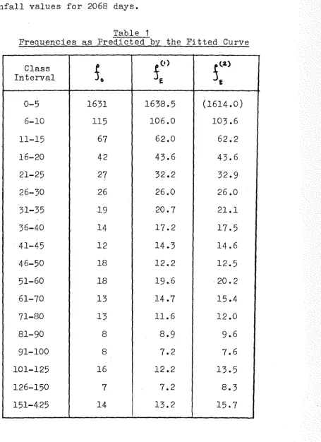
As a numerical example we give in Table 1 Sydney
rainfall values for 2068 days.
Table 1
Frequencies as Predicted by the Fitted Curve
Glass
t
5(1) 5(~)Interval E
E
0-5 1631 1638.5 (1614.0)
6-10 115 106.0 103.6
11-15 67 62.0 62.2
16-20 42 43.6 43.6
21-25 27 32.2 32.9
26-30 26 26.0 26.0
31-35 19 20.7 21.1
36-40 14 17.2 17.5
41-45 12 14.3 14.6
46-50 18 12.2 12.5
51-60 18 19.6 20.2
61-70 13 14.7 15.4
71-80 13 11.6 12.0
81-90 8 8.9 9.6
91-100 8 7.2 7.6
101-125 16 12.2 13.5
126-150 7 7.2 8.3
151-425 14
I
13.2 15.7 [image:17.632.60.516.104.731.2]f'A-
K
and (10) we take
b::
5
and consequently we have '\'\:: Ie;!I •....
L
'X..: ::16 sql
,
r.
....
~~.:::
13'13.11'7i :" \'::.1
Substituting these values in (9) and (10) we find that
equation (9) reduces to f..I.:: o· I~~l.J k.
(10) reduces to
and equation
Solving these equations we get
K::
0·/05 ) p..:: 0·013correct to three places of decimals.
Now for these values of IA) I-<. and ~ we have
b
)(.-1~ e.x..rf""'X.)~
ci'x. ::11·14
~
I<. ::I<. 11·30 .
•
The calculation of the expected frequencies for testing
the goodness of fit is shown in the table. Since
the
?L
1 test is used for testing goodness of fit, theobservations are grouped into classes so that the
expect-ed frequency in any class is not less than 5. To
calcu-late the expected frequencies we use tables of the
incom-plete r-function (Pearson 1922) making a double linear
interpolation, which is sufficiently accurate for our
10
The results are shown in Table 1. The first col-'
umn gives the class interval, the column headed
So
gives the corresponding observed class frequencies. The column(.)
headed
J
gives the expected frequencies. Thus for15
E
degrees of freedom the total
X~
is found to be 7.8, which shows that the fit is an extremely good one.3. Fitting of Truncated Curve Ignoring the
Observations in the Truncated Part
Here we fit a truncated type III curve to the
ob-servations which are all greater than
£
and ignore allobservations which are less than ~
density in this case is given by
• The probabili ty
The logarithm of the likelihood function is given by
L "'-
~ ~ ("><1,ll2.>"· ;1( ... )= 'l'l\k.~'"'" -~~rCI()-lYI<;(1)..)1\)-' " .... I
- J-l L ~i. 0\- 0<·-1) ~
A..-..,
lC4 Ji~1 \':.,
From (11) we obtain the following likelihood
t
0).. _
.!i. _
~
-
.1.i
X .. = 0 Jequations: Q!l)
_ - - lAo ~,.. m , ••
M
oJ'".
1.
"al. _ ,_ .... _
~
'-\(IC.) -~
~l..
i
~~
"IYI ?J~
-
-J'- ~ ""'J ... 'M , ..::: 0 . (I~)
For these equations
~
IL~i.
,
andL
~~.
have the samevalues as before and 'Mdfb7. Equations (12) and (13)
are generally too complicated to be solved. But we can,
however, find approximate solutions and then improve
these solutions to any desired degree of accuracy. Thus
if
f4:.
~o and ~=I<o are an approximate solution for the equations (12) and (13) a better approximatesolu-tion is obtained by taking fJ-= t"'o+£~o I 1<: \<"-\-~I<,,
where
$
,","0 ) ~ 1<" are given by the following equations:(IS)
In this particular example we took
1<=
0.10and ~::: 0.0 \ as the approximate solution for
equa-tions (12) and (13): then with, the help of equations
(14) and (15) we found K= O-ioS and lAo'" O·OI,t correct to three places of decimaL The Newton-Gregory formula was
'Oq
c?q
'0<;
"O'lq
1.2the ~) ~ ... ) ~ I '"21'1\. 'L
'O'l.r:
and ':S
(j,....'O'oC.
etc., which occur in the solutions of equations (14) and
(15). In this case, the approximation previously given
for the integral in G is not sufficiently accurate. The
expected frequencies are given in Table 1 in the column
it:\.)
headed J • The fit of the observed frequencies to the E
expected values, ignoring the interval
lO)
~) givesa
~~~
8-47 which shows that the fit is a good one.The expected frequency in the interval
(0
Ib)
aspredicted by this fitted distribution is 1614. To test
whether this is significantly different from the observed
frequency in this interval we use the following statistic:
E
=
N, - Np
IJ
N~cy ~
V
tt.Jt)where
N,
stands for the number observed in the range(O,b)
J
N
stands for the number of observations in the whole sample, andt
is the probability of an observation falling in the range to)~) given byk.
S
\(.-1L
r
-e.lL\l (-
po. ')lY)L~:)l
-rCI<)
J
Now according to our notation
~(l-~)"" ~(~)\(.).
_ cy. _
'0<;1
~
+
~~.
-
\-P
- ~u... u~U r
-For finding variance and ·covariances of I-L and I< we have
l-ECi"-~
l'd'-L0
-I[ VC><l
""'(>"kl,
'Of.\. .. - E-a ...
al<-E(:~)
(~~
eo.v
(f..l, \1..) V(k) - E Cr~'" )l~1 '1'1-Lj)WI
~"')MJ
'
0- 0006-':''']
-m-l-8'1-~) In
Q
4':'»YI\ - 0- oo:!.7 0- 0'\.:1.'1WI
-n;-from which we get
V
(~)"
o.:.:r!.'l
=
0- 001\'M
Thus we find
t
=
0 -~4 which gives no evidence of acon-centration of probability at zero.
The distribution of mean rainfall based on 94 years
from this type III population is given by
l
e,z)
=
l\k. n\(.-I
l'nf..l.)
~(-nt-tx.)x
r
(11.1<)
'1-870 IS- 870
0-
1.:1.8)
e.Xf(-'_/~8;(Jx:
_
14
1-It corresponds approximately to a:x. distribution wi th
AO
d.f. with skewnessThus the distribution of the mean of 94 observations is
far from normal and a test of significance of such a mean,
Chapter 2
THE FITTING OF A TRUNCATED LOG-NORMAL
CURVE TO DAILY RAINFALL DATA
1. Introduction
In the previous chapter we have discussed a problem
of curve fitting which arose in testing the hypothesis
pro-posed by Bowen concerning the daily rainfall data. A type
III probability distribution of the form
f
~
K
-
f4.'X. k-IJ
(x.) ::
r
(K)e.
?tprovided a good fit to this data. It is more usual, however,
in meteorological practice to fit a log-normal curve of the
type
to rainfall data of this sort.
The first attempt to fit a normal distribution to the
logarithms of the values of a meteorological element appears
to have been made by Blackhouse (1891). He compared the
frequencies of annual rainfall amounts and of their logarithms
16
not very convincing, perhaps because only 30 observations
(1860-89) were available. More recently Brooks and
Car-ruthers (1953, p.102) suggest that a log-normal curve will
give a good fit for any distribution which is positively
skew and leptokurtic. They fitted a log-normal curve to
the rainfall totals at Camden Square, London, for sets of
four consecutive months, between 1870 and 1943, and found
the fit to be good. In their data the frequency rises
quickly to a maximum and then gradually drops down to low
values
The distribution of rainfall data for Sydney
though slightly leptokurtic, is J shaped and therefore
differs from their data. It seems to be quite commonly
be-lieved by meteorologists, however, that the log-normal
curve is generally appropriate for rainfall data. In this
paper we fit a log-normal curve to the Sydney rainfall
data in order to see how good or bad the fit is when
com-pared with that obtained by the use of the type III curve.
To apply maximum likelihood method it is again necessary
to truncate the distribution to avoid the zero values.
Maximum likelihood equations were complicated for the type
2. Fitting of a truncated log-normal curve
The log-normal probability density function is of
the form
in this case we know the origin of our distribution and so
take 0..:0
We now choose a small interval
lo,
J..)
and truncate the distribution at "- , ignoring the actual values of Xless than ~ ,but using the fact that their total number
is known. Thus if ~ be the number of observations
fall-ing in
lo, .{) ,
the rest (1'1-'11"rn)
of the observations willall be greater than 0( •
where XI) "lll.) • • . ) x", //0(
The maximum likelihood equations are given by
""
~
.... "'t\~
-TL,.
~ l~~
-t-"-) :: () ,
(I)a
f.A. Cr """ 6" v:. \(~)
where
fA-
and6
are now no longer population parameters,but, for simplicity, stand for their estimates.
Now
18
After changing the variables in the numerator and
integra-ting by parts, this reduces to
]further
-~Kfl-~~~~-~)J
l:k
~)t.\ll-ir~~ll-t4t}.t.~
o
\
-
--~
(:~)
Which may be similarly reduced to
r~
e.x..pi-a ..
~ll-~)1.} ot~
o
From (3) and (4) we see that
(5)
Using (5) we re-write the likelihood equations
(1)
and (2)as
(G)
'"
'-"rItJ-,o(_~,o~
_~+_\ ~I~~_I"'-)=o
(5"("""J ) - ~ ()~ L_'\
O/"'-
(7)
Now multiplying (6) by
~(~.(_~)
, and subtracting (7)from the result we find
which can be written as
i
~Xi.)~- fJ.:..~rI. €I~X{.
-+
~~o(
20
Thus equations (6) and (8) can be taken as the likelihood
equations for estimating,..,.. and
6' •
To make a comparison with our fitting in Chapter 1 we take
J..
=.5.5 .
From the data we obtain'tY\=4~'"
)
L
'"
~)li.=
1?l'l~.1l1'i3 )i .. '
Substituting these values in (6) and (8), we find that (8)
reduces to
6'~
=
5.l.j~80'7
-(,.'i~ "~ct)
... )
('I)and (6) reduces to
(/0)
Solving (9) and (10) we find ft.=-O·'7and
6:
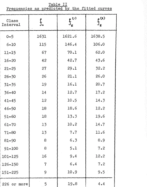
~·38 correct to two places of decimals.The calculation of the expected frequencies for
testing the goodness of fit is shown in table II below.
Since the Chi-square test is used for testing goodness of fit, the observations are grouped into classes so that the
expected frequency in any class is not less than 5. To
<facilitate comparison we have here grouped the observations
into the same classes as we did in Chapter 1 for fitting a
truncated type III distribution.
We
have used the tablesThe results are shown in table II. The first
col-umn gives the class interval, the colcol-umn headed
fo
gives the corresponding observed class frequencies, and thecol-0)
umn headed
Sf
gives the expected frequencies based on log-normal distribution. Thus for 16 degrees of freedomthe total
Jl~
is found to be 44.0, which shows that the fitis a very poor one. On the other hand the column
head-la)
ed
j
gives the frequencies expected on the basis of a£
truncated type III curve, The value of :(1 is here found
22
Table II
Frequencies as predicted by the fitted curves
I
f')
5
(0 )I
Class
So
II
IntervalI
e
e
I
0-5 1631 1621.6 1638.5I
I
6-10 115 146.4 106.0I
I
11-15 67 70.1 62.016-20 42 42.7 43.6
21-25 27 29.1 32.2
26-30 26 21.1 26.0
31-35 19 16.1 20.7
36-40 14 12.7 17 .2
41-45 12 10.5 14.3
46-50 18 18.6 12.2
51-60 18 13.3 19.6
61-70 13 10.2 14.7
71-80 13 7.7 11.6
81-90 8 6.3 8.9
91-100 8 5.1 7.2
101-125 16 9.4 12.2
126-150 7 6.4 7.2
151-225 9 10.9 9.5
[image:31.638.39.509.77.672.2]Finney (1941) showed that if the variable ~ is such that log ~ is normally distributed with meanS and
~ $+L~~
variance 6" then the x. population has the mean
e ..
~tT~('a. 6'"~ )
and variance
e.
e _ \
.
Accordingly the estimates of the mean and standard error of the daily rainfalldis-tribution based on log-normal curve are given by
Mean
=
14.4 and standard deviation=
246.2Based on type III curve these estimates are
Mean = 8.1 and standard deviation
=
24.9But calculating directly from the sample we get
sample mean
=
8.4 and sample standard deviation=
27.9 Thus the mean and standard deviation calculateddi-rectly from the sample agree well with those estimated on
the basis of the type III curve, but deviate considerably
from those estimated on the basis of the log-normal curve.
As is evident from the table this is due to the fact that
the frequency towards the upper tail of the log-normal
curve is very much higher than that observed. This has
re-sulted in increasing the mean, and more especially, the
standard deviation.
On the basis of these results, it would seem that,
at any rate when a certain proportion of days have zero
rain-fall, the better curve to use in fitting rainfall data is the
type III curve, not the log-normal, as has been previously
Chapter 3
THE NUMERICAL EVALUATION OF A CLASS OF INTEGRALS
,1. Introduction
In chapter 2, (page 22, table II) we had occasion
to evaluate the univariate normal integral
-to. .
l')"
N
r
e.x.p5-LJ~~_,...)1J<i"'-J
e .[iii~
J
1.
,E;
N
=Frr
t,
X
..
~ e..~
C:-t~)
aU:
}.,
24
where
AJ
andA1
have specified values depending upon known quantities such as the end points of the class intervals,f-and ~ • These integrals have been studied in detail, but the evaluation of similar normal integrals in more than one
variate present several difficulties. In order to find
whether it is possible to devise a method for numerically
evaluating such normal integrals we take up for consideration
the integral
~
I
=
r···,
of.
"tf'
J
j
('lI."Xa.) ....
'')(111) tAx.,d.X
1 • .. cl?c'tJ )I(.
where Xl ,;(~, .' .. );it.N are jointly distributed in a mul ti-"
variate normal distribution
r(x."x..,···
,X~) with[P
il
1
asthe correlation matrix. The integral has been expressed
in an infinite series of tetrachoric functions for '" )/,2 .
The infinite series is not only complicated, but also is
very slowly convergent and is consequently not of much
practical use. Plackett (1954) obtains a reduction
form-ula for expressing normal integrals in four variates as a
finite sum of Single integrals of tabulated functions.
These integrals have then to be evaluated by a rather
awk-ward numerical quadrature.
In the present chapter ",e first take up the
bivar-iate case and following the method previously described by
Moran (1956), we express
I
as a single integral for whichnumerical integration is not only very easy, but also
ex-tremely accurate as will appear from the numerical examples.
This is shown in Section 2. We discuss the magnitude of the
error of the numerical integration in the bivariate case and
add a few numerical examples in Section 3. We take up the
general case and then show that the method is also easily
applicable to the case of three variables provided the three
correlations satisfy the conditions specified in Section 4.
In Section 5 we devise a method by which we can approximate
the univariate probability integral in terms of a series of
calculat-26
ing bivariate and trivariate probability integrals. The
univariate case leads to a new and interesting set of
in-equalities shown in Section 6.
2. Bivariate case
Write
Let
Now
4 )
J
-I
ex.)::
f"i.1r
V'
J:: )
~
,?(a._~.-tJ.l) ~~ (:~)ch
..-V'
-, ( t.
(eVhr-j'l~+'. ~
('j,.o.,,,+L.tj\x
J
~
(!t1l)
t" )
~.
)
'TL
1
~
,-.
l..l
where
and
Cl...,..
a-
1< ::
Taking ~;; Q2.:: 0.. , we get
1< :
when
r
is positive.(We take
a..:: -
~2.. '" 0.. ,whenr
is negative)Gi ven
r)
~ and \(..i ct)1..,
and 1...2,. are uniquely determin-ed. Having determineda.)
to.
and ~L we replaceJ
by the sumJ::
-h
i
.Q..X-f(-l-t2.rp~'I\~+.I.,)'P(±a.'I\~
;-t2.) ,
"II = -11'
plus sign being taken when
P
is positive and minus sign3. Discussion of error
We now have to consider the magnitude of the
error resulting from replacing the integral
J
by asum.
Goodwin
(1949)
has shown that if we writeIf> V>
S
~x.~(:-x~,)5C:~,)clx.
=
-t.
~
....
1C.'I'Il-.)~>4't-:""'~)
-EC .... )
-1>"
then E(~)is approximately
...
:t
~4>(- ~~)
I
Q..~(:"j"):! (~- ~)~
-"It'
provided ~C.~) is an even function.
.".
mi tted in replacing
5
e..lL~
(_-x.1.)
ol'lL-'t/'
is of the order
Now consider the integral 1>"
Thus the error com-Y'
by ~
L
~(--l ...
2.)
-'"
I
=
J
ex.f1-c."t+f,l}ot~ =~ f",€.lLPt-(~+f,)!J
-
EC~)
-~...,.. -rI'
I
~
t
t )
~
t-
(~+.)}<'-
+
b
j-
("-')'}~1
}
"1f
:: -ex.-pC:
~Il)
S
~
~h
..
€-q
(-x"-)obt
_"11'
"-=~.ffi ~ ;~ e.~ C-~
.. )·
2-Thus
~
fif
~x.f
t
~~
)
is a reasOnable estimate of the upperbound to the error when ~ is not too large.
Consequently an upper bound to the error in replac-11'
ing an integral of the form
S
e.x.ri;(.'X.-t-4tJ
a.
x.
by a sum is of-'"
the same order as the upper bound to the error for the
in-'If'
tegral
S
€'-l<.f
C:-1<'X,2.)cl?L given by-v
...
-h ; ...
I(,~c:-)\'L-e;-k)
-
J:~t\(X.'L)sl~
11'
::: _L.S
~ ~
1:
~X.f0"1\
2.-e...2.x) -
5
~
t-
IC.x.')
cA.(JI<
~
}
.JK
l
-....
-""
'If'
=
..L.) {..'
i.
e.x:1' (-
",'l. ••e/) _ ~
€..)(.p (:-x.'L)
~
1\. }and is approxima::l y equal to
~ l!~2..
e.x..t'
C-1t'!::) .
Thus taking
I ::
1
~t_)«:K.T4)jol.X.and
a::
~ ~\7" ~i-K("'-k+t.)j
we find
i '::
t;.G
when
t.
large.
2-where
le I
<.!1.
ex'p(-.Jk
)exceptNow consider
cr
as given by the integral (2)Thus if
S,-
is the sum replacing12.
then
Consequently if
S,3
is the sum replacingJ
we have-I
$,3
J
=
ITa
30
where
f)
satisfies (3). The fact that the outer integralin (2) introduces a certain averaging effect in kwill
re-sult in the true error being somewhat smaller than this.
We give here a few numerical examples which shows
that the method yields extremely accurate results. We
re-place
J
by a sum over the values of X '" 0, ± 0.5, ± 1.0etc. Taking
r
= 0.5 and.f..-=K ..
;C we get 0.004053 as anesti-mate of
I
which tallies with the tabular value correct tosix decimal places. For error we get
\el ("
0.000004.which is the same as that from the table and
lei
in this· case remains less than 0.000104. Takingr
= 0.2)-t..
= 0.1and K = 0.2 our estimate of
I
is 0.224922 which agrees -10wi th the tabular value and
lei
<.
10 • In all these above examples where we have replacedJ
by a sum over thevalues X= 0, ±o·5. ±. 1·0 etc, we have obtained our estimate
of
I
by summing only 13 terms of the sum forJ.
If we take 0.25 as the interval of summation instead of 0.5, 191-IS
remains less than
10
in all the above examples. As a further example takingf
= 0.8,-k
=
0.8 and I< = 0.3 our estimate ofI
is 0.184795. but that found from the tableis 0.184786. Here
\91
is<.
0.02499. But by replacing by a sum over the values X=
0,±
0.25,±
0.50 etc the estimate is found to be 0.184787 with\91
<.
0.00000005.the discrepancy being due to rounding off.
4. N-Variate case
Under certain conditions to be stated precisely
below, it is possible to evaluate numerically the
N-vari-ate normal integral by expressing it as a K-fold
1I<.
~N)
integral of tabulated functions and then replacing the
where
Consider the integral
I
=
'P~.
t
u.,
")/0..:; i"'}1}'" ...J
~ V
r=.
'==:=
f ...
~
0.)( P Lt
~ L~
\!1
cH:!
hn
L~)
j
1
J
0.., 1I.1f
\l.
stands for the column vector \~
whose ele-32ments have an N-variate joint normal distributions with
zero means and unit variances and
IN
as the variance-covariance matrix.Let X and
~
stand for the column vectors\t}
and(~)
whose elements are independently and normally distributed with zero means and unit variances.It is possible to express ~ as follows:
U
==X -
i?>",
Z
where
Bk.
is anNy-
\<, matrix wi th elements ~'j,
providedLtJ ":
admits real solutions for
t~
In this case
•
I ::
-p~
1
u.~
4-
Q~
j i.ool} 2.}' .. N1
"::.
'?~ ~
'Xi.. )/£ti. +i
J.'
jZi
j i.;I}2..}···N}
1.
J~'"'" "II'
=
I
) ... , )
TIN
~)
Qc
-ti
4'J'
z.}
~)f
In(':'J.i
rz)cL~
(:1.1f)%
.
':t'
l.
F'~
- ,"-.t. - -
-~ \':t
-where
\
To see under what conditions equation (4) admits
of real solution for
i.:
j '" we notice that the right handside of (4) involves NI<. distinct A..:j'J> whereas the left
hand side has
NC
distinctt.'".
In order that1.. .. /}"
2.. ~J
may have real solutions it is necessary that
NC
<
N\(
~.e
2. ... )
Consequently we cannot take \( (,
N-\
unless ther .. '
j)2- ~J
satisfy some further relations amongst themselves. Even
when we take K":: N-I it might not be possible to solve for
2.
the
Ao
ij' /:>taking K::: I
for all the values of
f..'}".
For example by\J
in the trivariate case, we find for
k.;:/J;
the equation.eo,
t
~I l'tt,'2..
)., t.2..
L :: I
-T
"B:B,
.t., t
1- \.,,).::
1.J.1.~
3
(5)
t,
l.~I. ..
t~
lott;-From (5) we get
k
j
J..
tj
t·
t·
~
t
Q-t
ti)
G+
t.n}~
\. :.l (C;)
where
34
From (6) we get
p..
F.:
\<.t"l..
ft. ..
'I... (7)I'l.J _ ,
=
Ij
I<. -l'tt.,
It is evident from (7) that we can reduce the
tri-variate normal integral to a single integral and hence
evaluate numerically by our method if the correlations
r.,.
I PI~ and ~3 are such that their joint product ispositive and each one is numerically greater than the
pro-duct of the other two.
5. Univariate case
The integral
i
..,
e.x.f
t-t
t, . }
(!-t~")
cA.'ll}'" I ;-"X.
~
'!;/'
=
Ji:1\'
1
~~ C-:k?l.~
ch . .
t
(8)
(see Bromwich (1931)
p.388).
As a numerical example we take t
=
1 and replace the right. If'
hand side in (9) by the sum
S
=
t
Cllt)~l:
2'
C.~)
over the()
.... eO.
t '1\2.-1..2.values of x
=
0, + 0.25, ~ 0.50 etc. By taking g(l) and g(nh) correct to 8 decimal places we get 0.15865524 as ourestimate whereas the tabulated value is 0.15865525.
It is easy to obtain a result similar to (9) for
bivariate intefrals, but the method is probably less
satis-factory for computing the double integral because a double
sum is required.
We can now find an upper bound to the error
result-ing from replacresult-ing the integral (9) by a sum. Leaving out
a constant multiplier the integral in (9) to be replaced by
S
."
e-x..p
c.-~
X"") ... _ .
a sum is <II. "
-_"p
p-
1-')t 2.Let
CJO)
To find the error we integrate
(t.2.-tX.2.)1
1-e.xl'
C:-2~~}
round
the rectangular contour wi th vertices ±~1:.
sr .
The poles±it ~
of the integrand arehon the imaginary axis and h, 2h, 3h,
etc., on the real axis.
The residue at any point x
=
nh is-h
e.x.p C:-
~
"l'\2..e,.2)
(the integrals over the vertical parts of the contour
tending to zero).
Now integrating
e.x
t p (-t >e,1")L ... round the rectangular
-t7C.
and is approximately equal to ~
1fUp(~t")
) \_
Cbti.
(ll"t
\1,
-t~ ~)(.t+ ~)J ~p (-t~) ~~. (I~)
-
t
L
~)
J
_~
i::-tl~-
=1)
Since IT
-e.x.\,
i;G.
tj
S c.o.U..
L /-
(rr\~
t)1
j
is an explicit and easilycal-culable expression we could include it in the formula and
!)..JAi!
~x.,?
(-<;
1Tht.
L)regard ~ resulting from the second term in ,r-J~ 'I.. -
't
(13) as the upper bound of the error. For
(9)
this upper bound fot the error reducesand in the numerical case considered above this upper bound
38
6. Inequalities in the Univariate case
By the transformation (8) it
...
is easy to obtainin-equali ties for the integral
r-!..:
S
~
fl')(.1)oI..X,
which are ob-\! 2.1f 7ltained by asymptotic expansion. But by using the sum
re-placing the integral in (9) we can obtain better
inequali-ties for the integral.
b" v
Now
I '"
l
~
V<.f (-
t.
')(.2.)01.. "It '"t't
Lt)j
€.l-.p
tt ')(.
'J
d..
~
.
(4)411\
~ 2:1r t2.-t-x.:I..t -lI'
Now consider the sum
S «9,:
t:<a
It)-t.r
eX'pI-F~t4jlreplacing
I
-J air -'" t2.-\-~+Q.)2.
~tC!l...) is a periodic function of G\. wi th period
.e-.
andsatisfies the relation
In order to determine the absolute extrema of
sea..)
we express
S(a.)
as a Fourier Series of period-t
as follows. Let'r:f :i. m \i
a.
2:
AWI~ -~
~
i
-!
('I4..-to..)J
c{-t'l..
+
("f\.k.-to..) La..·41
As a numerical example we take t = 1.0. Replacing the
integral in (14) by a sum over the values of x
=
0,±
1.0,t
2.0 etc we havesl\)= 0.15679 andS(C)
= 0.16053 whereas 1=
0.158655 correct to six decimal places as found from the table. But by replacing the integral by asum over the values X
=
0,±
0.5,±
1.0 etc wePart II
Chapter 4
ON TESTS OF RANDOMNESS OF POINTS ON A LATTICE
1. Introduction
In this chapter we will be using Pitman's
cri-terion to judge the merits of various tests of
random-ness of the distribution of points on a lattice.
P.V. Krishna Iyer (1949b) has shown that a givsn
distribution of diseased plants in a rectangular
planta-tion can be tested for randomness by comparing either (1)
the number of joins between adjacent diseased plants or
(2) the number of joins between healthy and diseased
plants adjacent to each other, with its expectation for 43
the observed numbers of diseased and healthy plants in the
field. He has discussed two cases: (i) where the
proba-bility of any plant being diseased is the same as that of
any other plant being diseased and independent of the
num-ber of the diseased plants and (ii) where the numnum-ber of
diseased plants is known and interest attaches only to their
distribution over the area. They are called free and
plantation is referred to as a lattice of pOints, with
diseased plants as black points and healthy plants as white
points. One may also use the number of joins between
ad-jacent healthy plants as a test criterion.
In this chapter we shall discuss a rectangular
lattice of points each of which may be of two kinds, say
black or white, and compare the relative merits of the
three tests of randomness. These tests will be based on
the free sampling model. The distribution of these test
statistics involve the unknown parameter
p
(theproba-bility of a point being black on the null hypothesis).
But as the number of black paints provides a sufficient
estimator for
t '
an exact test may be made by takingthe number of black points fixed. The conditional
distri-bution of a test statistic is then free of the unknown
parameter
p
(This technique is similar to thatdis-cussed by Mood (1950) for testing independence in 2 x 2
contingency tables). Tests made in this way are
appropri-ate to the free sampling situation. For this reason, the
procedures and results below apply to tests made in
practice.
Intuitively one feels that if the probability
P
of a point being black is low the number of black-black
jOins will give the best test of the three, while for a
45
In order to verify this conjecture it will be
ned-essary to set up a suitable alternative to randomness. The
problem of the trees in an orchard suggests a two
dimension-al simple Markoff Chain. The difficulties in consistently
formulating such a model have prevented its use and as an
expedient the following alternative to randomness has been
used. We shall assume that black points are first
distri-buted at random on the lattice with probability
fl
andthat the black joins are then distributed, independently
of the original distribution of black points with
proba-bili ty •
We shall be concerned with the asymptotiv
effici-ency of various tests and therefore with probabilities of
contagion which are small (since any reasonable test will
pick up an appreciable departure from the null hypothesis).
The probability of the disease spreading more than once
will then be a small quantity of higher order than one.
The model used corresponds to the impossibility of
contag-ion spreading, from an initial infectcontag-ion, to trees which
are not adjacent. Nevertheless the previous
considera-tions suggest that the asymptotic theory will still be
If the overall probability of a black point
is
P
,we have(' )
We treat
r.
onH,
as a function Of'1 .".f!
tt-
D-l'0~-r~J
is fixed. The kind of situation we have in mind is one
where
f
has been estimated from the observed number ofblack points (relative to the total number of points) and
we wish to know whether
r
is of the form given inHo
or
HI.
One can also have the positionand one wishes to test whether
p::
PI
orwhere
R
is knovm~
\- 0-\>.)6-
p
a)"j,
where p~ is unknown. This situation seems less relevant
to the type of problem met in practice, but will be
mention-ed shortly below.
Moran (1947) has shown that the distribution of the
number of black-white (and therefore black-black or
white-\'ihi te) joins, is asymptotically normal when
Ho
is true.In order to judge the relative merits of the three tests we
shall therefore use Pitman's criterion of the asymptotic
relative efficiency of the two tests (Noether 1955).
Since for this purpose we shall require the
vari-ances of the number of blaCk-white, black-black and
white-white joins as obtained by Moran, we quote below his
47
Let V~ and Vp;,Q, stand for the variances of the
number of black-white and black-black joins respectively.
The results as obtained by Moran for a rectangular 1attice
of Y'nX'Y\.. points with the probabilities? of a point being
b1ack and
tt:.I-,,\,
of a point being white are given by1.. 'l.r,
4 : \
(
V~
':
~'por(S)'/ll\-.,m-'1l\-4) ~4
'pI\-
\.\'?I)'/I..,\~n-I
Y11Y1-9) I :I.)V~(l,
_
l~Y't\n-m-Y\)~ ~~~mY\-\'l.m-\'-'\'\
-Tit)\>a-+~
-+~~)'/I-+
\'?In - \4\\\l\ -i)
'p(a)
Replacing \' by
Oy-
in the expression forViti\!)
we a1so have the variance of the number of white-white joins as:b
Vww _
(~"/I\Y\-lY\-"I\)~
-+
(\1.mn
_I'-'M-I'-'t\-\-a-)'\--T
...
2. Pitman's Criterion
Here we give a brief summary of the Pitman's
cri-terion as discussed by Noether. Consider two tests based
on the statistics
'1;"and
~"to
test the null hypothesis\(
Ho··
&=
&0
against the alternativeHI:
6=6,,=6 ..
-ton"
where
I,
is an arbitrary positive constant. If the twotests have the same size, it is reasonable to define the
asymptotic relative efficiency of the second test
proced-ure with respect to
of the ratio 111
the first test procedure as the limit
)\2.
, where 1I~ is the sample size of the
second test required to achieve the same power as the
first when using a sample of size ~I with respect to a
given alternative.
Under certain general conditions the ratio is
given by
lJn) [
np:l\te~2~e.)J ~'O
'l'I1
-
04-'1'\-\'11'-
..L
'1\2-l
~
)
~,,(
0·)/61"(
eo)]
1>\ Swhere for
" =
I):t
E
Cll,,)
~
'\¥i'tl(
6 )
I~
49
I\U 1&)
is the first derivative off\\'\",.\6)
which does .."f ill\. "
not vanish for
e::
6.
andb
satisfies the relation-'I'll'''''' .)/
~'\1'
"t\"",>\(e~6"lILe.):-
Ci. 7
0301'
some ~~oIn most of the cases 111:: I and
S::
~3. The asymptotic efficiency of the tests
For a finite lattice of points the overall
proba-bility of a point being black under the alternative
hypoth-esis will have the
valUeSt,-(I-P,)Q-I'2.)'"! )
i,-(l-p,)O-~~5'}
or
1
\-
(l-p,)O-I'~yI1
according as the point is a corner, a border or an internal pOint. Asymptotically, however, theborder and corner points may be neglected. This is
tanta-mount to supposing our observed lattice as a subdomain of a
larger lattice. We shall use the probability under H.given
above as the probability of a point being black irrespective
of its position.
Thus the probability of a black-white join under the
alternative hypothesis is
(S")
and that of a white-white join is
eubtracting the sum of (5) and (6) from unity we find that
the probability of a black-black join is
1_
~
(I-P2.)!jQ-l>I)+
(H>2.)'1Q-p.l .
('1)I f we let
'PI::'
P )
a=
0 and I-PI =c.y.
in (5), (6) and(7), they reduce to ~\"
cv-)
0.,.2.
andfA. ,
which are theprobabilities of a black-white, white-white and black-black
join respectively on
Ho .
Denoting the expected number of black-white joins
by
~
we have under the alternative hypothesis~
-= :.
(:J.l"I\Y\ --m-lI)
0-
1"2.)
~(I-P.)
1
\-
Q-r.lO-PI)}
Jwhich by the relation in equation (1) reduces to
For the number of black-black joins we have similarly
~lj
=
(?"nI"I'I-
m-n)
11-:1.
(1-1>$0-1>.)-+
o-t>1)'TC
I- p
,iJ
CIr.1. "\
=
~m'l\-
m-'l'I)
(1-
:~
+
1-1'..)'
Denoting the asymptotic efficiency of the test based on
black-51
t
't~
C
!l.l'YIl'l-'m-lI)1}1(~n"l-l'YI-lI)
p \ 0"l'nn-l:ll'Yl-lll1t8)p
3-t (13111-1 !:!...,-14l'Y1t1-S)>'tl4
.
::
~1~
1
a'P'Y'(h
n-'1
m-'111+'t)+4P"r'i..(l?llYl+\SlI-14l'n1l-i)}l~
(2"MlI--m-lIYJ
p+
11"2--
:;._ '1),+
1p
'l.In calculating the relative efficiency
p
is treatedas "'- constant and
h.
as a variable.Consequently the test based on black-\~hi te joins
is more, equally or less efficient than the test based on
black-black joins according as
"fl+'1p2-_
:I.. -
'11>
-to <"/l'
2..is greater
than, equal to or less than unity, that is according as~
is greater than, equal to or less than
:!r .
By symmetry the following asymptotic relative
asymptotically the most efficient test therefore is the
test based on the number of black-black joins when 0 (I'{ ~ ,
on the number of black-white joins when ~~
\>!,
~ or on the number of whi te-whi te joins for ~ ~ \' <. \ •'T
The same results will be ohtained if a three
dimen-sional lattice of ..tXWl)(''YI. points is considered.
In the alternative case where
1',
is known and one wishes to test whetherf=h
or1>
= 1- (I-I'I)O-I'.)'tthe number of black points may also be used as a test
cri-terion. Taking this as well as other tests into
considera-tion we find that the test based on black-black joins is
Chapter 5
STATISTICAL ANALYSIS OF AUSTRALIAN
PRESSURE
DATA1. Introduction
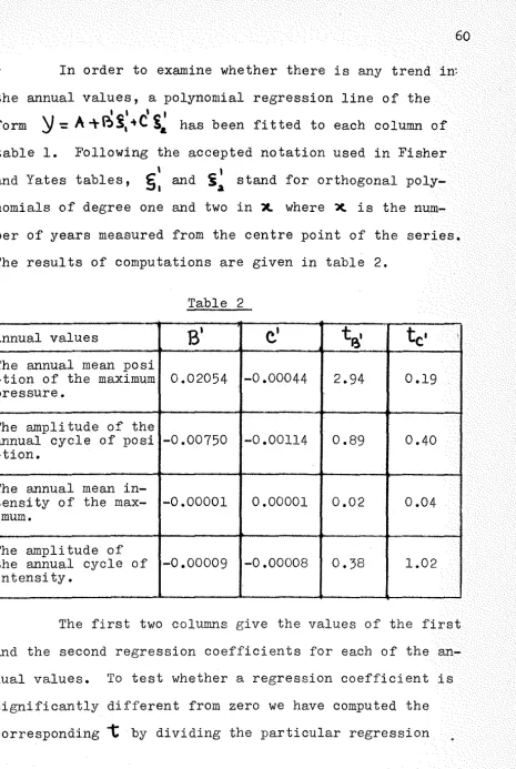
53
In this chapter we consider the statistical
analy-sis of Australian pressure data in order to test the
fol-lowing hypothesis which arose out of Deacon's (1953) work.
Deacon compared the mean daily maximum temperatures for the
summer seasons between two 30 year periods 1881-1910 and
1911-1940 for some Australian inland localities. Table 1
of his paper gives temperature differences for the two
periods for 14 stations. All these show a consistently
lower temperature in period 2 than in period 1. He also
found that for the period 1911-1950, the summer rainfall
over much of the southern part of Australia was considerably
greater than in the previous 30 years. He conjectured that
these changes were due to a climatic trend and by noting the
difference in the character of the annual variation in