Eccentricity-dependent temporal contrast tuning in human visual cortex measured with fMRI.

This is a repository copy of

Eccentricity-dependent temporal contrast tuning in human

visual cortex measured with fMRI.

.

White Rose Research Online URL for this paper:

http://eprints.whiterose.ac.uk/135910/

Version: Published Version

Article:

Himmelberg, Marc Mason orcid.org/0000-0001-9133-7984 and Wade, Alexander Robert

Patrick orcid.org/0000-0003-0656-2664 (2019) Eccentricity-dependent temporal contrast

tuning in human visual cortex measured with fMRI. Neuroimage. pp. 462-474. ISSN

1053-8119

https://doi.org/10.1016/j.neuroimage.2018.09.049

[email protected]

https://eprints.whiterose.ac.uk/

Reuse

This article is distributed under the terms of the Creative Commons Attribution (CC BY) licence. This licence

allows you to distribute, remix, tweak, and build upon the work, even commercially, as long as you credit the

authors for the original work. More information and the full terms of the licence here:

https://creativecommons.org/licenses/

Takedown

If you consider content in White Rose Research Online to be in breach of UK law, please notify us by

measured with fMRI

Marc M. Himmelberg

, Alex R. Wade

a_{Department of Psychology, The University of York, Heslington, York, YO10 5DD, United Kingdom}

b_{York NeuroImaging Centre, The Biocentre, York Science Park, Heslington, York, YO10 5NY, United Kingdom}

A R T I C L E I N F O

Keywords: Visual cortex

Temporal contrast sensitivity Magnocellular pathway Eccentricity fMRI

Population receptivefields

A B S T R A C T

Cells in the peripheral retina tend to have higher contrast sensitivity and respond at higherflicker frequencies than those closer to the fovea. Although this predicts increased behavioural temporal contrast sensitivity in the peripheral visualfield, this effect is rarely observed in psychophysical experiments. It is unknown how temporal contrast sensitivity is represented across eccentricity within cortical visualfield maps and whether such sensi-tivities reflect the response properties of retinal cells or psychophysical sensitivities. Here, we used functional magnetic resonance imaging (fMRI) to measure contrast sensitivity profiles at four temporal frequencies infive retinotopically-defined visual areas. We also measured population receptivefield (pRF) parameters (polar angle, eccentricity, and size) in the same areas. Overall contrast sensitivity, independent of pRF parameters, peaked at 10 Hz in all visual areas. In V1, V2, V3, and V3a, peripherally-tuned voxels had higher contrast sensitivity at a high temporal frequency (20 Hz), while hV4 more closely reflected behavioural sensitivity profiles. We conclude that our data reflect a cortical representation of the increased peripheral temporal contrast sensitivity that is already present in the retina and that this bias must be compensated later in the cortical visual pathway.

1. Introduction

There is a mismatch between electrophysiological retinal measure-ments and psychophysical measuremeasure-ments of temporal contrast sensitivity across the visual field. Eccentricity-dependent differences in retinal temporal sensitivity originate in the cone photoreceptors–peripheral cones respond faster and are more sensitive toflicker when compared to those in the fovea (Sinha et al., 2017). These signals arefiltered through the retinal ganglion cells (RGCs), where there is an increase in the pro-portion of parasol to midget RGCs with increasing retinal eccentricity (Connolly and van Essen, 1984;Dacey, 1993,1994;Dacey and Petersen, 1992;De Monasterio and Gouras, 1975). Temporal frequency sensitivity is thought to be related to the relative activity of parasol to midget RGC populations which form the magnocellular and parvocellular pathway, respectively (Hammett et al., 2000;Harris, 1980). On average, RGCs in the periphery have larger receptivefields and cells with such receptive

fields have increased contrast sensitivity (Dacey and Petersen, 1992;

Enroth-Cugell and Shapley, 1973). Overall then, the peripheral retina has relatively more parasol cells, those cells integrate from larger portions of the retina, and they are fed by cones with brisker response kinetics (Dacey and Petersen, 1992; Enroth-Cugell and Shapley, 1973; Sinha

et al., 2017). From such physiological differences we might expect sub-jects to be more sensitive to low contrastflickering stimuli in more pe-ripheral regions of the visualfield.

These predictions are not generally confirmed by psychophysical measurements of temporal contrast sensitivity across space. Previous research has found that psychophysical temporal contrast thresholds are approximately independent of visualfield eccentricity (Koenderink et al., 1978;Virsu et al., 1982;Wright and Johnston, 1983). Although such thresholds (which by definition, occur at relatively low contrast) are independent of eccentricity, very low spatial frequencies might be an exception: previous papers report an increase in criticalflicker frequency with increasing eccentricity (Hartmann et al., 1979;Rovamo and Rani-nen, 1984). How these eccentricity-dependent sensitivities to temporal contrast are represented in the visual cortex is currently unknown.

The early visual cortex is organised retinotopically; visual space is mapped topographically, with foveal receptivefields mapped towards the occipital pole and more peripheral receptive fields mapped in increasingly anterior areas of the cortex (Engel et al., 1997). Perhaps then, investigating sensitivity to temporal contrast across cortical space can help to explain the discrepancy between measurements of retinal and psychophysical temporal contrast sensitivity. Previous research has

* Corresponding author.

E-mail address:[email protected](M.M. Himmelberg).

https://doi.org/10.1016/j.neuroimage.2018.09.049

Received 2 May 2018; Received in revised form 10 September 2018; Accepted 18 September 2018 Available online 20 September 2018

found centrally located sustained and peripherally located transient temporal channels in primary visual cortex, and these channels are thought to reflect responses from different classes of cells (Horiguchi et al., 2009). One might ask whether the relative weighting of response properties of peripheral retinal cells to temporal frequency and contrast is maintained in V1 and other early visual areas. One might also ask at what point in the cortical pathway is temporal contrast sensitivityfiltered to reflect psychophysical sensitivity across space, rather than retinal sensi-tivity. One might expect suchfiltering to occur in higher-order visual areas that are typically specialized for complex feature identification computations, and are less reliant on temporal frequency and contrast information.

How do measurements of cortical temporal contrast sensitivity differ across visual space, and how do such cortical sensitivities relate to behaviour? To answer this, we used fMRI to measure voxel contrast response functions (CRFs) at a range of temporal frequencies and plotted responses as a function of pRF eccentricity in different visual areas. Additionally, we obtained psychophysical temporal contrast threshold measurements in central and near-peripheral regions of visual space. Previous research has found that the optimal contrast sensitivity of the primate visual system is approximately 8 Hz, thus we predicted that we would observe a similar peak contrast sensitivity, independent of ec-centricity, in our psychophysical and fMRI data (Hawken et al., 1996;

Kastner et al., 2004;Singh et al., 2000;Venkataraman et al., 2017). Next, due to retinal biases, we predicted that in early visual areas contrast sensitivity would be greater at a high temporal frequency in pRFs rep-resenting more peripheral locations of the visualfield. Conversely, if cortical sensitivities are to shift to be more reflective of behaviour at some point in the visual cortex, it is predicted that such areas will show no difference in temporal contrast sensitivity across pRF eccentricity.

2. Materials and methods

2.1. Participants

Nineteen participants (meanSD age, 27.895.72; 9 males) were recruited from the University of York. All participants had normal or corrected to normal vision. Each participant completed a 1-h psycho-physics session and two 1-h fMRI sessions. In thefirst fMRI session, two high-resolution structural scans and six pRF functional runs were ob-tained. In the second fMRI session, 10 temporal contrast sensitivity (TCS) functional runs were obtained. All participants provided informed con-sent before participating in the study. Experiments were conducted in accordance with the Declaration of Helsinki and the study was approved by the ethics committees at the York NeuroImaging Centre and the University of York Department of Psychology.

2.2. Behavioural psychophysics

2.2.1. Experimental design

To investigate psychophysical temporal contrast sensitivity, we measured contrast detection thresholds for four temporal frequency conditions (1, 5, 10, and 20 Hz) at two eccentricities (2_{and 10). 75%}

correct detection thresholds were obtained using a‘2 Alternative Forced Choice’ (2AFC) method using four randomly interleaved Bayesian staircases in separate eccentricity blocks (Kontsevich and Tyler, 1999). A single block of 200 trials (50 of each temporal frequency condition) was presented at either 2_{or 10from centralfixation on the temporal visual}

field meridian. Participants were instructed to maintainfixation on a central cross and to respond, via keyboard press, whether the stimulus grating appeared on the left or right of fixation. Participants were informed via a toned‘beep’if their response was correct or incorrect. These responses were recorded using Psykinematix software (KyberVi-sion, Montreal, Canada, psykinematix.com). After each response, a separate toned‘beep’was presented in conjunction with the fixation crossed briefly changing to ‘o’then back to ‘x’ to signify the onset

succeeding trial, which then began 500 ms later. Thefirst 10 trials were practice and not included in the analysis. The temporal frequency of the stimulus was randomized within each block. Participants completed each eccentricity condition block four times and responses were fit with Weibull functions of stimulus contrast. This resulted in four 75% contrast detection thresholds for each temporal frequency and eccentricity com-bination. For each condition, the average of these 4 thresholds was the

final threshold.

2.2.2. Stimuli

Psychophysical stimuli (seeFig. 1) were designed using Psykinematix software and were presented on a NEC MultiSync 200 CRT monitor running at 120 Hz. Gamma correction was performed using a‘ Spyder5-Pro’ (Datacolor, NJ, USA) display calibrator. Stimuli were circularly windowed sine wave gratings outlined with thin white circles to elimi-nate spatial uncertainty (Pelli, 1985). Grating spatial frequency was set to 1 cycle per degree (cpd) and were presented for 500 ms. At 2

eccen-tricity, the grating had a 0.5 _{radius. Using M-scaling to account for}

cortical magnification, at 10 _{eccentricity the stimulus had a 1.021}

radius (Rovamo and Virsu, 1979).

2.3. Functional neuroimaging

2.3.1. fMRI stimulus display

Stimuli were presented in the scanner using an PROpixx DLP LED projector (VPixx Technologies Inc., Saint-Bruno-de-Montarvile, QC, Canada) with a long throw lens that projected the image through the waveguide behind the scanner bore and onto an acrylic screen. The image presented had a resolution of 19201080 and a refresh rate of 120 Hz. Participants viewed this screen at a viewing distance of 57 cm using a mirror within the scanner. Gamma correction was performed using a customized MR-safe ‘Spyder4’ (Datacolor, NJ, USA) display calibrator.

2.3.2. fMRI data acquisition

Scans were completed on a GE Healthcare 3 T Sigma HDx Excite scanner (GE Healthcare, Milwaukee, WI). Structural scans were obtained using an 8-channel head coil (MRI Devices Corporation, Waukesha, WI) to minimize magneticfield inhomogeneity. Functional scans were ob-tained with a 16-channel posterior head coil (Nova Medical, Wilmington, MA) to increase signal-to-noise in the occipital lobe.

2.3.3. Pre-processing of structural and functional scans

Two high-resolution, T1-weighted full-brain anatomical structural scans were acquired for each participant (TR, 7.8 ms; TE, 3.0 ms; TI, 450 ms; voxel size, 1.31.31 mm3; flip angle, 20_{; matrix size,}

176256 x 257). To improve grey-white matter contrast, the two T1 scans were aligned and then averaged together using FSL tool FLIRT (Jenkinson et al., 2012). This averaged T1 was automatically segmented using a combination of FreeSurfer (http://surfer.nmr.mgh.harvard.edu/) and FSL, and manual corrections were made to the segmentation using ITK-SNAP (http://www.itksnap.org/pmwiki/pmwiki.php) (Teo et al., 1997). At the beginning of each functional session, one 16-channel coil T1-weighted structural scan with the same spatial prescription as the functional scans was acquired to aid in the alignment of functional data to the T1-weighted anatomical structural scan.

Functional data were pre-processed and analysed using MATLAB 2016a (Mathworks, MA) and VISTA software (https://vistalab.stanford. edu/software/) (Vista Lab, Stanford University). Between and within scans motion correction was performed to compensate for any motion artefacts that occurred during the scan session. Any scans with>_{3 mm}

anatomical scan. First, we applied a manual alignment by using landmark points to bring the two volumes into approximate register. Next, we used a robust EM-based registration algorithm as described byNestares and Heeger (2000) to fine tune the alignment. The final alignment was checked by eye to ensure that the automatic registration procedure optimised thefit. This alignment was used as a reference to align our functional data to our full-brain anatomical scan. These functional data were then interpolated to the anatomical segmentation.

2.3.4. Population receptivefield mapping scans

pRF scan sessions consisted of six 6.5-min pRF stimulus presentation runs collected using a standard EPI sequence (TR, 3000 ms; TE, 30 ms; voxel size, 222.5 mm3,flip angle 20_{; matrix size, 9696 x 39).}

Here, a drifting pRF bar stimulus was used to obtain retinotopic maps and estimates of pRF parameters (Dumoulin and Wandell, 2008). A single bar (width 0.5_{) was swept in one of eight directions within a circular}

aperture (10_{radius) with each sweep lasting 48 s. Using the conversion}

of visual angle to retinal eccentricity, 10_{radius corresponds to mapping}

2.83 mm radius retinal space (Drasdo and Fowler, 1974). To stimulate a broad population of neurons, the pRF carrier consisted of pink noise at 5% contrast, where the noise pattern changed at 2 Hz (seeFig. 2). A 12 s (4 TR) dummy run was included at the beginning of each functional run to allow for the scanner magnetization to reach a steady state. To maintainfixation throughout the scan, participants completed an atten-tional task where they responded, via button press, when the orientation of thefixation cross changed. This task was set up so that on average, every 2 s there was a 30% chance of a change in the orientation of the

fixation cross.

Using mrVista, pRF positions (i.e. eccentricity and polar angle pa-rameters) and sizes were estimated for each voxel using the standard pRF model (Dumoulin and Wandell, 2008). InFig. 3we present exemplar eccentricity, polar angle, and pRF size maps from one participant. Following the nomenclature ofWandell et al. (2007)we delineatedfive bilateral regions of interest (ROIs); V1, V2, V3, V3a, and hV4, by hand on corticalflat maps based on polar angle reversals for each participant (see

Fig. 3B).

2.4. Temporal contrast sensitivity (TCS) functional scans

2.4.1. Stimulus

To investigate voxel temporal contrast sensitivity, we presented participants with a vertically oriented contrast reversing sine grating within a circular aperture (10_{radius). The stimulus was generated and}

presented using MATLAB 2016a and Psychtoolbox v.3.0.13 (Brainard, 1997). We modulated both the contrast and temporal frequency of the grating. Within each functional run the sine wave grating was presented at 20 condition combinations of Michelson contrast (1, 4, 8, 16, and 64%) and temporal frequencyflicker (1, 5, 10, and 20 Hz) (Michelson, 1927). The spatial frequency of the grating was held at 1 cpd. Each stimulus condition was presented once per run and lasted 3 s. A baseline condition of mean luminance was presented for 3 s during each run. Here, a single contrast reversal was defined as one complete on-off cycle off the stim-ulus. A visual representation of the experimental design is illustrated in

Fig. 4.

2.4.2. Data acquisition and analysis

TCS functional scan sessions consisted of ten 3.5-min stimulus pre-sentation runs collected using an almost identical EPI sequence to that used for the pRF mapping (TR, 3000 ms; TE, 30 ms; voxel size, 222.5 mm3,flip angle 20_{; matrix size, 9696 x 39). The stimulus}

was presented using an event related design in which condition ordering was randomized within each run. A randomized interstimulus interval separated each condition and was jittered to last on average 6 s. Again, a 12 s (4 TR) dummy run was included at the beginning of each functional run to allow for the scanner magnetization to reach a steady state. Par-ticipants completed the same attentional task as the pRF runs throughout the experiment.

TCS data were analysed using MATLAB 2016a and VISTA software. A general linear model (GLM) was implemented to test the contribution of stimulus condition to the BOLD time course (Friston et al., 1998). We used the default two-gamma Boynton HRF from SPM5 andfit the model to an averaged time course of BOLD signal changed for each stimulus condition by minimizing the sum of squared errors (RSS) between the predicted time series and the measured BOLD response. This resulted in 20 Beta weight estimates for each voxel, reflecting sensitivity to each stimulus condition.

Fig. 1. 2AFC stimulus at two eccentricity conditions. In A) aflickering stimulus grating appears in the right circle at 2_{eccentricity, while in B) theflickering stimulus} grating appears in the right circle at 10_{eccentricity. Participants must select which circle the grating appears in.}

2.5. Statistical analysis

2.5.1. Plotting beta weights as a function of eccentricity and pRF size

Only pRF and TCS voxels with 10% variance explained were retained for further analysis. The pooled total voxel count for each ROI and the total voxels removed for falling below 10% variance explained are presented inTable 1. For each voxel within each participant's ROI, a pRF eccentricity value and a pRF size value was extracted from the pRF data. The same ROIs were then overlaid on each corresponding partici-pants TCS data and 20 beta weights (1 beta weight per stimulus condi-tion) were extracted for each voxel. Thus, each voxel was allocated 22 values: a pRF eccentricity value, a pRF size value, and 20 beta weights reflecting voxel sensitivity to each TCS stimulus condition. Polar angle values were not included in the analysis.

For each participant, beta weights were plotted as a function of pRF

eccentricity; foveal, parafoveal, or peripheral. For each ROI, foveal pRFs were defined as being between 0.2 _{and 3.0 eccentricity, parafoveal}

pRFs were defined as being between 3.0_{and 6.0eccentricity, and}

pe-ripheral pRFs were defined as being between 6.0_{and 10.0eccentricity.}

Visualisation of how these data are partitioned and their correspondence to visual space is illustrated inFig. 5.

pRF size and eccentricity are highly related measures: average pRF sizes increase with eccentricity (Dumoulin and Wandell, 2008). For completeness, we additionally analysed our data as a function of pRF size to complement the eccentricity-based analysis. Each participant's beta weights were plotted as a function of pRF size; small or large. Receptive

field sizes progressively increase as one moves up the visual hierarchy and what constitutes a‘small’or‘large’pRF will differ depending on ROI (Wandell et al., 2007). To account for this, within each ROI,‘small pRFs’

were defined as having a size value between 0.25_{(as a hard minimum)}

and the median pRF size, whilst‘large pRFs’were defined as a size value between the median and the maximum pRF size (with a maximum cut off of 10_{). These normalized pRF sizes are presented in AppendixTable A1}

and the pRF size analysis is presented in the Supplementary Materials.

2.6. Contrast response functions

For each participant's ROIs, hyperbolic ratio functions werefitted at each of the four temporal frequencies for each eccentricity partition of data. We modelled contrast response using the following equation:

R_ðC_{Þ ¼} R0þRmax cn

cn

50þ c

n

Where C is stimulus contrast,R0 is the baseline response,Rmax is the maximum response rate,c50 is the semi saturation contrast, and the exponent, n, is the rate at which changes occur and was held at 2 (Albrecht and Hamilton, 1982;Boynton et al., 1999). This resulted in four contrast response functions (CRFs) per ROI at each eccentricity for each participant (i.e. each participant had four CRFs within V1 foveal, four CRFs within V1 parafoveal, and four CRFs within V1 peripheral).

From each CRF we extracted C50, the contrast semisaturation point. This is the amount of contrast required to elicit half the maximum response of the CRF. A decrease in C50results in a leftward shift in the CRF, indicating thatlesscontrast is required to hit this 50% response, thus, is representative of anincreasein contrast sensitivity (Albrecht and Hamilton, 1982). Illustration of such a shift in C50is presented inFig. 6.

2.7. Analysis - repeated measures ANOVAs

For our psychophysical experiment, we carried out a 4 (temporal

Fig. 3. Exemplar left hemisphere retinotopic maps with ROI border overlays presented onflattened cortical representations for one subject. In A) we present ec-centricity maps in which pRF ecec-centricity increases with distance from the fovea. In B) we present polar angle maps with border overlays based on polar angle re-versals. In C) we present pRF size maps, that show an increase in pRF size within and between ROIs.

Fig. 4. Visual representation of temporal contrast stimulus conditions. The sine wave grating sweeps through 20 temporal contrast conditions, with each con-dition being presented once per run for 3 s.

Table 1

Results of voxel thresholding. Voxels with less than 10% VE in both the pRF and the TCS data are removed from further analysis (N¼19).

ROI Pooled total voxels Pooled voxels under 10% VE Proportion removed

V1 77693 34314 44.16%

V2 76991 32555 42.28%

V3 70977 26907 37.81%

V3a 55659 23235 41.75%

frequency) x 2 (eccentricity) repeated measures ANOVA with 75% contrast detection thresholds as the dependent variable and looked at simple effects to compare between conditions. For our fMRI experiment we ran a 5 (ROI) x 4 (temporal frequency) x 3 (pRF eccentricity) repeated measures ANOVA with C50 as the dependent variable and looked at simple effects analyses to answer our targeted predictions.

2.8. Polynomialfits and bootstrapping

Tofind the temporal frequency at which contrast sensitivity peaks at each eccentricity and within each ROI (or for psychophysics, at the two visualfield locations tested), we used MATLAB function‘bootstrp’ to bootstrap 2000 second order polynomialfits (generated using MATLAB function‘polyfit’) to the means of random permutations of our C50data (fMRI) and contrast detection thresholds (psychophysics). These data were permutated using random sampling (19 draws) with replacement. We then found the mean of the zero points of thefirst derivatives of each of the 2000 second order polynomialfits. This point reflects the average level of temporal frequency at which contrast sensitivity peaks.

3. Results

Our psychophysical data were broadly consistent with those from previous studies indicating little difference in temporal frequency tuning

between fovea and near-periphery, and an overall‘U’shaped temporal frequency threshold tuning function with a minimum contrast threshold (peak sensitivity) around 8 Hz. In our imaging data, we found profound changes in C50as a function of both temporal frequency and pRF ec-centricity. First, we found all visual areas studied had an overall (i.e. ignoring any effects of eccentricity) peak in contrast sensitivity at 10 Hz. Next, in early visual areas we found that pRFs representing the peripheral visualfield had increased contrast sensitivity at a high temporal fre-quency (20 Hz) when compared to pRFs representing the fovea –

consistent with effects predicted from retinal physiology. This difference disappeared in area hV4, where no consistent eccentricity-dependent difference in contrast sensitivity at any temporal frequency could be measured. We fed our 20 Hz C50measurements from all ROIs into a linear model and found that hV4 had the highest contribution to afit of psy-chophysical contrast sensitivity. Overall, wefind that contrast sensitivity in the periphery of V1, V2, V3, and V3a is increased at a high temporal frequency, but this sensitivity is lost in hV4 as cortical tuning becomes more similar that of the psychophysical observer. Here we present a summary of our results for our psychophysical and fMRI data. Supporting pRF size results are available in Supplementary Materials.

3.1. Psychophysical results: contrast sensitivity

A 2 x 4 repeated measures ANOVA was performed to assess whether there was a difference in psychophysical contrast detection thresholds between eccentricity and temporal frequency. Mauchly's test of Sphe-ricity was violated for both the main effect of temporal frequency (χ2(5)¼42.321,p<.001) and the temporal frequency * eccentricity

interaction effect (χ2(5)¼11.619,p¼.041). Thus, a Greenhouse-Geisser

correction was applied to the results of these effects.

The analysis found a significant main effect of temporal frequency (p<_{.001) and a significant eccentricity * temporal frequency interaction}

effect (p<_{.001). F-values and p-values are presented in Appendix}

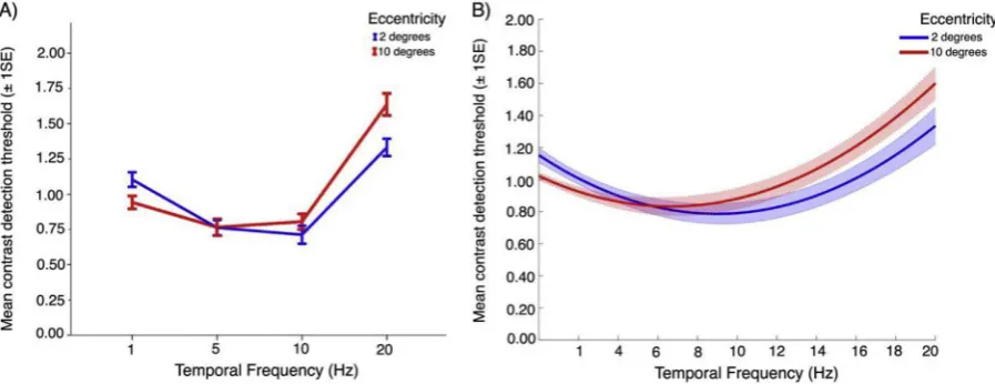
Table A.2. As illustrated inFig. 7A, contrast detection thresholds were higher at 1 Hz when presented at 2_{eccentricity (p<.000). Conversely,}

at 20 Hz, contrast detection thresholds were higher at 10 _eccentricity

(p<.000). Thresholds signi_ficantly differed as a function of temporal

frequency across both eccentricities, except for comparing between 5 Hz and 10 Hz. Allp-values are presented in Appendix Tables A.3 and A.4.

3.2. Psychophysical temporal frequency optima

Tofind the temporal frequency at which contrast sensitivity peaks, we looked at the mean zero point of thefirst derivatives of bootstrapped polynomialfits to our psychological threshold data. At 2 _eccentricity

contrast sensitivity peaked at 9 Hz, while at 10 _{eccentricity contrast}

sensitivity peaked at 6.6 Hz. Bootstrappedfits are presented inFig. 7B and mean zero points are presented in AppendixTable B1.

Fig. 5. Voxels are binned into 3 gradients of eccentricity–foveal (red), parafoveal (green), and peripheral (blue). In A) we present an eccentricity map on a right hemisphere mesh of the visual cortex with overlaid hand drawn ROIs, noting the location of V1. B) shows how these voxel bins would be represented on a schematic model of right hemisphere V1. In C) we present how the voxel bins in B) would be spatially tuned (ignoring polar angle) across the contralateral visualfield.

3.3. fMRI results

A 5 x 4 x 3 repeated measures ANOVA was performed to assess whether there was a difference in contrast sensitivity between ROIs, temporal frequency, and eccentricity. Mauchly's test of Sphericity was violated for the main effect of ROI (χ2(5)¼22.062,p¼.009) and the

interaction effects for ROI * eccentricity (χ2(35)¼52.540,p¼.036), ROI

* temporal frequency (χ2(77)¼121.003,p¼.003), and eccentricity *

temporal frequency (χ2(20)¼42.136,p¼.003). Thus, a

Greenhouse-Geisser correction was applied to the results of these effects. The anal-ysis found significant main effects for eccentricity (p¼.004) and tem-poral frequency (p¼.007). F-values,p-values, and effect sizes for main and interaction effects are presented in Appendix Table A.5.

3.4. Contrast sensitivity peaks around 10 Hz in all ROIs

First, we used a simple effects analysis to explore differences in contrast sensitivity by comparing between the four temporal frequencies, collapsed across pRF eccentricity, within each individual ROI. Sidak corrections were applied to all possible comparisons. As presented in

Fig. 8, V1, V2, V3, and V3a had significantly reduced C50at 10 Hz when compared to 1 Hz and 20 Hz (p<.05), re_flecting increased contrast

sensitivity at this temporal frequency. In hV4, C50 was significantly reduced at 10 Hz when compared to 20 Hz (p¼.004).P-values for these simple effects are presented in Appendix Table A.6.

3.5. fMRI temporal frequency optima

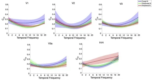
As we did with our psychophysical data, we looked at the mean zero point of thefirst derivatives of the bootstrapped polynomialfits to our C50 values tofind, for each ROI and eccentricity, the temporal frequency at which contrast sensitivity peaks. These zero points are presented in Ap-pendix Table B.2 and examples of bootstrappedfits are illustrated inFig. 9. In V1 and V2, the optimal temporal frequency gradually increased with eccentricity. However, in V3 and V3a the optimal temporal frequency increased from foveal to parafoveal. In hV4 the optimal temporal frequency is essentially identical between the foveal and parafovea. Fits to the data in the periphery of hV4 (see hV4 ofFig. 9) were almost linear and no peak could be computed reliably. We attribute this to variability within the hV4 C50estimates that were derived from the bootstrapping procedure. Thus, the

Fig. 7. Psychophysical contrast detection thresholds plotted as a function of temporal frequency, at two eccentricities. In A) we present contrast detection thresholds plotted at four measured temporal frequencies at 2_{and 10. In B) we present bootstrappedfits to contrast detection thresholds plotted as a function of temporal} frequency at 2_{and 10. Overall, there is little difference in sensitivity at each temporal frequency between fovea and near periphery.}

peripheral hV4fits presented here appear to differ when compared to the corresponding mean hV4 C50values as presented inFig. 10.

3.6. Peripherally tuned pRFs have increased contrast sensitivity at 20 Hz in V1, V2, V3, and V3a

A simple effects analysis was undertaken to explore differences in

contrast sensitivity within each ROI at each temporal frequency, comparing between foveal, parafoveal, and peripherally tuned pRFs. Sidak corrections were applied to all possible comparisons. Mean C50 values at all temporal frequencies and at 20 Hz alone are presented in

Fig. 10. We found eccentricity-dependent differences in contrast sensi-tivity at 20 Hz. Namely, we found that in V1, V2, V3, and V3a, C50at 20 Hz was consistently decreased in peripherally tuned pRFs when

Fig. 9. Examples of bootstrapped polynomialfits to C50values plotted as a function of temporal frequency for each eccentricity in all ROIs. The solid line is a second-order bootstrapped polynomialfit to the data and the shaded outline is the standard deviation of 2000 permutations.

compared to foveally tuned pRFs (p<_{.05), reflecting increased contrast}

sensitivity at a high temporal frequency in the cortical periphery. There was no difference in contrast sensitivity as a function of eccentricity at 1, 5, or 10 Hz, in any ROI. InFig. 11we present a surface-based average (N¼19) contrast sensitivity map at 20 Hz, projected onto an inflated cortical mesh. Similar to previous psychophysical sensitivities, contrast sensitivity in hV4 was invariant across eccentricity at all temporal fre-quencies tested, including 20 Hz. Allp-values are presented in Appendix Table A.7.

3.7. Comparing psychophysical and fMRI contrast sensitivities

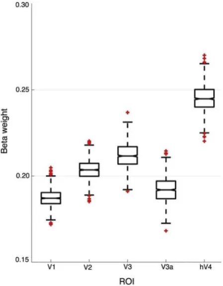
Unlike earlier visual areas, we found that contrast sensitivity at 20 Hz in hV4 was relatively invariant across eccentricity. Thisfinding is more similar to psychophysical sensitivities from our own and other behav-ioural studies that report little difference in temporal contrast sensitivity across visual space (Koenderink et al., 1978;Virsu et al., 1982;Wright and Johnston, 1983). Next, we aimed to examine the relationship be-tween psychophysical performance and fMRI signals driven by 20 Hz stimuli. Here, we bootstrapped 1000 estimates of 20 Hz fMRI C50 mea-surements from the fovea and periphery of each ROI, and fed this data into a linear model to assess how each ROI contributed to afit of psy-chophysical contrast sensitivity at 20 Hz. As illustrated inFig. 12, we found that C50values from hV4 contributed proportionally more to our psychophysical measurements when compared to early visual areas, indicating that fMRI responses from this area best predict our psycho-physical measurements. Bootstrapped beta weight statistics are available in Appendix Table B.3.

4. Discussion

We have measured differences in psychophysical and cortical contrast sensitivity that occur as a function of temporal frequency and visualfield eccentricity. Overall, ourfindings indicate that both psychophysical and cortical contrast sensitivity follow a‘U’shape function and is maximal between 8 and 12 Hz across visual space. Further, in early visual areas there is a relative increase in contrast sensitivity at 20 Hz in pRFs tuned to more peripheral regions of the visualfield. We discuss thesefindings in light of the physiological bias towards faster visual processing and

increased contrast sensitivity in the peripheral retina. As we progressed up the visual pathway to visual area hV4, we observed an equalisation of temporal contrast sensitivity across eccentricity that was closer to psy-chophysical measurements, suggesting that the peripheral bias in retinal temporal contrast sensitivity disappears in this cortical area.

Fig. 11.Mean contrast sensitivity maps at 20 Hz projected onto a cortical mesh (N¼19). Early visualfield maps V1–V3a show decreasing C50(indicating increasing contrast sensitivity) with increasing eccentricity, whilst contrast sensitivity in hV4 is invariant (and relatively low) across space.

and 10_{eccentricity, respectively. Similarly, in our fMRI data we found}

contrast sensitivity generally peaked around 8 Hz, with the critical fre-quency of this peak increasing between foveal and peripheral voxels. In this respect, the overall‘U’shape of our behavioural and cortical contrast sensitivity functions appears to be matched from a relatively early stage in the visual hierarchy.

Perhaps surprisingly, previous research has found little change in psychophysical temporal contrast sensitivity as a function of eccentricity (Koenderink et al., 1978;Rovamo and Raninen, 1984;Virsu et al., 1982). Although our own psychophysical data showed a slight decrease in temporal contrast sensitivity from the fovea to the near periphery, these differences were relatively small and may reflect difficulties in compensating precisely for cortical magnification effects or stimulus sizing in our own psychophysics (Granit and Harper, 1930;Hassan et al., 2016).

4.2. Peripherally tuned pRFs have increased contrast sensitivity at 20 Hz

Physiological biases in the response properties of retinal cells lead to increased temporal contrast sensitivity in more peripheral regions of the retina. Peripheral cones respond faster than foveal cones, resulting in greater peripheral sensitivity to rapidly changing input (Sinha et al., 2017). There is also an eccentricity-dependent increase in the ratio of parasol to midget RGCs, and parasol cells are relatively more sensitive to high temporal frequencies and have increased contrast gain when compared to midget cells (Connolly and van Essen, 1984;Dacey, 1993,

1994; Dacey and Petersen, 1992; De Monasterio and Gouras, 1975;

Schein and de Monasterio, 1987). At 10_{eccentricity, measurements}

of temporal contrast sensitivity are thought to reflect more isolated functions of parasol RGCs (Croner and Kaplan, 1995;Gouras, 1968;

Kaplan et al., 1990;Kaplan and Shapley, 1986). Signals passed from RGCs pass through the LGN, where the density of afferent parasol and midget RGCs is maintained, before being sent to primary visual cortex (Connolly and van Essen, 1984;Schein and de Monasterio, 1987). Our data show that a sensitivity bias similar to that found in the retina and LGN is present in early visual cortex, with relatively increased contrast sensitivity at 20 Hz in peripherally tuned voxels.

It is well known that neuronal spatial frequency sensitivity tends to be inversely related to temporal frequency sensitivity, thus, channels sen-sitive to low spatial frequencies are often sensen-sitive to higher temporal frequencies (and vice versa). In addition, the sensitivity of these channels changes as a function of eccentricity (D'Souza et al., 2016;Henriksson et al., 2008;Kulikowski and Tolhurst, 1973;Shoham et al., 1997;Sun et al., 2007). Here, we report measurements made at a single spatial frequency (1 cpd). This frequency was chosen because it is well below the spatial resolution limit at the highest eccentricities measured, yet gen-erates robust responses in the fovea (D'Souza et al., 2016;Henriksson et al., 2008;Welbourne et al., 2018). It is possible that our results would change if a different spatial frequency was used: altering the base spatial frequency might, for example, alter the balance of parvo-to magnocel-lular cells contributing to the stimulus at each eccentricity, which would, in turn, alter the average temporal response properties (Levitt et al., 2001).

low-level features, including contrast and temporal frequency, and instead represent more complex stimulus aspects relating to shape, identity, and colour (Avidan et al., 2002;Felleman and Van Essen, 1991;

Milner and Goodale, 1995;Perry and Fallah, 2014). For example, hV4 has previously been found to have a much coarser representation of spatial frequency and an increased tolerance to temporal dynamics when compared to earlier visual areas, suggesting these areas are less con-cerned with such low level visual properties (Henriksson et al., 2008;

Zhou et al., 2017). In a similar vein, ventral regions local to hV4 that are concerned with global form and object representations such as FFA, PPA, VO, and LOC, have at times found to be invariant to lower level visual features, and fMRI responses within such regions can become impaired when stimuli are presented at high temporal frequencies (D'Souza et al., 2011;Grill-Spector et al., 1999;Jiang et al., 2007;Kanwisher, 2010;Liu and Wandell, 2005;Mckeeff et al., 2007;Vernon et al., 2016). Although this bias in retinal temporal contrast sensitivity is phased out by hV4, our data found that this area also responds optimally around 10 Hz temporal frequency–perhaps inheriting this sensitivity bias from earlier regions.

5. Conclusion

Our experiments have found that in general, psychophysical and fMRI measurements of contrast sensitivity are relatively consistent and both peak around 8 Hz. Next, pRFs in early visual areas that represent more peripheral regions of visual space show relatively increased contrast sensitivity at a high temporal frequency when compared to those in the cortical representation of the fovea. However, this bias in peripheral cortical contrast sensitivity disappears by hV4, suggesting a relative in-dependence of temporal contrast sensitivity across space in this area. This independence is broadly consistent with behavioural measurements of temporal contrast sensitivity, and suggests that neurons in area hV4 (and possibly other higher-order ventral regions) are relatively invariant to the eccentricity-dependent biases that are present in the early visual stream.

Author contributions

M.M.H and A.R.W conceived and designed the experiments, M.M.H performed the experiments, M.M.H and A.R.W analysed the data, M.M.H wrote the paper, and M.M.H and A.R.W revised the paper.

Declaration of interest

The authors declare no competingfinancial interests.

Acknowledgements

Appendix C. Supplementary data

Supplementary data to this article can be found online athttps://doi.org/10.1016/j.neuroimage.2018.09.049.

Appendix A. Statistical output for pRF size normalisation statistics, ANOVA main effects, and simple effects analyses (*<.05, **<.01,

***<.001)

Table A.1

Normalized pRF sizes for each ROI (N¼19). For each ROI, small pRFs fall between the minimum and median pRF size, and large pRFs fall between median and maximum pRF size.

Visual Area Min pRF size Median pRF size Max pRF size

V1 0.25 _{1.72 9.89}

V2 0.25 _{2.06 9.30}

V3 0.25 _{2.89 9.74}

V3a 0.25 _{4.06 10.0}

hV4 0.25 _{4.7 10.0}

Table A.2

Tests of within-subjects effects for psychophysical data. Temporal frequency and eccentricity as IVs, and contrast detection threshold as DV.

Source df F pη2 p

Temporal Frequency (GG) 1.895 88.179 .830 .000***

Eccentricity 1 3.824 .175 .066

TF*Eccentricity (GG) 2.210 23.459 .566 .000***

Table A.3

Simple effects comparisons for psychophysical data. Differences in contrast detection thresholds, comparing between two factors of eccentricity at each temporal frequency (N¼19).

Temporal Frequency 10

1 Hz 2 _.000***

5 Hz 2 _.946

10 Hz 2 _.057

20 Hz 2 _.000***

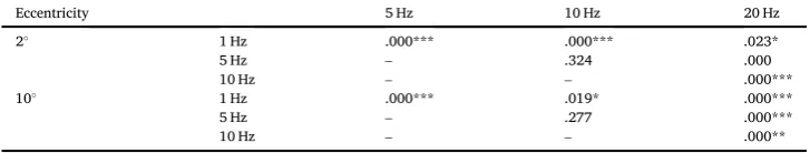
Table A.4

Simple effects comparisons for psychophysical data. Differences in contrast detection thresholds, comparing between four factors of temporal frequency at each eccentricity (N¼19).

Eccentricity 5 Hz 10 Hz 20 Hz

2 _{1 Hz .000*** .000*** .023*}

5 Hz – .324 .000

10 Hz – – .000***

10 _{1 Hz .000*** .019* .000***}

5 Hz – .277 .000***

10 Hz – – .000**

Table A.5

Tests of within-subjects effects for fMRI data. ROI, eccentricity, and temporal frequency as IVs, and C50as DV (N¼19).

Source df F p power

ROI (GG) 2.749 .684 .554 .177

Eccentricity 2 6.403 .004** .875

TF 3 4.466 .007** .853

ROI*Eccentricity (GG) 4.334 2.158 .077 .838

ROI*TF (GG) 5.977 1.638 .145 .602

Eccentricity*TF (GG) 2.911 2.132 .110 .504

V3a 1 Hz .813 .045* 1.000

5 Hz – .642 .919

10 Hz – – .037*

hV4 1 Hz .969 .124 .924

5 Hz – .595 .549

10 Hz – – .004**

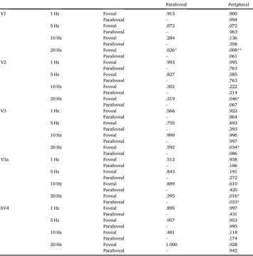
Table A.7

Simple effects for fMRI data. Differences in C50, comparing between three factors of eccentricity at each temporal

frequency within each ROI (N¼19).

Parafoveal Peripheral

V1 1 Hz Foveal .913 .900

Parafoveal – .994

5 Hz Foveal .072 .072

Parafoveal – .963

10 Hz Foveal .284 .136

Parafoveal – .358

20 Hz Foveal .026* .008**

Parafoveal – .061

V2 1 Hz Foveal .993 .995

Parafoveal – .763

5 Hz Foveal .827 .585

Parafoveal – .763

10 Hz Foveal .302 .222

Parafoveal – .214

20 Hz Foveal .319 .046*

Parafoveal – .067

V3 1 Hz Foveal .566 .922

Parafoveal – .864

5 Hz Foveal .755 .893

Parafoveal – .393

10 Hz Foveal .999 .996

Parafoveal – .997

20 Hz Foveal .592 .034*

Parafoveal – .086

V3a 1 Hz Foveal .512 .938

Parafoveal – .186

5 Hz Foveal .843 .191

Parafoveal – .272

10 Hz Foveal .889 .610

Parafoveal – .420

20 Hz Foveal .395 .016*

Parafoveal – .033*

hV4 1 Hz Foveal .895 .997

Parafoveal – .431

5 Hz Foveal .957 .953

Parafoveal – .995

10 Hz Foveal .481 .118

Parafoveal – .174

20 Hz Foveal 1.000 .928

Appendix B. Statistical output for bootstrapped psychophysics and fMRI data, and linear model results

Table B.1

Bootstrapped descriptive statistics psychophysical data (2000 iterations). Mean of the zero points of thefirst derivative of our bootstrappedfits to contrast threshold data, which is representative of the temporal frequency at which psy-chophysical contrast sensitivity peaks.

Bootstrap Distribution Mean Bootstrap Distribution Median SD

2 _{9.00 8.92 .58}

10 _{6.60 6.54 .57}

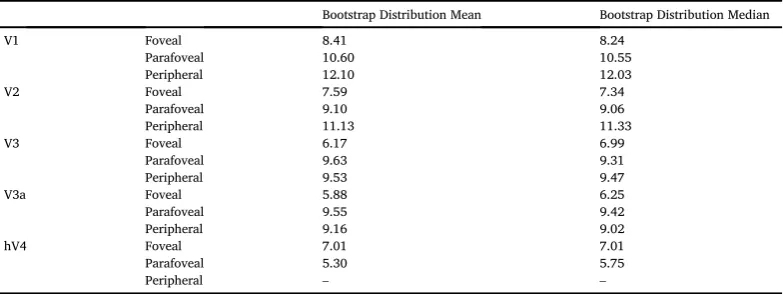
Table B.2

Bootstrapped descriptive statistics for fMRI data (2000 iterations). Mean of the zero points of thefirst derivative of our boot-strappedfits to C50data, which is representative of the temporal frequency at which fMRI contrast sensitivity peaks.

Bootstrap Distribution Mean Bootstrap Distribution Median

V1 Foveal 8.41 8.24

Parafoveal 10.60 10.55

Peripheral 12.10 12.03

V2 Foveal 7.59 7.34

Parafoveal 9.10 9.06

Peripheral 11.13 11.33

V3 Foveal 6.17 6.99

Parafoveal 9.63 9.31

Peripheral 9.53 9.47

V3a Foveal 5.88 6.25

Parafoveal 9.55 9.42

Peripheral 9.16 9.02

hV4 Foveal 7.01 7.01

Parafoveal 5.30 5.75

Peripheral – –

Table B.3

Bootstrapped beta weight estimates (1000 iterations) after feeding foveal and peripheral 20Hz C50values

into a linear model to assess how each ROI contributed to afit of psychophysical contrast sensitivity.

ROI Bootstrap Median Beta Weight

V1 0.18

V2 0.21

V3 0.22

V3a 0.19

hV4 0.24

References

Albrecht, D.G., Hamilton, D.B., 1982. Striate cortex of monkey and cat: contrast response function. J. Neurophysiol. 48 (1), 217–237. https://doi.org/0022-3077/82/0000-0000$01.25.

Avidan, G., Harel, M., Hendler, T., Ben-bashat, D., Zohary, E., Papanikolaou, A., Smirnakis, S.M., 2002. Contrast sensitivity in human visual areas and its relationship to object recognition. J. Neurophysiol. 87 (6), 3102–3116.https://doi.org/10.1152/ jn.2002.87.6.3102.

Boynton, G.M., Demb, J.B., Glover, G.H., Heeger, D.J., 1999. Neuronal basis of contrast discrimination. Vis. Res. 39 (2), 257–269.https://doi.org/10.1016/S0042-6989(98) 00113-8.

Brainard, D.H., 1997. The psychophysics toolbox. Spatial Vis. 10 (4), 433–436.https:// doi.org/10.1163/156856897X00357.

Connolly, M., van Essen, D., 1984. The representation of the visualfield in parvocellular and magnocellular layers in the lateral geniculate nucleus in the macque monkey. J. Comp. Neurol. 226 (4), 544–564.https://doi.org/10.1002/cne.902260408. Croner, L.J., Kaplan, E., 1995. Receptivefields of P and M ganglion cells across the

primate retina. Vis. Res. 35 (1), 7–24.https://doi.org/10.1016/0042-6989(94) E0066-T.

D'Souza, D., Auer, T., Frahm, J., Strasburger, H., Lee, B.B., 2016. Dependence of chromatic responses in V1 on visualfield eccentricity and spatial frequency: an fMRI study. J. Opt. Soc. Am. A 33 (3), 53–64.https://doi.org/10.1364/JOSAA.33.000A53. D'Souza, D., Auer, T., Strasburger, H., Frahm, J., Lee, B.B., 2011. Temporal frequency and chromatic processing in humans : an fMRI study of the cortical visual areas. J. Vis. 11, 1–17, 2011.https://doi.org/10.1167/11.8.8.

Dacey, D.M., 1993. The mosaic of midget ganglion cells in the human retina. J. Neurosci. 13 (12), 5334–5355.https://doi.org/10.1523/JNEUROSCI.13-12-05334.1993.

Dacey, D.M., 1994. Physiology, morphology and spatial densities of identified ganglion cell types in primate retina. In: Higher-order Processing in the Visual System. Ciba Foundation, London, pp. 12–34.

Dacey, D.M., Petersen, M.R., 1992. Dendriticfield size and morphology of midget and parasol ganglion cells of the human retina. Proc. Natl. Acad. Sci. U.S.A. 89 (20), 9666–9670.https://doi.org/10.1073/pnas.89.20.9666.

De Monasterio, F.M., Gouras, P., 1975. Functional properties of ganglion cells of the rhesus monkey retina. J. Physiol. 25 (1), 167–195.https://doi.org/10.1113/jphysiol. 1975.sp011086.

Drasdo, N., Fowler, C.W., 1974. Non-linear projection of the retinal image in a wide-angle schematic eye. Br. J. Ophthalmol. 58 (8), 709–714.https://doi.org/10.1136/bjo.58. 8.709.

Dumoulin, S.O., Wandell, B.A., 2008. Population receptivefield estimates in human visual cortex. Neuroimage 39 (2), 647–660.https://doi.org/10.1016/j.neuroimage. 2007.09.034.

Engel, S.A., Glover, G.G., Wandell, B.A., 1997. Retintopic organization in human visual cortex and the spatial precision of functional MRI. Cerebr. Cortex 7 (2), 181–192. https://doi.org/10.1093/cercor/7.2.181.

Enroth-Cugell, C., Shapley, R.M., 1973. Adaptation and dynamics of cat retinal ganglion cells. J. Physiol. 233 (2), 271–309.https://doi.org/10.1113/jphysiol.1973. sp010308.

Felleman, D.J., Van Essen, D.C., 1991. Distributed hierachical processing in the primate cerebral cortex. Cerebr. Cortex 1 (1), 1–47.https://doi.org/10.1093/cercor/1.1.1. Friston, K.J., Fletcher, P., Josephs, O., Holmes, A., Rugg, M.D., Turner, R., 1998.

Event-related fMRI: characterizing differential responses. Neuroimage 7 (1), 30–40.https:// doi.org/10.1006/nimg.1997.0306.

Hawken, M.J., Shapley, R.M., Grosof, D.H., 1996. Temporal-frequency selectivity in monkey visual cortex. Vis. Neurosci. 13, 477–492, 1996.https://doi.org/10.1017/ S0952523800008154.

Henriksson, L., Nurminen, L., Hyvarinen, A., Vanni, S., 2008. Spatial frequency tuning in human retinotopic visual areas. J. Vis. 8 (10), 1–13.https://doi.org/10.1167/8.10.5. Horiguchi, H., Nakadomari, S., Masaya, M., Wandell, B.A., 2009. Two temporal channels in human V1 identified using fMRI. Neuroimage 47 (1), 273–280.https://doi.org/10. 1016/j.neuroimage.2009.03.078.

Jenkinson, M., Beckmann, C.F., Behrens, T.E.J., Woolrich, M.W., Smith, S.M., 2012. Fsl. NeuroImage62 (2), 782–790.https://doi.org/10.1016/j.neuroimage.2011.09.015. Jiang, Y., Zhou, K., He, S., 2007. Human visual cortex responds to invisible chromatic

flicker. Nat. Neurosci. 10 (5), 657–662.https://doi.org/10.1038/nn1879. Kanwisher, N., 2010. Functional specificity in the human brain: a window into the

functional architecture of the mind. Proc. Natl. Acad. Sci. Unit. States Am. 107 (25), 11163–11170.https://doi.org/10.1073/pnas.1005062107.

Kaplan, E., Lee, B.L., Shapley, R.M., 1990. New views of primate retinal functions. In: Osborne, N., Chader, G.J. (Eds.), Progress in Retinal Research. Pergamon Press, Elmsford, NY, pp. 273–335.

Kaplan, E., Shapley, R., 1986. The primate retina contains two types of ganglion cells, with high and low contrast sensitivity. Proc. Natl. Acad. Sci. U.S.A. 83 (8), 2755–2757.https://doi.org/https://doi.org/10.1073/pnas.83.8.2755. Kastner, S., O'Connor, D.H., Fukui, M.M., Fehd, H.M., Herwig, U., Pinsk, M.A., 2004.

Functional imaging of the human lateral geniculate nucleus and pulvinar. J. Neurophysiol. 91 (1), 438–448.https://doi.org/10.1152/jn.00553.2003. Koenderink, J.J., Bouman, M.A., Bueno, A.E., Slappendel, S., 1978. Perimetry of contrast

detection thresholds of moving spatial sine wave patterns. I. The near peripheral visualfield (eccentricity 0_{–8). J. Opt. Soc. Am. 68 (6), 845–849.https://doi.org/} 10.1364/JOSA.68.000845.

Kontsevich, L.L., Tyler, C.W., 1999. Bayesian adaptive estimation of psychometric slope and threshold. Vis. Res. 39 (16), 2729–2737. https://doi.org/10.1016/S0042-6989(98)00285-5.

Kulikowski, J.J., Tolhurst, D.J., 1973. Psychophysical evidence for sustained and transient detectors in human vision. J. Physiol. 232 (1), 149–162.https://doi.org/10. 1113/jphysiol.1973.sp010261.

Kwong, K.K., Belliveau, J.W., Chesler, D.A., Goldberg, I.E., Weisskoff, R.M., Poncelet, B.P., Turner, R., 1992. Dynamic magnetic resonance imaging of human brain activity during primary sensory stimulation. Proc. Natl. Acad. Sci. U.S.A. 89 (12), 5675–5679. https://doi.org/10.1073/pnas.89.12.5675.

Levitt, J.B., Schumer, R.A., Sherman, S.M., Spear, P.D., Movshon, J.A., 2001. Visual response properties of neurons in the LGN of normally reared and visually deprived macaque monkeys. J. Neurophysiol. 85 (5), 2111–2129. Retrieved from.http:// www.ncbi.nlm.nih.gov/pubmed/11353027.

Liu, J., Wandell, B.A., 2005. Specializations for chromatic and temporal signals in human visual cortex. J. Neurosci. 25 (13), 3459–3468.https://doi.org/10.1523/ JNEUROSCI.4206-04.2005.

Mckeeff, T.J., Remus, D.A., Tong, F., 2007. Temporal limitations in object processing across the human ventral visual pathway. J. Neurophysiol. 98 (1), 382–393.https:// doi.org/10.1152/jn.00568.2006.

and retinal illuminance. Vis. Res. 24 (10), 1127–1131.https://doi.org/10.1016/ 0042-6989(84)90166-4.

Rovamo, J., Virsu, V., 1979. An estimation and application of the human cortical magnification factor. Exp. Brain Res. 37 (3), 495–510.https://doi.org/10.1007/ BF00236819.

Schein, S.J., de Monasterio, F.M., 1987. Mapping of retinal and geniculate neurons onto striate cortex of macaque. J. Neurosci. 7 (4), 996–1009.https://doi.org/10.1523/ JNEUROSCI.07-04-00996.1987.

Shoham, D., Hübener, M., Schulze, S., Grinvald, A., Bonhoeffer, T., 1997. Spatio-temporal frequency domains and their relation to cytochrome oxidase staining in cat visual cortex. Nature 385, 529–533.https://doi.org/10.1038/385529a0.

Singh, K.D., Smith, A.T., Greenlee, M.W., 2000. Spatiotemporal frequency and direction sensitivities of human visual areas measured using fMRI. Neuroimage 12 (5), 550–564.https://doi.org/10.1006/nimg.2000.0642.

Sinha, R., Hoon, M., Baudin, J., Okawa, H., Wong, R.O.L., Rieke, F., 2017. Cellular and circuit mechanisms shaping the perceptual properties of the primate fovea. Cell 168 (3), 413–426 e12.https://doi.org/10.1016/j.cell.2017.01.005.

Sun, P., Ueno, K., Waggoner, R.A., Gardner, J.L., Tanaka, K., Cheng, K., 2007. A temporal frequency-dependent functional architecture in human V1 revealed by high-resolution fMRI. Nat. Neurosci. 10 (11), 1404–1406.https://doi.org/10.1038/ nn1983.

Teo, P.C., Sapiro, G., Wandell, B.A., 1997. Creating connected representations of cortical gray matter for functional MRI visualization. IEEE Trans. Med. Imag. 16 (6), 852–863.https://doi.org/10.1109/42.650881.

Venkataraman, A.P., Lewis, P., Unsbo, P., Lundstr€om, L., 2017. Peripheral resolution and contrast sensitivity: effects of stimulus drift. Vis. Res. 133, 145–149.https://doi.org/ 10.1016/j.visres.2017.02.002.

Vernon, R.J.W., Gouws, A.D., Lawrence, S.J.D., Wade, A.R., Morland, A.B., 2016. Multivariate patterns in the human object-processing pathway reveal a shift from retinotopic to shape curvature representations in lateral occipital areas, 1 and LO-2. J. Neurosci. 36 (21), 5763–5774.https://doi.org/10.1523/JNEUROSCI.3603-15. 2016.

Virsu, V., Rovamo, J., Laurinen, P., N€as€anen, R., 1982. Temporal contrast sensitivity magnification and cortical magnification. Nature 22 (9), 1211–1217.https://doi.org/ 10.1016/0042-6989(82)90087-6.

Wandell, B.A., Dumoulin, S.O., Brewer, A.A., 2007. Visualfield maps in human cortex. Neuron 56 (2), 366–383.https://doi.org/10.1016/j.neuron.2007.10.012. Welbourne, L.E., Morland, A.B., Wade, A.R., 2018. Population receptivefield (pRF)

measurements of chromatic responses in human visual cortex using fMRI. Neuroimage 167, 84–94. May 2017.https://doi.org/10.1016/j.neuroimage.2017.11. 022.

Wright, M.J., Johnston, A., 1983. Spatiotemporal contrast sensitivity and visualfield locus. Vis. Res. 23 (10), 983–989.https://doi.org/10.1016/0042-6989(83)90008-1. Zhou, J., Benson, N.C., Kay, K., Winawer, J., 2017. Compressive temporal summation in