RESEARCH PAPER
Constitutive modelling of granular materials using a contact
normal-based fabric tensor
Nian Hu1,3•Hai-Sui Yu2•Dun-Shun Yang4•Pei-Zhi Zhuang2,3
Received: 8 August 2018 / Accepted: 8 April 2019 The Author(s) 2019
Abstract
This paper presents a fabric tensor-based bounding surface model accounting for anisotropic behaviour (e.g. the depen-dency of peak strength on loading direction and non-coaxial deformation) of granular materials. This model is developed based on a well-calibrated isotropic bounding surface model. The yield surface is modified by incorporating the back stress which is proportional to a contact normal-based fabric tensor for characterising fabric anisotropy. The evolution law of the fabric tensor, which is dependent on both rates of the stress ratio and the plastic strain, rules that the material fabric tends to align with the loading direction and evolves towards a unique critical state fabric tensor under monotonic shearing. The incorporation of the evolution law leads to a rotational hardening of the yield surface. The anisotropic critical state is assumed to be independent of the initial values of void ratio and fabric tensor. The critical state fabric tensor has the same intermediate stress ratio (i.e.bvalue) and principal directions as the critical state stress tensor. A non-associated flow rule in the deviatoric plane is adopted, which is able to predict the non-coaxial flow naturally. The stress–strain relation and fabric evolution of model predictions show a satisfactory agreement with DEM simulation results under monotonic shearing with different loading directions. The model is also validated by comparing with laboratory test results of Leighton Buzzard sand and Toyoura sand under various loading paths. The comparison results demonstrate encouraging applicability of the model for predicting the anisotropic behaviour of granular materials.
Keywords Anisotropic critical state Fabric anisotropyFabric evolution lawLoading direction Non-coaxial flow Rotational hardening
1 Introduction
Fabric anisotropy has a significant influence on the strength and deformation characteristics of granular materials as reported in both experimental [3,41,46–48,50,77,84,88] and numerical observations [34, 69, 81, 86]. In the past
years, various effects caused by fabric anisotropy have been taken into account in constitutive models using dif-ferent concepts.
The concept of rotational hardening, first proposed by Sekiguchi [64], has been widely used in constitutive modelling of geomaterials for describing initial anisotropy
& Pei-Zhi Zhuang [email protected] Nian Hu
[email protected] Hai-Sui Yu [email protected] Dun-Shun Yang [email protected]
1 Nottingham Centre for Geomechanics, Faculty of
Engineering, The University of Nottingham, University Park, Nottingham NG7 2RD, UK
2 School of Civil Engineering, University of Leeds, Leeds LS2 9JT, UK
3 State Key Laboratory for GeoMechanics and Deep Underground Engineering, China University of Mining and Technology No, 1 Daxue Road, Xuzhou, Jiangsu 221116, China
as well as induced anisotropy (e.g. [2, 10, 20, 27, 54, 67, 76]). Hashiguchi [19] discussed similarities and differences between the rotational hard-ening and the kinematic hardhard-ening [98] for metals. There are several general features of the rotational hardening rule in general stress spaces:
• A second-order traceless anisotropy tensor is used to reflect the material anisotropy, and it is introduced into the yield function through the back stress concept;
• The evolution of the anisotropy tensor is linked to the plastic strain rate. The tensor can reach a ‘saturated’ value [2] under monotonic shearing. In other words, the anisotropy tensor stops changing at large strains, for example, by introducing a rotational limit surface [20].
In the concept of rotational hardening, the anisotropy tensor, in general, is indirectly linked to the material fabric based on some microscopic evidence, but usually lacks clear physical meaning at a microscopic level. Hence the evolution of the tensor is hard to be calibrated directly even while microstructural information is available.
Recently, several constitutive models have been pro-posed using different fabric tensors associated with various microstructural quantities (see the references of [33, 73]) such as the orientation of the long axis of particles [30,31], void vector [14, 32] and contact normal [1, 96, 97]. As contacts may represent the most fundamental fabric of granular materials, contact normal-based fabric tensors receive increasing attention, and potential effects of the fabric anisotropy show a strong link to this fabric tensor. Micromechanical analyses of the stress–force–fabric rela-tionship showed that anisotropy of the orientation distri-bution of contact normals (or anisotropy of the contact normal-based fabric tensor) may play an important role in contributing to the shear strength of granular materials [35,52,60]. Meanwhile, the non-coincidence between the fabric tensor and the stress tensor is a key source of non-coaxial deformation [36].
In evolution laws of contact normal-based fabric tensors, the rate of the fabric tensor has often been related to stress rate [75], elastic strain rate [96, 97], or plastic strain rate [42,43]. As the elastic strain rate and stress rate can be easily linked by an elastic model, the responses of evolu-tion laws in terms of them are essentially similar. Evoluevolu-tion laws associated with the stress (or elastic strain) rate alone (the first type) can capture the characteristics of peak strength under monotonic shearing with various loading directions. However, they rarely show a unique critical state fabric tensor. On the contrary, fabric evolution laws associated with the plastic strain rate alone (the second type) tend to give a unique critical value of the fabric tensor, but they cannot capture the characteristics of peak strength upon monotonic shearing easily. Although these
types of evolution laws may be able to qualitatively account for some experimental and numerical observations, quantitative calibrations with microscale fabric evolution data have rarely been achieved.
Most of the above-mentioned constitutive models, incorporating either a rotational hardening or a fabric tensor, are based on the critical state concept which has been widely recognised as the cornerstone of modern constitutive modelling of soils [63, 78]. Conventionally, the critical state is defined as a state at which the soil behaves like a frictional fluid with a constant void ratio and stress ratio, regardless of the initial state of the soil. It is clear that this definition makes no reference to other fabric-related entities than the scalar-valued void ratio. Consequently, it cannot provide necessary constraints on the evolution of the anisotropic fabric towards the critical state. However, microstructural investigations reveal that material fabric at the critical state is anisotropic [61] and contact normal-based fabric tensors at the critical state seem to be independent of the initial fabric [22, 81, 82, 95]. For more realistically modelling the anisotropic behaviour within the framework of the critical state concept, it is necessary to revisit the conventional critical state theory [9,32].
The main aim of this paper is to present a critical state constitutive model for granular materials taking the fabric anisotropy into account. The model is developed on the basis of the isotropic bounding surface model named CASM_b [89,90]. A contact normal-based fabric tensor is additionally incorporated, and its evolution is formulated by using the hybrid evolution law proposed by the first author [21]. In the new hybrid evolution law, the rate of the fabric tensor is related to both the stress ratio rate and the deviatoric plastic strain rate.
In short, the model can capture the following common effects of fabric anisotropy on the strength and deformation behaviour of granular materials:
• the dependency of the peak strength on loading directions;
• the uniqueness of the anisotropic critical state under different loading directions with a constantbvalue and mean effective stress;
• the non-coaxial plastic flow.
2 Anisotropic critical state
2.1 Definition of fabric tensor
In most cases of three-dimensional materials, the frequency distribution of contact normals in a granular assembly can be expressed by a spherical harmonic series with the sec-ond-order approximation [21,93] as
Eð Þ ¼n 1
4pð1þF:nnÞ ð1Þ
where n denotes the unit contact normal at a contact. According to Kanatani [23], the tensor F in Eq. (1) is known as the second-order fabric tensor of the third kind in terms of unit contact normals. The fabric tensor F is traceless, and it can be used to describe fabric anisotropy in the assembly. Practically, the fabric tensorF can be esti-mated as follows:
F¼15 2
1 Nc
X
c2Nc
ncnc1 3I
!
ð2Þ
whereIdenotes unit second-order tensor andNcis the total number of discrete directional contact normal nc of a granular assembly.
2.2 Description of the anisotropic critical state
Since granular materials like sands usually lack a unique, natural stress-free state, the critical state is important for constitutive modelling as it provides a useful reference state to characterise the granular materials under shearing. Based on the critical state concept, many constitutive models have been proposed, including a series of CASMs by Yu [90]. However, the fabric anisotropy at the critical state is often overlooked. Benefiting from the development of advanced laboratory test [12, 83] and numerical simu-lation technologies [13,26,44,79,81,82,95], the fabric effect on the critical state is further studied in recent years (e.g. [30, 32, 85], in particular, from a microscopic per-spective. Increasing evidence shows that a unique critical state exists, which is independent of the initial sand density and the initial fabric anisotropy. In the light of the above discussion, the conventional definition of the critical state is revisited and modified considering the role of anisotropic fabric as follows.
The mean effective stress, p, and deviatoric stress ten-sor,S, can be expressed as:
p¼1=3trð Þr ð3Þ
S¼rpI ð4Þ
where r is the effective stress tensor. The intermediate stress ratio (i.e.bvalue) is given as:
b¼r2r3
r1r3
¼1 2
ffiffiffi 3 p
tanð Þ þhl 1
h i
ð5Þ
wherer1;r2;r3are the principal values ofrin descending order (i.e.r1[r2[r3), andhlis the Lode’s angle, which equals:
sin 3hlð Þ ¼ 3pffiffiffi6detð ÞS S
k k3 ð6Þ
wherek k ¼ pffiffiffiffiffiffiffiffiffi: denotes the norm of any symmetrical second-order tensor *. A stress ratio tensor can be defined as:
g¼S=p ð7Þ
The deviators of tensorsS;g;Fare rewritten as q;g;F, respectively.
q¼k3=2Sk ð8Þ
g¼k3=2gk ð9Þ
F¼k3=2Fk ð10Þ
The conventional definition of the critical state can be expressed in Eqs. (11) and (12), which describes that plastic shearing could continue indefinitely without chan-ges in volume or stress ratios while the critical state is ultimately reached. For characterising the anisotropic crit-ical state, an extra constraint on the fabric tensor at the critical state is defined in Eq. (13) [21].
ec¼ klnð Þ þpc C1; ð11Þ
gc¼M; ð12Þ
Fc¼ ðMF=MÞgc ð13Þ
where k and C are the slope and intercept of the critical state line in the vlnp space, respectively; M, so-called critical state stress ratio, is the slope of the critical state line in thep–qspace;gc;gcandFcare the values ofg,gandF at the critical state, receptively; MF is the critical state fabric ratio. Obviously, there is MF¼Fc whereFc is the value ofFat the critical state.
It should be noted that the critical state line in thee lnp plane might be nonlinear due to the breakage of par-ticles under relatively high pressure (normally greater than 1 MPa for silica sands) [5]. In this situation, the relation-ship between ec and lnpc is better to be replaced by a bilinear relationship [5] or a nonlinear relationship [28]. As the effect of particle breakage is ignored in this work, we adopt the same linear relationship betweenecand lnpc as that employed in the original CASM [89]. This relationship is valid until particle breakage occurs according to the results of laboratory tests [74,91], as shown in Fig.1. In a general stress space, it is found that both M and MF are dependent on thebvalue [93]. For simplicity, we first take MandMFas constants here, and their dependency on the bvalue will be discussed in Sect.3.6.
It should be noted that Li and Dafalias [32] proposed an alternative description of fabric anisotropy at the critical state by using a void-vector fabric tensor. They also argued that the critical state fabric tensor has the same principal directions and b value as those of the deviatoric stress tensor. A joint invariant consisting of the critical state fabric tensor normalised by kFck was adopted, and, as a
consequence,MFalways equals ffiffiffiffiffiffiffiffi 3=2 p
therein. As the back stress is more closely dependent on the fabric deviatorFc rather than the normalised value, the more direct analytical description of the critical state fabric tensor with respect to Fcdefined in Eq. (13) is used here while incorporating the fabric tensor into the yield function using the back stress concept as shown later.
2.3 Fabric evolution law
The rate of fabric tensorF_ is related to both the stress ratio rateg_ and the plastic strain rate in terms ofK_ ¼e_p where
_
ep is the deviatoric plastic strain rate. The hybrid fabric evolution law proposed by the first author [21] [i.e.
Eq. (14)] is used. The derivation and validation of the fabric evolution law refer to the reference of [21], and an extension for incorporating the intermediate stress ratio effect is presented in the Ref. [93].
_
F¼C1ð1þC2k kg Þg_þC3 MF
M gF
_
K ð14Þ
whereC1,C2andC3are material constants controlling the rate of the fabric evolution. At the critical stateF_ ¼0 and
_
g¼0, there should beFc¼MFgc=M. The evolution law satisfies the requirement of the principle of material frame indifference together with the assumptions of rate inde-pendence and uniqueness of the critical state fabric tensor [i.e. Eq. (13)] [21].
Initially, the plastic strain rate is small whereas the stress ratio increases rapidly under monotonic shearing. In this case, the fabric evaluation is dominated by variations of the stress ratio. The fabric evolution law (14), therefore, can be simplified as:
_
F¼C1ð1þC2k kg Þg_ ð15Þ
From Eq. (15), it can be deduced that the deviatorFqof the fabric tensor is formulated as a parabolic function of the stress ratiog under monotonic shearing. This is supported by experimental [49,75] and numerical results [25].
As shearing continues, the plastic strain rate increases considerably while the rate of the stress ratio drops, espe-cially, near the critical state. In this stage, the contribution of the second term of the right side of Eq. (14) prevails, and the fabric tensor evolves towards the critical state value of Eq. (13). In this case, the fabric evolution can be approximated by:
_
F¼C3 MF
M gF
_
K ð16Þ
Equations (15) and (16) are special cases of the hybrid evolution law of Eq. (14) while takingC3= 0 andC1= 0, respectively. It is clear that the parameters C1 and C2 control the rate of fabric evolution at the initial stage of a monotonic shearing, while C3 controls the rate of fabric evolution towards the critical state at relatively large strains. Upon continuous shearing, the evolution law tran-sitions from the first type to the second type gradually, and hence, the aforementioned disadvantages that exist in evolution laws taking the form of only one of them may be overcome.
From a microstructural perspective, the evolution laws (15) and (16) may roughly represent two typical mecha-nisms of fabric evolution, respectively [21, 93]. At the initial stage of shearing, contacts are forced to reorganise to stabilise the potential buckling of force chain responding to the applied shear stress [71]. At this stage, the stress ratio increases rapidly whereas plastic strains develop relatively
Mean effecve stress, p (kPa)
Sp
ec
ifi
c v
o
lu
m
e,
v=
1+e
Toyoura sand Portaway sand
0.025ln 1.800
v= − p+
0.031ln 2.0671
v= − p+
1.6 1.65 1.7 1.75 1.8 1.85 1.9 1.95
101 102 103 104
Fig. 1 Critical state lines in thevlnpplane for Toyoura sand and
[image:4.595.86.260.533.686.2]slowly. Therefore, changes in the spatial distribution of contact normals, i.e. evolution of the fabric tensor (e.g. a considerable amount of contact disruptions in the minor principal fabric direction and contact creations along the major principal fabric direction [25, 69]), are more effi-ciently expressed in terms of the rate of the stress ratio. At relatively large shear strains, the net rate of contact cre-ation/disruption decreases considerably. Instead, the fabric evolution is primarily controlled by the reorientation and migration of the contacts through sliding and rolling of particles across each other which is usually accompanied by more plastic deformation [25,26]. Therefore, the fabric evolution is more reasonably related to the plastic strain rate at this stage.
3 Constitutive model
This constitutive model is developed based on CASM_b [90] which is known as an isotropic critical state model using the bounding surface framework. A contact normal-based fabric tensor is incorporated into the yield surface and the flow rule in thep plane to account for fabric ani-sotropy, and the anisotropic critical state defined in Eq. (13) is adopted. However, it should be noted that no attempt is made to account for the potential effects of fabric anisotropy in the dilatancy function and the elastic model in this paper.
The constitutive model is presented in the general stress space. The model described here is applicable to both fully saturated and dry soils. All stress quantities are to be understood as effective stress quantities in this paper. Our attention is restricted to the small deformation regime, isothermal conditions and rate-independent behaviour. Thus, the strain rates are split as follows:
_
e¼e_eþe_p; _ev¼e_e vþe_
p
v ð17Þ
where e_;e_e;e_p are the rates of total, elastic and plastic deviatoric strains, respectively; ev_;e_e
v;e_ p
v are the rates of total, elastic and plastic volumetric strains, respectively.
3.1 Elastic model
The hypoelastic model used in CASM is followed here. Potential effects of the fabric anisotropy on the elastic behaviour are ignored as purely elastic strains are relatively small compared with plastic strains. The response associ-ated with the elastic volumetric part is expressed in terms of the bulk modulus K which is assumed to be a linear function of the mean effective stressp:
_
ee
v¼
_
p
K; K¼ð1þeÞp=j ð18Þ
where j is the slope of the swelling line in the vlnp plane.
The deviatoric elastic strain is calculated by using the shear modulus as:
_
ee¼ S_ 2G; G¼
3 1ð 2tÞ
2 1ð þtÞK ð19Þ
where tis Poisson’s ratio. A constant value of Poisson’s ratio is assumed, which implies that the shear modulus is dependent on the mean effective stress in the same way as the bulk modulus. The advantages and disadvantages of a constant Poisson’s ratio compared with a constant shear modulus were discussed by Yu [89]. Note that various other relationships of the shear modulus for uncemented sands at small strains have also been proposed in the lit-erature (e.g. [17]).
From Eqs. (18) and (19), the rate of the stress tensor can be expressed in terms of the strain rates as:
_
r¼2Ge_e_PþK ev_ e_Pv
I ð20Þ
3.2 Yield surface
Plastic deformation of granular materials with hard grains is induced in the process of sliding and rolling of indi-vidual grains across each other at contact points. As frictional resistance increases, rolling becomes more dominant. At a mesoscale, it may be assumed that dilatant simple shearing over several interacting sliding planes produces the resultant macroscopic deformation, which is often accompanied by induced fabric anisotropy. By applying the Mohr–Coulomb yield condition at sliding planes, Nemat-Nasser [42] proposed a yield surface con-sidering the fabric effect. The kernel idea is that the shear resistance at the sliding plane can be divided into two parts: an isotropic part due to a Coulomb-type isotropic resistance and an anisotropic part due to fabric anisotropy. The resistance due to fabric anisotropy is estimated by the micromechanically based stress–force–fabric relationship. From this approach, it was found that the back stress is proportional to the contact normal-based fabric tensor in a two-dimensional (2D) analysis. Actually, in this estima-tion it was assumed that the total back stress stems from an anisotropic stress tensor rr which is resulted from the fabric tensorF. Similarly, one can obtain the back stress Sb in the three-dimensional (3D) domain from the stress– force–fabric relationship obtained by Ouadfel and Rothenburg [52] as follows:
Sb ¼rr¼fpF; f¼2=5 ð21Þ
coefficient obtained by spatial integration of the stress– force–fabric relation. In a 2D case, the coefficientfequals 1/2 [60] as the same as that obtained by Nemat-Nasser [42]. The yield surface can be expressed in terms of stress tensor and fabric tensorFas:
f ¼kSfpFk Mfp¼0 ð22Þ
where Mf is the frictional coefficient, which is generally dependent on the void ratio and fabric tensor.Mfgives the elastic range of the yield surface. Back stress fpF deter-mines the location and orientation of the yield surface. If we regard that the isotropic yield surface used in CASM is a special case of Eq. (22), a suitable form ofMfin Eq. (22) can be chosen. The yield surface with the inclusion of the back stress can now be expressed as follows:
f ¼ q~ mp
n
þ 1
lnð Þr0 ln p p0
¼0 ð23Þ
~
q¼k3=2ðSSbÞk ð24Þ
where n and r0 are material constants; m¼M;p0 is the reference consolidation pressure. The conventional stress deviatorq¼k3=2Skis replaced byq. It is clear that when~
the material fabric is isotropic, namelySb¼0 in Eq. (24), Eq. (23) recovers the original yield function of CASM.
In the original CASM [89], the spacing ratio r was introduced to represent the distance between the reference consolidation line and the critical state line in thevlnp space. The spacing ratio can be calculated as r¼p0=pc wherepcis the mean effective stress at the critical state on a given yield surface. It is noted that this distance should remain unaltered for the anisotropic critical state model. With this assumption, the spacing ratioris replaced by a new material constantr0 using the following equation:
lnr0¼lnrð1fMF=MÞn ð25Þ
This equation is obtained by applying the critical state stress condition and fabric tensor [i.e. Eqs. (12) and (13)] to the yield function with the condition that p0=pc¼r. Through Eqs. (23) (24) and (25), the fabric tensor is introduced into the isotropic yield surface with clear physical meaning.
3.3 Hardening law
It is noted that the yield surface in Eq. (23), in fact, involves both isotropic and rotational hardening. At first, the isotropic hardening rule adopted in the original CASM [89] is followed. The size of the yield surface is controlled by the reference consolidation pressure p0 which varies with the plastic volumetric strain as defined in Eq. (26).
_
p0¼ð1þeÞp0
kj e_
p
v ð26Þ
If elastic strains are ignored, we can integrate Eq. (26) and then find thatp0can be expressed in terms of the void ratio. It indicates that the yield surface is dependent on the void ratio if p0 is replaced, which is consistent with the suggestion onMfby Nemat-Nasser and Zhang [43].
The rotational hardening is introduced due to the evo-lution law of the fabric tensor [i.e. Eq. (14)] as illustrated in Fig.2 in the triaxial stress space with a cross-anisotropy. The slope of the axis of the yield surface (i.e. green line) represents the degree of fabric anisotropy. Specifically, the slope is equal to 2/5(F1-F2) in the axial-symmetrical case. Upon shearing, the degree of fabric anisotropy varies as defined by the fabric evolution law (14). Therefore, the slope of the green line changes, which results in rotations of the yield surface in thep0-normalisedp–qspace. When the critical state is reached, the slope of the axis of the yield surface will rest on a value corresponding to the critical state value of the fabric anisotropy. Mathematically, Eq. (13) acts as a rotational limit surface of the anisotropy tensor [20]. It defines that rotational hardening of the yield surface will cease once the critical state is reached. One important feature of this law is that the fabric deviator F can both harden and soften as the stress ratio g might harden and soften during a monotonic shearing. The slope of the axis can be even larger than the critical state value as demonstrated by Hu [21].
3.4 Flow rule
From the viewpoint of thermodynamics [6, 7] and micromechanics [11], the flow rule is non-associated in
Normalised shear stress
, q/p
0
Normalised mean stress, p/p0
F1=0,F2=0,F3=0
F1=0.5,
F2=-0.25,F3=-0.25
F1=1,
F2=-0.5,F3=-0.5
Critical State Line: Compression
Critical State Line: Extension
Rotational Hardening
A
B C
-0.4 -0.2 0 0.2 0.4 0.6 0.8
0 0.1 0.2 0.3 0.4 0.5 0.6 0.7 0.8 0.9 1 1.1 1.2
Fig. 2 Illustration of rotational hardening in the triaxial stress space
[image:6.595.309.541.474.675.2]nature for frictional geomaterials like sands. To model this behaviour, the volumetric plastic strain rate e_p
v and the deviatoric plastic strain ratee_pare determined separately as follows.
3.4.1 Flow rule in the deviatoric space
The deviatoric plastic strain rate can be generally expressed as:
_
ep¼Kl_ 0; _K¼k ke_p ; l0:l0¼1 ð27Þ
whereK_ is the plastic multiplier index;l0is a unit normal deviatoric tensor representing the flow direction in the deviatoric space.
In conventional plasticity theory, the flow directionl0is determined by the normal of the potential surface. Although the flow rule for granular materials is widely recognised to be non-associated, it is generally assumed that the non-associativity of the plastic flow is restricted to its volumetric components. Under this assumption, the deviatoric flow direction l0 should be the same as the loading direction of the yield surface in the deviatoric space as:
l0¼l1 ¼
gfF
gfF
k k ð28Þ
For sands with initial fabric anisotropy, the fabric tensor is not necessarily coaxial with the stress tensor. Upon proportional loading with different loading directions, this flow rule can predict non-coaxial flow as the fabric tensor is generally non-coaxial with the stress tensor. As the critical fabric tensor is coaxial with the stress tensor [see Eq. (13)], the flow directionl1 at the critical state will be coaxial with the stress tensor [81]. However, it is found that the associated flow rule may overestimate the non-coaxial angle of plastic flow. For example, for pre-sheared sands with considerable initial cross-anisotropic fabric, as the magnitude of the stress ratio is smaller thanfFunder initial shearing, the flow direction is opposite to that of the stress tensor. To overcome this limitation, a new flow directionl0 is assumed as:
l0¼l2 ¼
L3=2fF L3=2fF
k k; L¼
S S
k k ð29Þ
In Eq. (29), it is found that the magnitudes of the components of L are always larger than 3=2fF even with strong initial fabric anisotropy. This feature can restrict the non-coaxial angle in a reasonable range. The flow direction defined by Eq. (29) also implies that the flow rule in the deviatoric space becomes non-associated. According to Eq. (13),Fcwill be coaxial with bothSand L. As a result, the plastic flow will be coaxial at the critical state.
3.4.2 Dilatancy
The volumetric plastic strain rate is determined in terms of dilatancy functionDas:
_
ep
v¼ ffiffiffiffiffiffiffiffi 2=3
p _
KD ð30Þ
The phenomenon of dilatancy was first reported by Reynolds [58]. Since then, numerous models for predicting dilatancy behaviour were proposed. Among them, Rowe [62] established a famous stress-dilatancy model for plane strain or triaxial stress conditions, by considering the dis-crete feature and the microscopic deformation mechanism of simple granular assembly as well as assuming the hypothesis of minimum energy ratio. This flow rule was adopted in the original CASM [89]. However, it has been pointed out that this stress-dilatancy relation is not very suitable for soils at low stress ratio conditions [90]. In fact, apart from the stress ratio, dilatancy is affected by many other factors, including fabric anisotropy [75], void ratio [29], non-coaxiality of the plastic flow [15], and the number of shearing cycles [57]. For simplicity, a Cam-bridge-type stress–dilatancy relation proposed by Nova and Wood [45] [i.e. Eq. (31)] is used in this model, which has been shown as a rather good stress–dilatancy relation for modelling sand behaviour in comparison with several commonly used flow rules [4].
D¼CdðMgÞ ð31Þ
whereCdis a material constant. Miura and Toki [41] val-idated this equation for Toyoura sand and generalised it by considering the b value effect. The essential constraint underlying the stress–dilatancy relation in Eq. (31) is that at the critical state where gc¼M, there is D= 0. This means that the volumetric strain does not change further with unlimited shear strains. Note that another feature of this relation is that the stress ratio at the critical state equals that at the phase transformation state.
3.5 Bounding surface and mapping law
[8, 90] take the same shape as the yield surface but are different in size:
f ¼ q~ mp
n
þ 1
lnð Þr0 ln p
bp0
¼0 ð32Þ
f ¼ q~ mp
n
þ 1
lnð Þr0 ln
p p0
¼0 ð33Þ
where b¼p=p¼q~=q~2ð0;1 is the mapping ratio between current state stressðp;pÞ on the loading surface and a mapping point ðp;q~Þ on the bounding surface, as shown in Fig.3a. When b¼1, the loading surface coin-cides with the bounding surface (i.e. full mobilisation of the shear resistance).
In this model, a radial mapping law [18] is used. The evolution of the parameterb is defined as:
_
b¼ CbKlnb_ ð34Þ
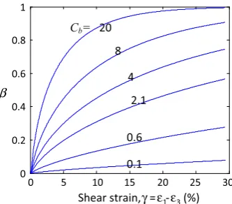
whereCb is a constant controlling the evolution rate ofb. Initially, the soil deforms in a stress state far from the fully yielding stage. As the hardening modulus is very large (i.e. b is small), the material behaves more elastically. Upon further shearing, b increases quickly, and the rate of b reduces rapidly. Whileb¼1; the bounding surface coin-cides with the yield surface. Taking material constants for Toyoura sand listed in Table3, Fig.4 presents example results showing the effect ofCbon the evolution ofbin an initially anisotropic sand sample under undrained shearing. It is evident that a larger value ofCbleads to a higher speed approaching the final state of b¼1. Although this radial mapping law is different from the common method based on interpolations of the hardening modulus (e.g. [8]), it was
shown that these two methods can be equivalently trans-formed into each other [38].
3.6 Effects of shear mode
Results of laboratory tests (e.g. [72, 88] and numerical simulations (e.g. [70,87,93]) demonstrated that the shear mode has a significant influence on the strength and deformation behaviour of granular materials. The shear mode is normally measured by the intermediate stress ratio (b value) or Lode’s angle hl. The relationship between b value andhlis given in Eq. (5). It should be noted that the incorporation of the shear mode effects will remarkably increase the complexity degree of the formulation and numerical implementation.
3.6.1 Effect of shear mode on the critical state
Here the function proposed by Sheng et al. [65] is employed to characterise the relationship between M and Lode’s anglehl:
Mð Þ ¼hl Mcch1ð Þhl ;
h1ð Þ ¼hl
2l4 1 1þl4
1þ 1l 4 1
sin 3hlð Þ !1=4
ð35Þ
wherel1¼Mct=Mcc is a shape parameter;MccandMctare the critical state stress ratios for triaxial compression and extension, respectively. In Eq. (35),h1ð Þhl determines the shape of Mð Þhl in the p plane. For triaxial compression, hl¼ p=6; h1ð Þ ¼hl 1; M¼Mcc; for triaxial extension, hl¼p=6; h1ð Þ ¼h l1; M ¼Mct. According to Loukidis and Salgado [37], the value ofl1is generally in the range of
-0.5 -0.4 -0.3 -0.2 -0.1 0 0.1 0.2 0.3 0.4 0.5 -0.4
-0.3 -0.2 -0.1 0 0.1 0.2 0.3 0.4 0.5 0.6
0 0.1 0.2 0.3 0.4 0.5 0.6 0.7 0.8 0.9 1 -0.4
-0.3 -0.2 -0.1 0 0.1 0.2 0.3 0.4 0.5
0.6 Compression CSL:
CSL: Extension
Critical State Surface Bounding
Surface
Loading Surface
Bounding Surface using stress Lode’s
angle
Loading Surface
Bounding Surface
0
1 p
t
0
1 p
σ
0
2 p
t
0
3 p
t
0
3 p σ
0
2 p
σ
Image Point
Current Point Projection
Normalised mean stress, p/p0
N
o
rm
al
is
ed
s
h
ear
s
tr
e
ss
,
q/
p0
(a) (b)
Fig. 3 Bounding and loading surfaces in the p0-normalised p–q plane and the p plane with cross-anisotropy:
[image:8.595.80.513.481.685.2]0.67–0.75 for silica sands. This shape function is convex for a larger range ofl1 as compared with other kinds of shape function. In particular, the shape function is still convex when l1 is as low as 0.6. If we assume that the critical state friction angles for triaxial extension and compression are equal, Mcc and Mct can be estimated as follows:
Mcc¼
6sinð/cvÞ 3sinð/cvÞ
;Mct¼ 6sinð/cvÞ 3þsinð/cvÞ
ð36Þ
where /cv¼sin1 r1r1þr3r3
c is the critical state frictional angle. Hence,l1 can be expressed in terms ofMcc as:
l1¼ 3 3þMcc
ð37Þ
This relationship was proven to be realistic when com-pared with results of laboratory tests and DEM simulations [95] (e.g. Fig.5). The shape function becomes very similar to that proposed by Matsuoaka and Nakai [39].
A similar shape function is observed for the critical state fabric ratio MF from DEM simulations [81]. The critical state fabric ratioMFis assumed to be a function of Lode’s angle as:
MFð Þ ¼hl MFch2ð Þhl ;
h2ð Þ ¼hl
2l4 2
1þl42þ1l42sin 3hlð Þ !1=4
ð38Þ
where l2¼MFt=MFc, and MFc and MFt are the critical fabric ratios for triaxial compression and extension, respectively. In Eq. (38), h2ðp=6Þ ¼1;MF¼MFc; h2ðp=6Þ ¼l2;MF¼MFt. It is noted that in some DEM simulations under high pressures [44,61,66], the value of MFfor triaxial extension may be even greater than that for triaxial compression. These observations suggest that the shape parameter forMFmight be different from that for the critical state stress ratioM[93].l1andl2in Eq. (38) could be different, and they can be chosen dependently (e.g. a
reciprocal relationshipl1 = 1=l2 [93]) or independently for more general cases. Detailed discussions about the relation betweenl1andl2are out of the scope of this paper.
It is indicated by Eq. (25) that different values ofl1and l2 will lead to a dependency of r0 on the b value as we assumed that the spacing ratioris a constant. Vice versa, a constant r0 means that r is dependent on b value, which further implies that the reference consolidation line and critical state line cannot be independent of the shear mode simultaneously. For simplicity, they are assumed as iden-tical [i.e. Eq. (39)] in the following analysis and model predictions.
l2 ¼l1 ð39Þ
This assumption implies that the proportional coefficient between the critical state stress and fabric ratios, i.e. MF=M¼MFc=Mcc, is a constant.
3.6.2 Effect of shear mode on the yield function
The dependency of M on Lode’s angle makes the yield (loading) function in the p plane not circular. If we gen-eralise the yield surface by using m¼Mð Þhl , the yield surface would be singular atq¼0 (see Fig.3a). To avoid this problem, we replace Lode’s angle hl [i.e. Eq. (6)] in Mð Þhl by another local Lode’s angle h measured from a deviatoric stress tensort¼SSb:
mð Þ ¼h Mcch1ð Þh ;sin 3hð Þ ¼ 3 ffiffiffi 6 p
detð Þt =k kt 3 ð40Þ
After this replacement, we can see that the loading and bounding surfaces are continuous at q¼0 in the p0 -nor-malisedpqplane, and they have the same shape as the critical state surface in thepplane (see Fig.3b). Changes in the fabric anisotropy enable that the yield surface rotates in thepqplane and translates in thepplane. However, the critical state surface is centred at the origin of thepplane, even though an anisotropic critical stress ratio is assumed.
4 8
0.1 0.6 2.1 20
Cb=
Shear strain,γ=ε1-ε3(%) 0
0.2 0.4 0.6 0.8 1
0 5 10 15 20 25 30
β
Fig. 4 Effects ofCbon the evolution of mapping ratiob
0 0.2 0.4 0.6 0.8 1
s1
s2
s3
DEM No effect of
Lode’s angle
( )
1 lh
θ
Fig. 5 Theoretical prediction and DEM results [95] of critical state
[image:9.595.87.254.58.204.2] [image:9.595.340.507.62.213.2]3.6.3 Effect of shear mode on the flow rule
AsMis expressed in terms of Lode’s anglehl in Eq. (35), the stress-dilatancy function defined in Eq. (25) is also dependent on thebvalue.
Considering that the volumetric strain rate is zero at the critical state, the plane strain condition requires that the bvalue of the plastic strain rate at the critical state should be near 0.5. At the critical state, the fabric tensor has the sameb value as the stress tensor. If the flow direction in Eqs. (28) or (29) is applied, thebvalue of the critical state stress tensor under plane strain conditions, denoted asbPSc , should equal 0.5 as well. However, it has been reported (e.g. [88]) that theb value at large strains is between 0.2 and 0.4. Most sands exhibit that the values ofbPS
c are very close to 0.25. This discrepancy suggests that the flow direction may also be dependent on thebvalue. Therefore, the flow directionl0 is expressed by:
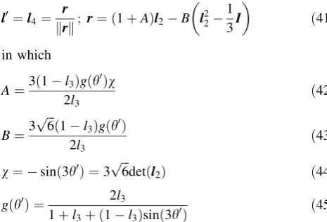
l0¼l4 ¼ r r
k k; r¼ð1þAÞl2B l
2 2
1 3I
ð41Þ
in which
A¼3 1ð l3Þg h 0 ð Þv 2l3
ð42Þ
B¼3 ffiffiffi 6 p
1l3
ð Þgð Þh0 2l3
ð43Þ
v¼ sin 3hð 0Þ ¼3p6ffiffiffidetð Þl2 ð44Þ
gð Þ ¼h0 2l3
1þl3þð1l3Þsin 3hð 0Þ
ð45Þ
wheregð Þh0 is a shape function of the potential function in the deviatoric space. The flow directionl4 is the unit-norm normal of the potential function. When l3¼1, there is gð Þ ¼h0 1; hence, l4¼l2 and the potential function becomes circular in the deviatoric plane [21].
The shape parameter l3 determines the value of bPSc . According to Potts and Gens [55],l3 can be linked to the critical state Lode’s angle for plane strain problems (i.e.hpsc) as follows:
l3¼
sin 3h pscþ1
tanhpscþ3cos 3h psc sin 3h psc1
tanhpscþ3cos 3h psc ð46Þ
Combing with the relationship between bpsc and hpsc in Eq. (5), the relationship between l3 andbpsc can readily be established, as depicted in Fig.6. Whenbps
c is set between 0.2 and 0.4, the value ofl3ranges roughly from 0.7 to 0.9. If such data are not available,bps
c can be taken around 0.25, which corresponds to l3¼0:75. Alternatively, it can be chosen based on available data for sands with similar index properties [37].
3.7 Stress–strain relationship in the rate form
The consistency condition of the loading surface [i.e. Eq. (32)] gives:
_
f ¼fS: _Sþfpp_þfbb_þfp0p_0þfF: _F¼0 ð47Þ
where fS;fp;fb;fp0 and fF are partial derivatives of the loading surface f with respect to S;p;b;p0 and F respectively. The derivatives are detailed in Appendix 1. By inserting the evolution equations with regard to b_;p_0
andF_ into Eq. (47), we can obtain the plastic multiplier as:
_
K¼fS: _Sþfpp_þCF1fF: _g=H ð48Þ
where CF1¼C1ð1þC2k jgjÞ and H is the hardening modulus:
H¼
C3fF: MF
M gF
þfp0ð1þeÞp0
kj
ffiffiffiffiffiffiffiffi 2=3 p
D
fbCblnb
ð49Þ
By substituting the elastic model and flow rule into Eq. (48), the plastic multiplier can be rewritten in terms of total strain rates as:
_
K¼
2G fSð þCF1=pfFÞ: _eþK fpCF1fF:g=p
_
ev Hþ2G fSð þCF1=pfFÞ:l0þ
ffiffiffiffiffiffiffiffi 2=3 p
KD fpCF1=pfF:g
ð50Þ
With the used of Eq. (20), the elastoplastic stress–strain relationship can be written in the rate form as:
_
r¼2Ge_Kl_ 0þK _
evK_pffiffiffiffiffiffiffiffi2=3D
I ð51Þ
00 0.1 0.2 0.3 0.4 0.5 0.6 0.7 0.8 0.9 1
0.05 0.1 0.15 0.2 0.25 0.3 0.35 0.4 0.45 0.5
Shape parameter,l3
ps bc
Fig. 6 Relationship between shape parameterl3 andbps
[image:10.595.50.283.287.445.2]4 Prediction and comparison
Ignoring the potential effects of shearing mode, in total 13 parameters are involved in the new model.MF;C1;C2;C3 represent four newly introduced parameters describing the evolution of the fabric tensor. These four parameters and the initial fabric tensor can be readily determined via regression analysis of relevant microscopic information (e.g. from DEM simulations). However, these parameters are hard to be obtained directly from laboratory tests due to the difficulties in measuring the microscopic structures and their evolution within a soil sample. Alternatively, a trial-and-error method can be used as demonstrated later. Other parameters inherited from CASM_b can be calibrated by the method reported by Yu et al. [91, 92]. If the above effects of the shear mode are considered, two additional shape parametersl1andl3need to be determined.MFand Mshould be interpreted as the corresponding critical fabric values for triaxial compression, i.e.MFC,MCC. In general, l1can be determined by performing conventional triaxial extension tests whenMCCis known, and l3can be deter-mined from plane strain type tests (for example, simple shear test). Alternatively, l1 can be estimated by using Eq. (37), and l3 can be approximately set as 0.75. With given initial values of the stress state, void ratio, and fabric tensor, the initial reference consolidation pressurep0iand the mapping ratio bi can be determined, as shown in Appendix 2.
As aforementioned, the initial fabric tensor and the parameters related to the fabric tensor evolution can be determined directly based on DEM simulation results. Therefore, we first validate the model using the results of DEM simulations in Sect.4.1. Afterwards, comparisons between the model predictions and laboratory test results are presented in Sect.4.2. It needs to point out that the focus will be placed on the performance of the new model in capturing influences of the fabric anisotropy on the shear
strength and non-coaxial flow of granular materials in the following analyses.
4.1 Comparison with DEM simulations
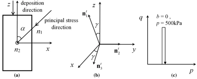
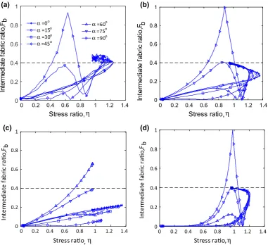
The model is compared with DEM simulations under monotonic shearing with constant mean effective stress p and b value. The DEM tests were carried out by Yang [81] using PFC3D. In the simulations, the samples consist of two-sphere clusters and have highly anisotropic fabric at the initial state due to pre-shearing. The samples were prepared by the deposition method. After isotropic con-solidation to 500 kPa, the samples were pre-sheared tri-axially (i.e. b= 0) up to 10% of shear strain, followed by unloading to an isotropic stress state (see Fig.7c for the pre-loading history). During further monotonic shearing, the mean effective stressp remains constant withb= 0.4, and the direction of the major principal stress is fixed at 0, 15, 30, 45, 60, 75, 90respectively, with respect to the deposition direction (see Fig.7a). Results of the fabric evolution are presented in terms of the fabric deviatorFq -= H3/2kFk, the intermediate fabric ratio Fb= (F2-F3)/ (F1-F3), and the principal direction of the fabric tensor cF(see Fig.7b).Fq,FbandcFgive a complete description of the fabric tensor in a triaxial loading path.
The model parameters for the complete theoretical scheme (SC1) are listed in Table1. It should be noted that in this section possible effects of the shear mode are ignored. HenceMFcandMccare taken as constants and are evaluated atb = 0.4. The fabric tensor after pre-loading is characterised as Fqi¼0:7; Fbi¼0; cFi ¼0. The same initial values of the model parameters for all the simula-tions are taken as follows:
• Initial void ratioei¼0:65;
• Initial fabric tensor Fxxi¼Fyyi¼ 1
3Fqi;Fzzi¼ 2 3Fqi; Fxyi¼Fyzi¼Fxzi¼0;
[image:11.595.102.491.58.215.2]• Initial reference consolidation pressure p0i¼26049kPa;
• Initial value of mapping ratiobi¼0:0269.
In addition, three additional theoretical schemes as summarised in Table2are also applied for the comparison analysis. The theoretical scheme 2 (SC2) using the flow direction of Eq. (28) is to more clearly reveal the effects of associativity of flow rule in the deviatoric space. All the material constants used in SC2 are the same as those in
[image:12.595.51.543.73.109.2]SC1. In order to examine the influence of the fabric evo-lution law on the predicted stress–strain relations, model predictions with the evolution laws in Eqs. (15) and (16), respectively, are also performed. Material constants used in SC3 and SC4 are the same as those used in SC1. The initial values are identical in all theoretical schemes.
Table 1 Material constants of the DEM samples
k v k M U C
b Cd r0 n C1 C2 C3 MF
[image:12.595.61.547.147.197.2]0.005 0.3 0.058 0.95 2.13 10 1.5 50 2 0.32 1.3 9 1
Table 2 Summary of theoretical schemes
SC1 SC2 SC3 SC4
Evolution law Equation (14) Equation (14) Equation (15) Equation (16)
Flow rule in the deviatoric space Equation (29) Equation (28) Equation (29) Equation (29)
Fabric deviator,F
q
0 0.2 0.4 0.6 0.8 1 1.2 1.4 1.6
α=0o
α=15o
α=30o
α=45o
α=60o
α=75o
α=90o (a)
Stress ratio,η Stress ratio,
0 0.2 0.4 0.6 0.8 1 1.2 1.4 1.6
Fabric deviator
,F q
η
(b)
0 0.2 0.4 0.6 0.8 1 1.2 1.4
0 0.2 0.4 0.6 0.8 1 1.2 1.4 0 0.2 0.4 0.6 0.8 1 1.2 1.4
Fabric deviator
,F q
Stress rao ,η
0 0.2 0.4 0.6 0.8 1 1.2 1.4 1.6 (c)
0 0.2 0.4 0.6 0.8 1 1.2 1.4
0
Fabric deviator
,F q
Stress rao ,η
0.2 0.4 0.6 0.8 1 1.2 1.4 1.6 (d)
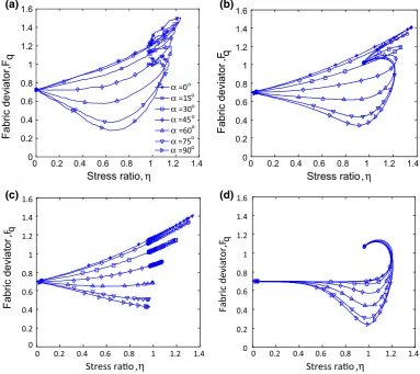
[image:12.595.106.490.356.697.2]4.1.1 Fabric evolution
Figures8, 9 and 10 show results of the fabric evolution obtained from both DEM simulations and model predic-tions in terms of the fabric deviatorFq, intermediate fabric ratioFb, and principal fabric directioncF, respectively. At large strains, DEM results under various loading directions show that:
• the intermediate fabric ratio Fb evolves towards the intermediate stress ratio, i.e.Fb¼b¼0:4;
• the principal fabric direction cF evolves towards the principal direction of stress tensor; hence, the fabric tensor becomes coaxial with the stress tensor;
• the fabric deviatorFqevolves towards a unique value of Fq ¼MF¼1.
Therefore, the fabric tensor tends to evolve towards a unique critical fabric tensorFc, which is independent of the loading direction. This behaviour was also observed in other DEM simulations with different initial fabric tensors (e.g. [82, 95]). If we set the coordinate system coincident with the loading directions, initial components of the fabric
tensors in the new coordinate system may vary with the loading direction. In other words, the unique critical fabric tensor is essentially independent of the initial fabric ten-sors. The critical state fabric tensor is proportional to the critical state stress tensor as postulated in Eq. (13). When a45,Fqwill increase to a peak value and then decreases gradually to the critical state valueMF¼1; whena[45
, Fq will decrease initially to a minimum value, increase gradually afterwards to a peak value and then decrease again to the critical state value.
All these features of the fabric evolution are well cap-tured by SC1 [namely, while using the fabric evolution law of Eq. (14)]. The only imperfection in the predictions of Eq. (14) is thatFqconverges toMF¼1 more quickly than the DEM simulation results whilea45. This may be due to that the chosen value of parameterC3is slightly large. A smaller value of C3 will ensure that the fabric evolution approaches the critical state slower. The fabric evolution predicted by SC2 (not presented here for brevity) is almost the same as those by SC1. It implies that the flow direction does not exert a significant effect on fabric evolution. This is consistent with the fact that the fabric evolution law (14)
In
te
rm
ed
ia
te
fa
b
ri
c
ra
ti
o
,Fb
0 0.2 0.4 0.6 0.8 1
α=0o
α=15o
α=30o
α=45o
α=60o
α=75o
α=90o (a)
Stress ratio,η
0 0.2 0.4 0.6 0.8 1
In
te
rm
e
di
at
e f
a
br
ic
r
a
ti
o
,F b
Stress ratio,η
(b)
0 0.2 0.4 0.6 0.8 1
Stress rao,η
In
te
rm
ed
iat
e f
ab
ric
r
ao
,Fb (c)
0 0.2 0.4 0.6 0.8 1 1.2 1.4
In
te
rm
ed
iat
e f
ab
ric
r
ao
,Fb
Stress rao,η
0 0.2 0.4 0.6 0.8 1 (d)
0 0.2 0.4 0.6 0.8 1 1.2 1.4
0 0.2 0.4 0.6 0.8 1 1.2 1.4 0 0.2 0.4 0.6 0.8 1 1.2 1.4
[image:13.595.108.490.58.406.2]is dependent only on the norm, rather than the direction, of the deviatoric plastic strain rate. SC3 can capture the fabric evolution at a low stress level, but it has poor performance at large strains as the predicted fabric tensors do not gen-erally evolve towards the critical state fabric tensor. SC3 performs relatively better when the angle of the loading direction is small. SC4 can capture the critical state char-acteristics of the fabric tensor but does not perform well at the pre-softening stage. This is due to that the plastic strain rate is very small before the peak stress ratio, and the fabric hardly evolves according to the fabric evolution law (16) at this stage.
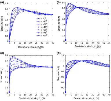
4.1.2 Strength and volumetric response
Figures11 and 12 present DEM simulation results and model predictions of the stress ratio and the volumetric strain under different loading directions. Not surprisingly that SC1 gives best predictions of the stress–strain beha-viour over the entire loading paths. With increases of the loading direction angle, the peak strength decreases and the shear strain required to mobilise the peak strength increases.
The response of the sample is softer and more contractive in tests with a larger loading direction angle. At large shear strains, both the stress ratio and void ratio evolve towards a unique value. SC3 captures the trend of the effects of loading direction on the peak strength, but it fails to predict a unique void ratio for tests with different loading direc-tions. This can be explained by the fact that SC3 cannot predict a unique fabric tensor at large strains. After the peak stress ratio, the fabric tensor predicted by SC3 obviously deviates from DEM results. The performance of SC3 is better for a small loading direction angle. SC4 captures the volumetric deformation behaviour satisfactorily, but it fails to predict the effects of loading direction on the peak strength. The comparison of results predicted using differ-ent flow rules in the deviatoric space (i.e. SC1 and SC2) shows that the flow direction has an insignificant effect on the stress ratio and the volumetric strain.
4.1.3 Fabric anisotropy and non-coaxiality
Figure13presents DEM simulation results and theoretical predictions of principal directions of the total strain 0
0.2 0.4 0.6 0.8 1 1.2 1.4
0 15 30 45 60 75 90
α=0o
α=15o
α=30o
α=45o
α=60o
α=75o
α=90o (a)
o
Principal fabric direcon, F( )γ
St
re
ss
r
a
o,
η
0 0.2 0.4 0.6 0.8 1 1.2 1.4
St
re
ss
r
a
o,
η
15 30 45 60 75 90
15 30 45 60 75 90
Principal fabric direcon,γF(o)
(b)
0 0.2 0.4 0.6 0.8 1 1.2 1.4
0
St
re
ss
r
a
o,
η
o
Principal fabric direcon,γF( )
(c)
0 15 30 45 60 75 90
0 0.2 0.4 0.6 0.8
1
1.2 1.4
St
re
ss
r
a
o,
η
o
Principal fabric direcon, F( )γ
[image:14.595.108.490.62.399.2](d)
increment (diamond) and the plastic strain increment (cir-cle), in reference to the principal direction of the stresses. As it is not easy to distinguish the elastic strain increment from the total strain increment in DEM results, only results of the total strain increment are presented. Generally, the value of the non-coaxial angle increases with an increase in the loading direction angle fora ranging from 0 to 45, and decreases are shown with further increases of the loading direction whilea is larger than 45. At 0and 90
directions, the total strain increment is coaxial with the stress tensor, which is due to that the fabric tensor is coaxial with the stress tensor, as shown in Fig.10. While the loading direction varying between 0and 90, the non-coaxial angle will reduce to zero gradually after the peak stress ratio as the fabric tensor evolves towards the critical state at which the fabric tensor is coaxial with the stress tensor. All these features are captured by SC1 and SC2 in terms of the total strain increments. However, the predic-tions of SC1 and SC2 are different in terms of the plastic strain increments. When the stress ratio is low, the pre-dicted principal directions of the plastic strain increments by SC2 are unrealistically large in comparison with those
by SC1. In theoretical predictions, at a low stress ratio the total strain increment is nearly coaxial with the stress even though the principal direction of the plastic strain obvi-ously deviates from that of the stress tensor. Considering that the elastic strain increment is always coaxial with the stress tensor as an isotropic elastic model is assumed, it can be inferred that the plastic strain develops gradually and is smaller than the elastic strain at a low stress ratio. How-ever, the DEM simulation results show that even at a very low stress ratio, the strain increment is non-coaxial with the stress tensor. This may imply that the elastic behaviour is also anisotropic or the plastic strain increment should be larger than the predicted values by SC1 and SC2. As the stress ratio increases, predicted principal directions of the total strain increment and plastic strain increment become coincident, which implies that the elastic strain increment becomes ignorable when compared with the plastic strain increment. SC3 and SC4 adopt the same flow rule as SC1, but SC3 is not able to predict coaxial deformation at large strains as the fabric tensor cannot evolve to be coaxial with the stress tensor. Overall, from the comparison, it can be concluded that deformation non-coaxiality is highly related
(a)
0 0.2 0.4 0.6 0.8 1 1.2 1.4
Deviatoric strain,εq(%)
St
re
ss
r
a
o,
η
0 5 10 15 20 25 30 35 40
0 5 10 15 20 25 30 35 40 0 5 10 15 20 25 30 35 40
α=0o
α=15o
α=30o
α=45o
α=60o
α=75o
α=90o
0 5 10 15 20 25 30 35 40
Deviatoric strain,εq(%)
St
re
ss
r
a
o,
η
0 0.2 0.4 0.6 0.8 1 1.2 1.4
(b)
St
re
ss
r
a
o,
η
Deviatoric strain,εq (%)
0 0.2 0.4 0.6 0.8 1 1.2 1.4
(c)
St
re
ss
r
a
o,
η
Deviatoric strain,εq (%)
0 0.2 0.4 0.6 0.8 1 1.2 1.4
[image:15.595.107.491.57.406.2](d)
to fabric evolution and is significantly influenced by the flow rule in the deviatoric space.
4.2 Comparison with laboratory tests
The applicability of the model is further assessed by comparing with experimental results in the literature. Model predictions for tests on different sands with various loading paths under both drained and undrained conditions are performed.
A series of tests investigating the drained behaviour of air-pluviated Leighton Buzzard sand (Faction B) have been performed by Yang [80]. The maximum and minimum void ratios of the sand are 0.79 and 0.52, respectively. The specific gravityGs is 2.65. Only limited test results were reported for the Faction B Leighton Buzzard sand. As Portaway sand has index properties very similar to this sand, the elastic and critical state parameters are taken as suggested by Yu et al. [91] for Portaway sand (Gs¼2:65;emin¼0:46;emax¼0:79). The dilatancy parameterCdis calibrated using the response between the volumetric strain and the shear strain in triaxial compres-sion tests. The spacing ratioris estimated by assuming the
maximum state parameter equals 0.07, which is also close to the value calibrated for Portaway sand (i.e. 0.06).
Model predictions are also compared experimental results from drained true triaxial tests [40] and simple shear tests [56] and undrained true triaxial and simple shear tests [88] with Toyoura standard sand. For Toyoura sand, the elastic parameters follow those suggested by Gutierrez and Ishihara [16], and the critical state parameters are deter-mined from the data reported by Verdugo and Ishihara [74], as shown in Fig.1. Parameters Mcc and l1 are obtained from the test results andl3is determined asbpsc ¼ 0:25 from simple shear tests at large strains as reported by Yoshimine et al. [88]. The spacing ratioris determined by assuming that the maximum state parameter equals 0.1. The dilatancy coefficientCdis taken from Miura and Toki [40].
The initial fabric tensor and the model parameters related to the fabric evolution are optimised through trial-and-error with reference to the values calibrated from the previous DEM simulations. The material parameters for both sands are summarised in Table3. It is reasonable to assume that the initial fabric tensor is cross-anisotropic, namely Fb¼0. Initial values of the fabric deviator for
-10
-8
-6
-4
-2
0
2
α=0o
α=15o
α=30o
α=45o
α=60o
α=75o
α=90o
Deviatoric strain,εq(%)
V
o
lu
m
et
ric
s
tr
ain
,
εv
(%
)
(a)
0 5 10 15 20 25 30 35 40 0 5 10 15 20 25 30 35 40
-10
-8
-6
-4
-2
0
2
ε
α=0o
α=15o
α=30o
α=45o
α=60o
α=75o
α=90o
V
o
lu
m
et
ric
s
tr
ain
,
εv
(%
)
(b)
Deviatoric strain, q(%)
0 5 10 15 20 25 30 35 40
Deviatoric strain,εq(%)
V
o
lu
m
et
ric
s
tr
ain
,
εv
(%
)
-10
-8
-6
-4
-2
0
2
(c)
Deviatoric strain,εq (%)
0 5 10 15 20 25 30 35 40
-10
-8
-6
-4
-2
0
2
ε
Vo
lu
m
et
ri
c s
tr
ai
n
,v(%
)
[image:16.595.108.489.57.399.2](d)
Leighton Buzzard sand and Toyoura sand are set as 0.375 and 0.488, respectively. In all of the following predictions, the influence ofb value is considered.
4.2.1 Drained behaviour of Leighton Buzzard sand
Figures14, 15, 16 and 17 compare test data and model predictions for air-pluviated Leighton Buzzard sand under monotonic shearing with constant values ofbanda. In all
these tests, the mean stress was kept constant at 200 kPa. The loading condition and test setups were elaborated by Yang [80]. Overall, the constitutive model generally captures the influences of the loading direction and the b value on the drained behaviour of Leighton Buzzard sand. In general, an increase of either the angleaor thebvalue may lead to lower shear strength and more contractive behaviour.
It is shown that before the peak strength is mobilised (typically when the shear strain is lower than 10%), the
0 15 30 45 60 75 90
0 0.2 0.4 0.6 0.8 1 1.2 1.4
Principal direcon (o)
St
re
ss
r
a
o,
η
(a)
S
tre
s
s
ra
ti
o
,
η
Principal direcon (o)
(b)
0 0.2 0.4 0.6 0.8 1 1.2 1.4
0 15 30 45 60 75 90
0 15 30 45 60 75 90
0 0.2 0.4 0.6 0.8 1 1.2
Principal direcon(o)
η
S
tr
e
ss r
a
ti
o
,
(c)
Principal direcon (o)
0 15 30 45 60 75 90
St
re
ss
r
a
o,
η
0 0.2 0.4 0.6 0.8 1 1.2 1.4 (d)
0 15 30 45 60 75 90
St
re
ss
r
a
o,
η
Principal direcon (o)
[image:17.595.107.491.59.562.2]0 0.2 0.4 0.6 0.8 1 1.2 1.4 (e)
predicted strength and volumetric response are in good agreement with the test results; after that, the predicted sand response is stiffer and more dilative than that mea-sured in the tests for most cases. These differences may be attributed to the fact that after the peak stress ratio shear bands develop quickly and become obviously visible, which leads to high hetero-homogeneity of the hollow
[image:18.595.50.290.72.398.2]cylindrical samples in the laboratory tests (see Fig.18a). Consequently, the hetero-homogeneity prevents the fabric evolution towards the unique critical state fabric in the tests. However, a unique critical state fabric is assumed in the constitutive model, and the model parameters related to fabric evolution were determined with reference to the DEM results. In the DEM simulations, the sample is homogenous and no shear band can be observed even at very large shear strains (see Fig.18b). In the DEM simu-lations, the sample is not in a cylindrical shape but as a solid drum, and a new technique is used to control the movement of planes for generating general loading paths. The use of this technique maintains that the sample tends to be macroscopically uniform even at a large shear strain (e.g. eq ¼40%). Besides, the particle number used in the DEM simulations is limited when compared with that involved in laboratory tests. This may also inhibit the macroscopic development of shear bands, even though micro-shear bands of several particle diameters in width could develop. For example, in Fig.14, the experimental results obtained from tests with different loading directions show no sign of a unique critical stress ratio or a unique void ratio to be reached at the critical state. In the model predictions, however, the volumetric strain and the stress ratio continuously evolve towards the same value as the fabric evolves towards a unique anisotropic critical state. In addition, the discrepancy between the predicted and measured volumetric strains (e.g. the case ofb¼1;a¼0 in Fig.15) suggests that the dilatancy function is dependent on the current fabric. Although it may increase the degree of complexity of the model, additional assumptions about the dependency of the dilatancy function on the fabric tensor need to be introduced, which can further improve the accuracy of the model prediction on the volumetric deformation response.
Table 3 Summary of material parameters
Category Symbol Leighton Buzzard sand (Faction B)
Toyoura sand
Remarks
Elasticity k 0.005 0.004 Typical value used
m 0.16 0.2
Critical state
k 0.025 0.031 Figure1
C 1.800 2.067
Mcc 1.16 1.25 Triaxial
compression tests
MFc 1 1 Assumed
Yield surface
r=r0 33/3568 40.6/ 3130
Estimated by the maximum state parameter
n 2 2 Typical value
used
Dilatancy Cd 0.85 0.9 Triaxial tests
Mapping law
Cb 5 0.65 Trial-and-error
Fabric evolution law
C1 0.37 0.38 Trial-and-error
C2 1.3 1.3
C3 5.2 4.5
Effect of bvalue
l1 0.73 0.75 Triaxial
extension tests
l3 0.75 0.75 Plane strain
tests
Predicted Measured
b=0.5 p=200kPa
α=0o
α=30o
α=90o
α=0o
α=30o
α=90o
St
re
ss
r
a
o,
η
Deviatoric strain,εq (%)
0 5 10 15 20
0 0.2 0.4 0.6 0.8 1 1.2 1.4 1.6
(a)
0 5 10 15 20
Deviatoric strain,εq (%) 2
1 0 -1 -2 -3 -4 -5 -6
V
o
lu
m
et
ric
s
tr
ain
,
εv(%
)
[image:18.595.112.490.519.683.2](b)
Fig. 14 Comparison between model predictions and measured data for drained shear tests of air-pluviated Leighton Buzzard sand (Faction B)
4.2.2 Undrained true triaxial tests of Toyoura sand
Figures19 and 20 compare model predictions and mea-sured results [88] for dry-deposited Toyoura sands in undrained shear tests with different loading directions and bvalues. It is shown that the model satisfactorily predicts
the influences of the loading direction and the intermediate stress ratio as well as the relative density on the undrained behaviour of Toyoura sand. It shows that a larger value ofa or b generally leads to a softer and relatively more con-tractive sand response, which is also often observed in tests under drained conditions. It is noted that the model cap-tures the gradual exhibition of the existence of the ‘quasi-steady state’ with an increasing value of the loading angle. It also predicts the gradual recovery of the shear stress after the ‘quasi-steady state’. However, the model predictions show that the recovery of shear stress after the ‘quasi-steady state’ ata 45 is slower than that of the measured data for samples ofDr= 39–41%, but faster than that for samples ofDr= 31–34%.
4.2.3 Undrained torsional simple shear test of Toyoura sand
Figure21shows a comparison between the model predic-tion and the measured data in undrained torsional simple shear tests of dry-deposited Toyoura sand [88]. The sample was torsionally sheared from an initial anisotropic con-solidation state with p¼133kPa and q¼100kPa. As shown in Fig.21, the model predicts the sand response reasonably well in the case ofe0¼0:835. When shearing begins, the direction of the major principal stress rotates rapidly to the direction a¼45 and the bvalue increases quickly towardsb¼0:25. Although the model predicts the measured data in trend for the case ofe0¼0:858, the shear stress recovers quicker than that measured. This may be due to that the realistic critical state line in the vlnp plane is nonlinear (the slope of the critical state line decreases with an increasing void ratio). After the ‘quasi-steady state’, stresses evolve towards the critical state values, but the linear assumption for the critical state line b=0.2
b=0.5 b=1
b=0.2 b=0.5 b=1
Measured Predicted
α=0o p=200kPa
0 5 10 15 20
0 0.2 0.4 0.6 0.8
1
1.2 1.4 1.6
St
re
ss
r
a
o,
η
Deviatoric strain,εq (%)
(a)
0 5 10 15 20
Deviatoric strain,εq (%)
2 1 0 -1 -2 -3 -4 -5 -6
V
o
lu
m
et
ric
s
tr
ain
,
εv(%
)
[image:19.595.109.490.60.230.2](b)
Fig. 15 Comparison between model predictions and measured data for drained shear tests of air-pluviated Leighton Buzzard sand (Faction B)
with differentbvalues ata¼0.aDeviatoric strain vs. stress ratio;bdeviatoric strain vs. volumetric strain
Deviatoric strain,εq (%)
St
re
ss
r
a
o,
η
0 0.2 0.4 0.6 0.8 1 1.2 1.4 1.6
0 5 10 15 20
0 5 10 15 20
=30o
α
b=0.2 b=0.5 b=1
b=0.2 b=0.5 b=1
Measured Predicted
p=200kPa
(a)
2 1 0 -1 -2 -3 -4 -5 -6
Deviatoric strain,εq (%)
v
Vo
lu
m
et
ri
c s
tr
ai
n
,
ε
(%
)
(b)
Fig. 16 Comparison between model predictions and measured data
[image:19.595.86.254.278.578.2]in the vlnp plane overestimates the critical state shear stress, which makes the predicted recovery of the shear stress faster than that measured in the tests with loose sand samples.
4.2.4 Drained triaxial test of Toyoura sand
Figure22 presents a comparison between the model pre-dictions and the measured data for drained shear tests on Toyoura sand samples prepared by a multiple sieving pluviation method. Although different preparation methods might induce different initial fabrics in a sample [53], the initial fabric deviator was estimated based on dry-deposited sand samples because of the insufficient relevant
information in the source reference. Fq¼0:485 is used in the predictions given in Fig.22. Despite that the stiffness and the dilation response of the sand are slightly overes-timated, the influence of the loading angle on the drained behaviour of Toyoura sand is well captured by the model.
4.2.5 Drained simple shear test of Toyoura sand
Figure23shows predicted and measured results of drained simple shear tests that performed on air-pluviated Toyoura sand samples with different initial void ratios [56]. Prior to performing shear tests, the samples were one-dimension-ally consolidated until the vertical stress r11¼98kPa was reached. During shearing, the vertical stress was kept
Stress rao
,
η
0 0.2 0.4 0.6 0.8 1 1.2 1.4
Deviatoric strain,εq (%)
10 15 20
=90o α
b=0.2 b=0.5 b=1
b=0.2 b=0.5 b=1
Measured Predicted
p=200kPa (a)
Deviatoric strain,εq (%)
Volumetric strain,
εv(%)
1 0.5 0 -0.5 -1 -1.5 -2
0 5 0 5 10 15 20
[image:20.595.106.492.280.501.2](b)
Fig. 17 Comparison between model predictions and measured data for drained shear tests of air-pluviated Leighton Buzzard sand (Faction B)
with differentbvalues ata¼90.aDeviatoric strain vs. stress ratio;bdeviatoric strain vs volumetric strain
Fig. 18 Typical sample shapes at a large shear strain.alaboratory tests with obvious shear bands (after [80]);bDEM tests without obvious shear