Finite algorithms for linear optimisation problems

LINEAR OPTIMISATION PROBLEMS

by

Va.vid I .

ce.aJtk.

A thesis submitted to the Australian National University for the degree of Doctor of Philosophy

(i)

ACKNOWLEDGEMENTS

The work for this thesis was carried out at the Computing Research Group and the Department of Statistics, I.A.S., Australian National University. I gratefully acknowledge the financial assistance of the Australian National University during this time.

I am indebted to Mike Osborne for his help and supervision of my work .and for his constructive conunents on the· draft of this thesis. I would also like to thank Robin Stanton for helpful.

conversations and David Anderson in providing test programs for the L

1 algorithm, and members of the Computing Research Group and the Department of Statistics for a congenial and constructive work

environment.

Thanks are also due to the typist, Mrs. Susan Watson, for care and tolerance at a difficult time, and to my mother, Cherrie, and my wife, Mel, for conscientious proof-reading.

PREFACE

Some of the work of this thesis was carried out in

collaboration with Dr. Michael Osborne. In particular, Chapters 3 and 5 contain results which were established jointly. Also, Chapters 2 and 3 have been published as Clark (1980) and Clark and Osborne

(1980) respectively.

ABSTRACT

In this thesis we investigate certain linear optimisation problems,

. . .

minimise f(x) subject to

where the Kuhn-Tucker conditions

(i) g. (x) ~

i - 0 i = 1, ... , n (ii) for some u ~ ₀ 'vf(x)

(iii) u g (x) T = 0

-

-g. (x) ~ 0 , i

-= Lu.'vg. (x) l i ~

comprise a set of simultaneous linear equations.

i = l, ... ,n

Chapter 1 introduces the problems, the restricted least squares (RLS), M-estimator, and least absolute deviations (LAD) problems, and places them in their context.

(iii)

In Chapter 2, the RLS problem is examined, and pruning

rules developed which transfonn a rather inefficient branch and bound algorithm into an essentially iterative one. The implementation of the resulting algorithm is considered in Chapter 3 and, by working

with dual variables and using orthogonal transformations, the algorithm -in its f-inal form is at least competitive with existing algorithms for this problem. An error analysis is also given, showing that the use of dual variables has led to superior numerical properties.

proving a theorem. The broad areas covered by these speculations include the question of non-uniqueness, the connection between the M-estimator and the LAD estimator, what might be called the "proper

behaviour" of the function and the function value itself.

Chapter 5 deals with algorithms for calculating the M-estimator. Existing algorithms are surveyed, and two new ones developed. One of them, a continuation algorithm, is examined in detail and numerical results presented. Finiteness is proved for

them both.

Finally, in Chapter 6, the LAD problem is considered. The existing algorithms are reviewed and a new one presented which,

although proven finite, did not perform competitively on a particular class of example . The thesis concludes with a discussion of why the algorithm failed, how it differs from algorithms which succeeded for

ACKNOWLEDGEMENTS PREFACE

ABSTRACT

TABLE

OF

CONTENTS

CllJ\PTER 1: TllE PROBLEMS INTRODUCED

CHAPTER 2: AN ALGORITI-IM FOR THE RESTRICTED LEAST SQUARES PROBLEM

2.1 INTRODUCTION

Page (i) (ii) (iii) 1 6 6 2.1 .1 The constrained least squares problem 6 2.1.2 The restricted least squares problem 8

2.1 .3 Notation 10

2.1.4 Branch and bound 10

2.2 THE NEW ALGORITHM

2.2.1 The Armstrong and Frome algorithm 2.2.2 Improved prW1ing rule

2.2.3 Optimality conditions

2.2.4 Selection of the next node 2.2.S The algorithm sununarised

2. 3 COMPLEXITY 2. 4 RESULTS

2.5 EXTENSION TO OTHER PROBLEMS 2.6 CONCLUSION

CHAPTER 3: AN EFFICIENT I~WLE!v!ENTATION OF THE LEAST SQUARES ALGORITHM

3.1 INTRODUCTION

3.2 USE OF ORTHOGONAL TRANSFORMATIONS 3.3 NUMERICAL RESULTS

CHAPTER 4: 4.1

THEM-ESTIMATOR: STRUCTURE INTRODUCTION

4.1.l Robust estimation and the rejection of

11 11 11 15 17 20 21 23 23 25 27 27 30 35 40 40

outliers 40

·---.-

4111

4.2

4.3

4.4

DEFI ITIONS AND PREAMBLE

4.2.1 Definitions and conventions

4.2.2 Preamble

SPECULATIONS AND EXAMPLES

4.3.l On tightness and non-uniqueness

4.3.2 On the function value of feasible partitions

4.3.3 On the value of the AD function at feasible partitions

4.3.4 On the signs of residuals at change of

Page 43 43 45 46 46 47 47

partition 48

4.3.5 On the feasibility of residuals at change

of partition 48

4.3.6 On non-uniqueness and connectedness 49 4.3.7 On o , as c varies

4.3.8

4.3.9

On 0

C and 00

More on tightness and non-uniqueness

4.3 .10 On oc and o

0 , for small c

50

so

51

52

4.3.11 On non-uniqueness of LAD and M-estimators 52

RESULTS 53

4.4.1 On tightness and non-uniqueness 56 4.4.2 On function values of feasible partitions 60 4.4.3 On signs and values of residuals in

non-unique partitions 61

4.4.4 On the size of residuals at change of partition

4.4.5 On the composition of o and

o

4.4.6 On the size of o

64 65

66

4.4.7 On the connection with LAD for small c 66

4.5 SUMMARY 68

CHAPTER 5: AN ALGORITHM FOR THEM-ESTIMATOR 5.1 VARIOUS APPROACHES

5.2 THE ALGORITHM

69

69

72

5.2.1 Piecewise linearity 72

5.2.2 Updating at change of partition 73 5.2.3 The choice of orthogonal transformation 76 5.2.4 Behaviour of derivatives at change of

partition 79

--5.2.5 The algorithm summarised

5.3 FINITENESS

5.4 NUMERICAL RESULTS 5.5 M-ESTIMATOR DUALITY

5.5.1 LP duality

5.5.2 M-estimator duality

CHAPTER 6: AN ALGORITHM FOR THE LEAST ABSOLUTE DEVIATIONS ESTIMATOR

6.1 INTRODUCTION 6.2 THE ALGORITHM

6.2.1 General description

6.2.2 Updating at change of partition 6.2.3 Progress of the algorithm

6.2.4 The algorithm summarised 6.3 REFINEMENTS TO THE ALGORITHM 6.4 FINITENESS

6.5 NUMERICAL RESULTS AND DISCUSSION

BIBLIOGRAPHY

Page

79 80 88 90 90 91

93 93

95 95 103 106 109 109 112 115

(1. 1)

CHAPTER 1

THE PROBLEMS INTRODUCED

For the general mathematical programming problem

. . .

minimise f(x) subject to g. (x) ~ 0

i -

'

i = l, ...

,n,

*

the well-known Kuhn-Tucker conditions for a stationary point at x are

*

(1. 2) g. (x ) ~ 0 i

-i = 1, ... ,n

*

*

(1.3) for some u ~ 0 , 'vf(x) = I:u.'vg. (x ) i i

-(1. 4) u T g (x ) * = 0 .

If (1.2) to (1.4), which characterise a local optimum, comprise a set of linear equations, the problem is a linear

optimisation problem (LOP). LOPs have interest and importance in their own right, in forms as diverse as standard linear programming, quadratic programming, and matching problems. Provided (1.2) to

non-linear, cutting plane methods still solve an LOP at each step

(eg, Luenberger, 1973).

It is worth noting that although general methods may exist for a class of problems, it is often the case that a particular

2.

member of the class is so structured that a close examination of the problem yields a much simpler method of solution. Well-known examples of this are geometric programming, (Duffin, Peterson and Zener, 1967) '· where a particularly vile-looking non-linear optimisation problem can be transformed into an LOP, and the transportation problem, (eg, Hadley, 1962) where an LOP can be solved simply without recourse to more

general techniques, such as the simplex method.

The problems studied 1n this thesis, the restricted least squares (RLS), M-estimator, and least absolute deviation (LAD)

problems all display this feature, where a close examination of the problem leads to a method of solution which is able to take advantage

of the structure of the problem so that an algorithm can be tailored to fit it expressly. This is clearly illustrated by the RLS problem,

(Chapter 2) where, starting from a general branch and bound search algorithm, analysis of the problem leads to a vastly reduced search-tree, and then further analysis leads to a finite iterative algorithm far superior to the original search algorithm. Further analysis still

(Chapter 3) then in<licatcs an efficient method of implementation of the algorithm which test results have shown to be more than

competitive with standard linear programming techniques, and which has the added ~dvontagc of superior numerical properties.

The RLS problem is important both in its own right, and because it forms a central step in many algorithms for more general

LOPs, and as such has received a great deal of attention~ Typical of the linear-programming based algorithms written specifically for the RLS problem is that of Lawson and Hanson (1974). The overall scheme of their algorithm is to start from an initial primal feasible solution (x= 0) , and at each step maintain both primal feasibility

and complimentary slackness, terminating when dual feasibility is also

achieved. The other approach which has been tried on this problem is

to place it in a branch and bound framework. Armstrong and Frome's

algorithm (1976) using this technique is not competitive for large

problems, and does not appear promising, yet successive refinements

of it resulted in a competitive stable algorithm, similar in some

ways to the linear-programming based algorithms, but differing from

them in that only complimentary slackness is preserved at each

iteration, the direction of the algorithm being towards finding a

dual feasible point and then testing it for primal feasibility.

The M-estimator is one of a number of statistical measures

which have been suggested in an effort to minimise the effect of and

identify outlying observations . Although interest in rejection

criteria stems back at least one liundred years (eg). Peirce, 1852), the current surge of interest in the so-called robust estimators was

catalysed by Tukey in 1960 when he showed that the widely used least

squares estimator was 1n some ways inferior to the least absolute *

deviation estimator. Strictly speaking, if x minimises .

.

.

*

Ep(/\x.-b.) for some function p , then x

- i i 1s a maximum-likelihoo<l

or M-estimator for the linear model b = Ax - E under some appropriate assumption of distribution of E • The most commonly used function p,

(1. 5) p(t) =

\t

2

=

cltl

\c

2

$ C

> C •

4.

One of the thrusts of this thesis has been to examine the

problems carefully in an effort to understand their underlying

structure, and probably the major contribution has been the examination

of the M-estimator when detailed properties of it are given for the

first time. In particular, the relationship between the M-estimator

and the LAD estimator is explored, and the question of uniqueness

thoroughly examined. Although several of the theorems developed do

not have a direct bearing on algorithm development, two algorithms

arise fairly naturally from the study and an understanding of the

structure has facilitated proving finiteness for them.

Another area which has experienced a resurgence of interest

due to the interest in robust estimation has been least absolute

deviation regression. Used in line-fitting models, it predates

the least squares method, being used by Boscovitch in 1757, but it

was not until 1973 that an efficient algorithm was written by Barrodale

and Roberts. Since then several efficient algorithms based on either

the simplex method or a gradient method have been developed. A feature

of all these algorithms is that they have a full basis at each step,

and have been shown by Osborne, 1980, to be in a sense identical. The

algorithm presented in this thesis does not necessarily work with

a full basis. It is not yet clear how the increased freedom in choice

of descent direction should be used, and in its current form the

algorithm is not always competitive, but even the failure of the

A final point is that although the nature of this approach,

of studying the structure of the problem, of necessity leads to an

algorithm specifically tailored to a particular problem, the approach

of an algorithm is not necessarily confined to its own problem. Thus

the first algorithm for the M-estimator is the progenitor of that for

the LAD estimator, and the approach developed there can be fairly

directly applied to solving other LOP problems, and the RLS algorithm

2.1

2.1.1

CHAPTER 2

AN ALGORITHM FOR THE RESTRICTED LEAST SQUARES PROBLEM

INTRODUCTION

The Constrained Least Squares Problem

With its wide applicability, the constrained least squares

problem (CLSP)

(2.1) m1n1m1se . . .

subject to Ex=

f

Gx ~ h

has received a great deal of attention. In its equivalent form,

(2.2) m1n1m1se

subject to

T T T

x Cx + c x + d d Ex= f

Gx ~ b

6.

it 1s a convex quadratic programming problem, and early algorithms to

solve the problem used quadratic programming techniques based on the

simplex algorithm (see, eg, Cottle 1968, Cottle and Danzig 1968,

Lemke 1968, Wolfe 1959). However, these methods, based on pivoting

and inverse basis techniques, have been found to be numerically

unstable (see, eg, Wilkinson 1961, 1965, Golub and Wilkinson 1966).

Moreover, as shown by Golub 1965, and Golub and Saunders 1969, the

problem in its second form (2.2) is always more ill-conditioned than

in its first form (1.2).

For these reasons, a number of algorithms have been developed

decomposition, as do Bartels, Golub and Saunders 1970, whilst Lawson and Hanson 1974, (cited by Bartels, 1975, as the definitive handbook on Least Squares problems) use a Q-R decomposition. The numerical properties of the two decompositions are similar. It should be emphasised that the chief aim of these methods is to improve the

numerical stability of the algorithm, and that any improved efficiency (as reported, eg, by Osborne, 1976) is a pleasing side-benefit.

It is instructive to examine the algorithms in an effort to obtain an overview of what is happening within them, and a useful way of doing so is via the Kuhn Tucker (K.T.) conditions, which all

algorithms seek to fulfil at the optimum. For the general mathematical programming problem (MPP)

( 2. 3) minimise f(x) subject to g. (x) ~ 0

i "" i = 1, ... ,m the K.T. necessary conditions for x * _{to minimise} . . . _f(x)

*

_are

*

(2.4) _{g. (x )} ~ 0 _i

₌

_{1 , ... , m}

'

i ""

* _*

_*

~ u ~ _{0 such that Vf(x)}

₌

_{Iu.Vg.(x )} i l "" (2.5)

*T

_*

(2.6) _{u g(x} )

₌

0

These conditions which, in the case of a convex objective function with consistent linear constraints are sufficient for global minimisation, can be described respectively as primal feasibility, dual feasibility and complimentary slackness. Now the simplex method, at c0ch itcr0tion, proclt1ccs n po:int \vhich sl1ti.sfics both primal feasibility

8.

the author can determine, in all of the algorithms based on

orthogonalisation techniques . Complimentary slackness is ensured by

optimising a subproblem at each iteration, and either primal or dual

feasibility is achieved by careful choice of the subproblem solved,

often with a certain amount of programming difficulty, if not

computational effort. It is in departing from this requirement that

the algorithm below is interestingly, if not significantly, different.

2.1.2 The Restricted Least Squares Problem

The restricted least squares problem (RLSP), also referred

to as the non-negative least squares problem

(2.7) minimise

subject to X ~ 0

is a rather simple case of the CLSP (2.1). It does have applicability

in its own right, when the model being examined will not permit

non-negative parameters, but its main importance lies in its being used

as a subproblem at an iteration in the solution of more general

problems. Thus, for example, Bartels 1975, and Haskell and Hanson, 1978,

solve an RLSP at each iteration of their CLSP algorithms.

RLS problems can be solved using any of the CLSP algorithms,

but their importance and the simple nature of the constraints have led

to a number of algorithms specifically written for this problem. There

is reference to an algorithm due to Bard by Bartels, Golub and Saunders

1970, but details are sketchy and there is no guarantee of finite

termination. Lawson and Hanson 1974, give an algorithm in which

complimentary slackness nnd primal feasibility arc maintaine<l, with

each iteration differing from the previous one by one constraint

changing status. Bartels 1975, uses a similar overall scheme, except

...

that he pennits several constraints to change status at each iteration.

(His method is designed specifically for large sparse matrices.)

An entirely different approach is advocated by Armstrong and

Frome 1976, based on an observation by Waterman 1974. They place the

problem in a branch and bound framework, and give an improved pruning

rule. Due to the tendency of branch and bound solutions to increase

exponentially with problem size, this approach does not appear promising,

and indeed experimental results of the Armstrong and Frome algorithm

bear out this fear (Table 2.4). However, starting from this point,

successive refinements eventually lead to an algorithm which 1s

competitive with the algorithms cited above. The final implementation

of the algorithm (Olapter 3) is not dissimilar to the Bard-type

algorithms of Lawson and Hanson, and Bartels, but does have the basic

difference 1n that at any iteration of the algorithm, neither primal

nor dual feasibility is guaranteed. This is illustrated in the sample

problem given later in this chapter.

The remainder of this chapter follows the development of the

algorithm, starting from the branch and bound approach. The rest" of

Section 1 defines notation and introduces the branch and bound method.

In Section 2, the Armstrong and Frome algorithm is presented and an

improved pruning rule is given. Then the K.T. conditions for

optimality are established. A rule is given to find a better feasible

solution should a feasible solution be found to be sub-optimal. The

complexity of the algorithm is considered in Section 3, and under

certain circumstances (always satisfied experimentally), linearity of

subproblems solved against problem dimension is proved. The

experimental results are presented in Section 4. In Section 5, the

the modifications necessary if the K.T. conditions are not readily

available.

2.1.3 Notation

The following notation will be used in this chapter.

m, n represent the dimensions of the data matrix A (m variables,

n observations)

Jl _{represents an in ex set} · d J1 C N = {l 2 _{, , ... ,n} }

p1 represents the problem

l X

l y

-L(x) =

II

~-~

II

. .

.

minimise

subject to X. = 0 J. E J1

J '

represents the optimal solution to pl

(Note that the index set

Jl

defines

represents a feasible solution

y1 ~ 0 and y: = 0 , j E J1

J

to both

pl _and

p _and

hence xi)

pl

'

that

(Note that

for P1)

l

y will not necessarily be optimal for P

-lS

or

When the term "feasible" is used, it will refer to primal

feasibility for P , that is, x is feasible if x ~ 0

2.1.4 Branch and Bound

The branch and bound method builds up a search tree (each

node being a problem, P1) by increasing the number of variables set

to zero as a branch 1s descended. Thus, if pJ 1s a descendant of

P1 , JJ ::) J1 . The root of the tree is the problem P1 where

J1 =

0 .

An example of a search tree is given in Fig. 2.1.

10.

The main considerations of a branch and bound algorithm are:

(ii) choosing which descendant of this node to consider (solve) next, and

(iii) making use of any special properties of the problem to detect early fathoming of a branch, that is,

recognizing when no descendants of a node will yield a better solution.

All of the above considerations are dealt with 1n the new algorithm.

2.2 2. 2. 1

THE NEW ALGORI11-IM

The Armstrong and Frome Algorithm

Armstrong and Frame's node choice 1s to branch on the node most recently solved until a feasible l

X _{is found, and thereafter to}

branch on the node, _{pJ , with the smallest} 1

L (x ) . _{Their choice of}

the next variable to be set to zero is the most negative free

variable if one exists, otherwise the free variable with the largest numerica-1 value. Their pruning rule states that if a node differs from its parent node in that a variable which was negative in the parent node's optimal solution has been set to zero (for example, nodes 2, 8, 18, and 26, 30, 32 in Fig. 2.1), and either the optimal solution of the node is feasible (for example, nodes 4, 6, 10) or has an L(x

1

) greater than or equal to the best existing feasible

solution (nodes 6, 7), then no further branches from the present node need to be considered. In the example of Fig. 2.1 (data in Table 2.1, results 1-11 Table 2. ) , 32 of the possible 64 nodes were solved.

2.2.2 _{J 111proveJ Pruning nule}

variables x. for which J

Lemma 2.1

Given y l ~ 0 .

l

< 0 " .

X . . J

Let J1 =· {j

I

y~= o} define

J

l

X Then there exists some descendant,

for which X r ~ 0 and

Proof

and hence

If X l ~ 0 , X

r

= X 1 · otherwise let

'

k be such that

Let Ji+l l yk

Ix~

I

= Jl

i+l

y

l y. { J = min

lx~I

J

u

{k} _define

Then, from the convexity of

l _{< 0 }} X . .

J

pi+l _and

l

X +

i+l

Let X

l

y ~ 0

L and the optimality of X l and X i+l 12.

'

If X i+l ~ 0 , X r = X i+l Otherwise, the process is repeated and, at each step,

W1til eventually x ~ 0

The improved pruning rule now follows.

Theorem 2 .1

At any node P1 , it is only necessary to branch on variables

X. for which J

descendant from

l < 0

X.

J

l

X

Proof

Let J1 = {j Ix~< O}

J

Let xr be the best feasible descendant of X l and assume

it could not be reached through a branch in which some X. ' J

was set to zero, that is,

r

x. > 0

J for all J E J

1

Then there will exist y l ~ 0 , which is a convex linear

combination of X r and X l which is feasible for pl .

As

So, by Lemma 2.1, there exists xs , a descendant of X l

,

for which xs ~ 0 , and L(xs) s L(y1) < L(xr) . Moreover, the method

used in the proof of Lemma 2.1 only ever set

Hence a best feasible solution descendant from

l

x. < 0

J l X

to zero in Pi+l

can be found by

branching on only negative-valued variables at any node.

In the example given in Fig. 2.1 the tree generated using the

pruning rule is shown by the thickened lines. The number of subproblems

solved has been reduced from 32 to 11. However, tests done using this

rule showed that the number of subproblems solved still rose exponentially

with problem dimension. The main cause of the exponential rise in the

work done appears to be the need to check all branches until the fathoming

criteria are satisfied, to ensure the optimum has been found, although in

'

•

~

,....

/ / j_r,,) I I I / / / / / /

I~ (1i)S))

I ~

I I I / / I I / / / . / / / / / / / / / / / / / /

-

-

-

-/(.;J.i,(tZ3.,t,.l,)

I \

I \ \ \ \ \ / / / / / / / / / / / / /

-:;;.

/ I /

I

--( ,.2l5) ;i1 ( /

13

-

i)

\ ~7 \ (rij i} ) I;.~-( 114t) I

\ \

l -AT (ii>,)

().z

3

4

5, ')

/

I

I

1

\1

a

(1J)4~b)

I

I \

/ I \

\ \ \

.

,

/ / / / I

/ I I I

1

.

·n

Ci~i;))

'\11

(,i,:;,)

I /

/ / /

,

-, I

/•~

( /)~)) I I '-If. (1.iZ) I I ). .:t

I \

(,is,)

\ \ ( 134),) \

-

-\.l.0(1~,")

'

\ \ \

-

\

;u (,~,J

I

I

I,"

( I

~4,)

I I I 14-(135) )

A I I ( I

3

!,-

£

)

I \- )

I \ _\

I _\

I _\

\

\1i(1i,)

I )

\

I

I

I

l

'>

(ii,)

\ I o-K

( 1,.r6)

-I / / I /

/7 (23},b)

y,_

I

Figure 2;1 _{A solution tree for the sample problem. At each node the} numbers indicate which variables were used in the subproblem,

those after the comma being optional. A"-" indicates that the variable is negative and a"*" indicates the solution is feasible (i.e . x ~ 0). The whole tree is generated by the Armstrong/Frame algorithm. The solid lines represent the

tree generated using the improved pruning rule of theorem 2.1.

()~34:>-6)

~-<~~:.-,)

I\

\

x

\ I

\ \

\ \ b ¥. (~, 4-t>)

Lr -J(

[image:22.1138.172.1117.17.747.2]

TABLE 2.1

Data for the Sample Problem

Al A2 A3 A4 AS A6 b

1.00 4.70 7.89 7.93 3.47 8. 35 6.94

1.00 3.10 3.46 5.35 2.97 7.11 5.77

1. 00 · 8.34 6.68 1.75 8.68 8.90 8.04

1.00 4.62 2.69 9.20 5. 39 1.60 5.12

1.00 1.03 6.22 6.25 4.75 3.61 7.82

1.00 3.26 5.64 9.10 6.53 4.70 13.26

1.00 2.27 5. 34 5.15 7.27 3 .16 13.47

1.00 7:27 3.64 6.65 7.77 3.78 12.49

1.00 5.93 6.65 8.65 9.77 0.92 11.06

1.00 0.47 0.45 1.63 1.90 8.66 14.40

Column 1 contains 1.00 because the model is:

6 6

b. _{= xl} +

l

X. A .. not b. =

l

X. A ..

l _J lJ

'

1 _J

lJ

j=2 j=l

2.2.3 Optimality Conditions

Once a feasible solution has been found, the K.T. conditions

can be used to test its optimality.

Theorem 2.2

solves then X r

solves P (Note that A is the full data matrix, not that part of

it used in solving Of necessity = 0

'

where

"'

A is obtained from A by deleting those columns corresponding to r

16.

TABLE 2.2

Solutions Obtained on Sample Program using Armstrong/Frame Algorithm

Node _{xl x2 x3 x4}

_XS

_x6 L(x)

-1 -7.27 -1.89 -1.34 0.92 2.91 1.70 32.09

2 0 -1.52 -1.05 0.44 2.23 1.08 36.42

3 0 0 -0.95 0.49 1.21 0.84 102.00

4 0 0 0 0.25 0.84 0.62 12 7. 18

5 0 -1.45 0 0.18 1.78 0.84 66.72

6 0 0.04 0 0.81 0 0.80 184.66

7 0 0.05 -0.02 0.82 0 0.81 184.65

8 10.22 0 -0.58 -0.20 0.59 0.04 86.07

9 13.31 0 0 -0 .53 0.22 -0.30 93.51

10 7.52 0 0 0 0.33 .0.08 103.49

11 8.10 0 -0.70 0 0.69 0.21 87.04

12 11.96 0 -0.35 0 0 -0.09 102.86

13 11.49 0 -0.34 0 0 0 103.45

14 9.73 0 -0.63 0 0.54 0 89.47

15 15.84 0 -0.17 -0.51 0 -0.40 94.45

16 12.34 0 -0.26 -0.20 0 0 100. 99.

17 10.67 0 -0.55 -0.23 0.56 0 86.11

18 4.43 -1.25 0 -0.07 1.44 0.50 64.25

19 3.57 -1. 29 0 0 1.49 0.56 64. 39

20 11.42 -0.29 0 0 0 -0.08 103.42

21 11.00 -0.28 0 0 0 0 103.91

22 8.29 -0.90 0 0 0.90 0 78.00

23 16.34 -0.24 0 -0.55 0 -0.42 92.22

24 12.39 -0.26 0 -0.24 0 0 99.92

25 10.11 -0.93 0 -0.37 1.00 0 68.90

26 16.37 -0.22 -0.08 -0.52 0 -0.41 92.01

27 12.38 -0.20 -0.26 0 0 -0.09 100.75

28 11.90 -0.20 -0.25 0 0 0 101.36

29 12.78 -0.21 -0.17 -0.20 0 0 98.82

30 10.83 -0.88 -0.47 -0.28 1.14 0 61. 56

31 9.69 -0.85 -0.57 0 1.10 0 66.50

[image:24.789.16.775.22.1101.2]

Proof

The K.T. conditions for the MPP (2.3) are stated 1n (2.4),

(2.5)

and

(2.6).

Here, we have

Let

Also, as

but

hence

g(x) = X

Vg(x) = I and ,

0 · then

'

~

xr solves

>.~

₁

=

VL(x ) . _~ r _l

=

0 for

r

0 for E Jr

x.

₌

l

l

'

Ar T xr

₌

₀

_.

l (ft. Jr

'

So (xr,>.r) 1s a K.T. point for P . Hence xr solves P •

2.2.4 _{Selection of the Next Node}

If the above test for optimality fails, it can still be used

to determine the next node to branch on, and which branching variable

should be chosen at that node.

Theorem 2.3

If

k E Jr and

'

r > 0

X - solves VL(x ) , r _{for some}

Jr+l =' {i j x: = 0, i --I k} , then there is some descendant,

l

s r+l s r

Proof

Using the well-known convex function property

we have

But L(xr+l) . < L (xr) _{, as} Pr(Jr+l C Jr)

' or else,

r' r'

solves p

' where J

Hence

r+l

~ > 0 •

1 rT( r+l r)

+ I\ X -X

either Pr+l lS less restricted than

if X. r

=

0 for some _l ~ Jr

_,

_{then X} 1

=

Jr U _{i} Jr+l I

'

and again C Jr

.

Ar r+l

k ~

r

Thus

Hence there exists _y r+l ~ _{0 which is a convex linear combination of}

r+l

X and _x r _{, and so} r+l r

L(y ) < L(x) , and which is feasible for

r+l

P . The proof now follows from Lemma 2.1.

One point worth noting is the definition of Jr+l above.

18.

It could not be defined as _{{j jj EJr, j-/- k} , as it may be that} r

X. = 0 l

for some r+l

y of X r and

and, if r+l X

r+l

x _l < 0 , then no convex linear combination,

can have y. r+l ~ 0 .

[image:26.776.9.764.23.931.2]

l

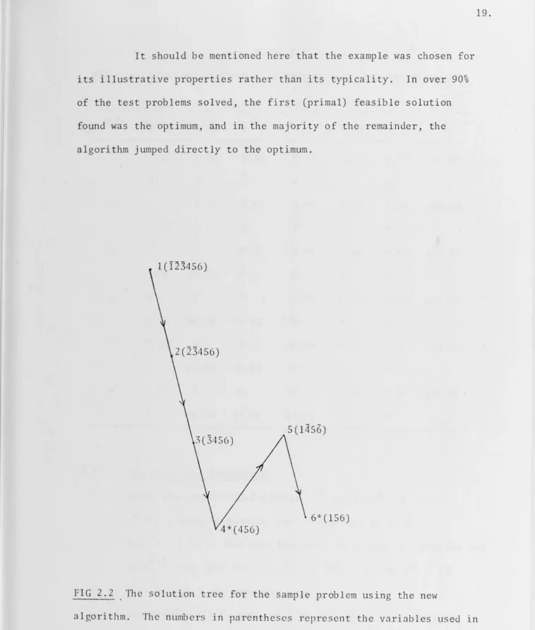
Figure 2.2 shows that portion of the tree generated using

Theorems 2.2 and 2.3 on the test problem of Fig. 2.1. The nodes

generated are given in Table 2.3. The first four nodes correspond to nodes 1 to 4 of the earlier tree, and nodes 5 and 6 correspond to nodes 9 and 10 respectively. In terms of the primal/dual feasibility

discussion of Section 2.1.1, nodes 1 and 2 are dual feasible, node 3 is

neither dual nor primal feasible, node 4 is primal feasible, node 5 is

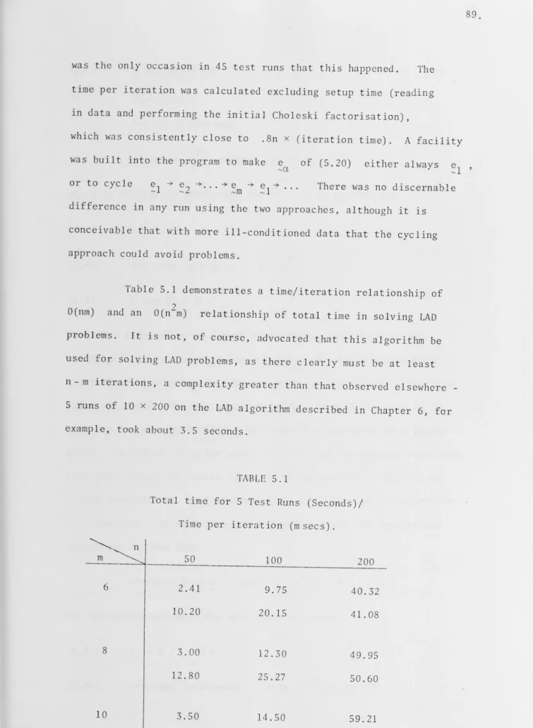
It should be mentioned here that the example was chosen for

its illustrative properties rather than its typicality. In over 90%

of the test problems solved, the first (primal) feasible solution

found was the optimum, and in the majority of the remainder, the

algorithm jumped directly to the optimum.

1(123456)

2(23456)

6*(156)

FIG 2.2 TI1e solution tree for the sample problem using the new

algorithm. The numbers in parentheses represent the variables used in

the solution, those with a-, being negative. An* indicates that

[image:27.780.6.764.21.913.2]

TABLE 2.3

Solutions obtained on the Sample Problem using the New Algorithm

2.2.5 Node

1

2

3

4

5

6

1.

2.

3.

xl/:\1 x2f;\2 X3/A3 X4/A4 X5/A5 x6/;\6 L(x)

-7.27 -1.89 -1. 34 0.92 2.91 1.70 32.09

0 0 0 0 0 0

0 -1.52 -1.05 0.44 2.23 1.08 36.42

1.19 0 0 0 0 0

0 0 -0.95 0.49 1.21 0.84 102.00

-3.12 86.03 0 0 0 0

0 0 0 0.25 0.84 0.62 127.18

-5.06 82.76 52.83 0 0 0

13.31 0 0 -0.53 0.22 -0.30 93.51

0 46.81 25.73 0 0 0

7.52 0 0 0 0.33 0.08 103.49

0 60.72 47.08 37.93 0 0

The Algorithm Summarised

Solve the unrestricted problem pl with Jl =

0

.

If

1 > _{0 stop; otherwise, set i +- 1 and go to 2.} X

-'

Set i +- i + 1

.

Use some heuristic to select k from the

{ I

_j i-1 }

X. < 0

J and 1 et J

1

= J 1 U { k } . Solve P1 . If

1

x ~ 0, go to 3; otherwise, go to 2.

Use Theorem 2.2 to test X l for optimality. If the test succeeds stop; otherwise, go to 4.

4. Use some heuristic to choose k from the set {j

I:\:<

O}

J

.

.

where :\1 = VL(x1) ; set i +- i + 1 , and let

-

-20.

set

J1

=

{

j

Ix~

-

1

=

o,

j

1

k} .

J Solve

[image:28.768.11.750.22.914.2]

otherwise, go to 5.

S. Set 1 + i + 1 . Choose k according to the method used 1n the proof of Lemma 2 .1. Let Ji ,= Ji-l U {k} _Solve

If _x l _{~ 0 , go to 3; otherwise, go to 5.}

The heuristics used in steps 2 and 4 were to choose the most negative variable in each case (but see Section 2.4 for a fuller

discussion) .

2. 3 COMPLEXITY

It appears difficult to determine any absolute complexity bounds for the algorithm, but if the assumption is made that, at any feasible _x r _{which fails the optimality test of 'lneorem 2.2, it does} so for only one variable, then linear bounds can be derived.

Theorem 2.4

If xr ~ 0 solves _{Pr ' 'r /\ = nL v (xr) , an d 'r /\. _ > 0}

l for

iEJr - {k} , then N , the number of subproblems solved, is at most 2n .

Proof Let

for all i EJr - {k} .

Then, by an argument similar to that used 1n proving Theorem 2.3,

Now Let

r+1 <

0

X.

l

for any X s ~ 0

J'

₌

{j Ix~ J

for all i EJr - {k} .

such that L (xs) < L (xr) _{assume that} s xk '

> 0 ' j E Jr}

.

0

Then there will exist a convex linear combination, yr~ 0 , of

r s

X , X and _X r+1 _{' l E J' '} which is feasible for and for

which L(yr) < L(xr) , which contradicts the optimality of X r

llence for each subsequent feasible solution, x s , foun<l after

r

X _'xk s > 0 _.

Now this applies at each step, so that after each feasible

solution is found by the algorithm, one more variable must remain

strictly positive. Thus, if Cl.

l ith feasible solution found, then

is the number held to zero in the

a. ~ n + 1 - 1 , and also there l

will be at most n feasible solutions found.

Let f. be the number of subproblems solved between the l

22.

(i - l)s~ (exclusive) and ith _(inclusive) feasible subproblems, . and F

the total number of feasible solutions found. Evidently, for 1 > 1 ,

f. = a. - a.

1 + 2, and if a0 is defined as 1, the formula is also

l l l

-correct for f 1 .

Thus

F

N =

l

f. i=l l

F

=

l

Cl. - _{Cl. 1} + 2

i=l l l

-~ 2F + n + 1 - F - 1

~ 2n .

Although there are no a priori grounds for supposing that

the above assumptions are always true, no case has yet been found in

with N = n , was the only instance of N/n ~ 1 (see Table 2.4).

2.4 RESULTS

The algorithm was tested against data generated using a

random number generator. For each problem size, ten sets of data were

solved. Due to lack of consistency of execution times, N, the

number of subproblems solved, was taken as the measure of algorithm

efficiency. (As an indication., however, solving problems with 40

variables and SO rows of data took 5 to 10 seconds on a Univac 1110/42.)

Armstrong and Frome claimed competitiveness for their algorithm, and as

it was the progenitor of the new algorithm, it was used for comparison

purposes. The results , given 1n Table 2.4, display the linearity

predicted 1n Section 2.3.

Of the several heuristics tested foi choosing the variable

to be set to zero at step 2 of the algorithm, choosing the most negative

and choosing the negative variable which had differed least from

proved best. The former was chosen for its simplicity. No choice

ever had to be made at step 4, but choosing the most negative

suggested.

2.5 EXTENSION TO OTHER PROBLEMS

A

.

1

1

X

lS

The features of the restricted least squares problem which

make it suitable for the algorithm as given are:

(i) the strict convexity of the objective function;

(ii) the special nature of the constraints; and

24.

Any problem which has the above properties 1s suitable for solving by the algorithm. One question which arises 1n other

applications is the optimality test if the Kuhn-Tucker conditions are not readily available, as this test 1s central to the algorithm. If this is the case, Theorem 2.2 can be replaced by one which requires solving no more than n - 1 additional subproblems to test the

optimality of a feasible solution to a subproblem.

Theorem 2.5

Let _X r > _- 0 _{solve pr Define Jr+1 = Jr - {i} for all}

E Jr _If r+i _{< 0 for al 1} E Jr, then r _{solves p}

1

.

n. 1 X

.

1

Proof

Assume the above conditions hold and further assume that there exists x' such that Now, for

x ! ~ 0

1 '

r+1 x.

1

and

< 0

r+1

X

so that

and for some ₁ . E Jr _' x! > 0 .

1 But, for

s

X

Hence there 1s a convex linear combination, for all i E Jr for which

' is feasible for

s

X. = 0

1 for all s

X

' of . E Jr

1 '

x'

Now L(x5) ~ convex linear combination (L(x'), L(xr+i)

for all i E Jr) . Since L(x') > L(xr) ,

contribution to

x'

of X s 1s non-zero, it follows that

Hence

which contradicts the assumption that r

x solves P .

r

X solves

Under the asswnptions of Theorem 2.4 (the complexity theorem),

it is easy to show that the number of subproblems solved is not more

than ~ (n + 1) . However, testing the modified algorithm on the same test data as used before indicated that in practice this algorithm also

behaves linearly (see Table 2.4).

2.6 CONCLUSION

The algorithm presented here appears to be a considerable

improvement on existing algorithms of branch and bound type for this

problem, without sacrificing any of the advantages of these algorithms,

for example, ease of use in an interactive mode, wide availability of

least squares regression routines, and simple modification to account

for variable bounds.

The reason would appear to be that in this problem, as so

often in branch and bound, the optimum solution is found quickly and

then much time is spent in the subsequent searching necessary to

verify it. Thus the biggest advantage of this approach is in the use

of optimality conditions to improve bounding. Incorporating this into

the general framework of branch and bound has resulted 1n a very

Dimension of A

n m

6 10

10 15

15 20

20 30

30 40

40 50

- TABLE 2. 4

Experimental results. Number of subproblems solved

Armstrong/Frame algorithm

Mean Worst

10.0 32

168.2 566

4097.8 11886

-

--

--

-Armstrong/Frame improved

Mean Worst

4.4 11

34.6 96

668.6 1947

-

--

-New Algorithm

Mean Worst

3.3 6

5.4 8

10.0 13

11.9 14·

16.6 19

24.4 28

New Algorithm modified

Mean Worst

4.9 13

8.8 14

18.0 24

21.8 26

31.2 36

46.8 54

N

CHAPTER

3

AN EFFICIENT IMPLEMENTATION OF THE LEAST

SQUARES ALGORITHM

3.1 INTRODUCTION

In the previous chapter we presented an algorithm for

solving the restricted least squares problem

(3.1)

minimise

subject to X ~ 0

In the original implementation of that algorithm, standard regression

routines were used to solve a new subproblem at each iteration. Now

although the algorithm appeared efficient in terms of the number of

subproblems solved (i.e. number of nodes of the search tree to be

visited), the implementation of the algorithm is still not good. In

this chapter we consider an improved implementation of the algorithm.

In particular, we want to provide methods which avoid solving each of

the unconstrained least squares problems ab initio when only one of

the variables is changed at each step. The key to our approach is

suggested by tl1e Kuhn-Tucker conditions which characterize the unique

minimum of

(3.1),

with uniqueness following from the strict convexity

of the objective function and the linearity of the constraints. These

conditions are

(3. 2a) - AT ( b - Ax) =

~

,

(3.2b)

(3.2c) A.X. =0,

l l

28.

1 = 1,2, ... ,n,

so that the subset selection problem can be restated as that of

seeking among all solutions satisfying the system of equations (3.2a) and the complementarity condition (3.2c) the unique pair satisfying

From our point of view the striking feature of this formulation is the symmetry between the roles of x an<l A • In particular it is possible to interchange the roles of _{and in} the algorithm. lbis has the advantage that a certain amount of

initial processing is avoided. For example, starting with x as the unconstrained minimizer of (3.1)~ is equivalent to rewriting (3.2a) in the form

( 3. 3)

and satisfying (3.2c) by setting A= 0

By the complementarity condition (3.2c), fixing a particular component of x at zero is equivalent to freeing the corresponding component of A • Thus we consider at each stage a partition of x ,

(3.4a) X =

[

~11

_~2

_J

with X = 0

~2 ~ '

and a corresponding partition of

A,

(3.4b)

~

₌

[t]

_with .\ = O ,

~l ~

whjch ensure c1utomatically that (3.2c) is satisfied. If (3.2a) is now solved for the variables permitted to be nonzero at the current stage then it can be written

where

(3

.

6)

_~A

_{= [}

~~]

_{and ~l}

_{= [;~]}

_·

Each step of the algorithm involves interchanging a component of x

with the corresponding component of A . This results in a .

transformation of (3 .5) which can be represented by multiplication

by an elementary Jordan matrix followed by appropriate permutations

to partition the new variables into the form

(3.6).

We define the

Jordan matrix J. by

l

(3.7)

J. K. (M) = ( I - j . e

! )

K. (M) = -e.

l l - l - l l - l '

where 1 is the index of the element of ~l to be exchanged, and

K

.

(

.

)

indicates that the ith column is taken. Using a bar to denote

l

transformed quantities we have

so

(3.8a)

and

(3.8b)

q = q _{q. J. '} l - l

q.M.k

- ' l l

q = q

-k k ~1-.

q.=

l

q.

l

-M ..

l l

l l

'

'

= (I-j.e!)Kk(M)

- l - l

k

f:

l '

k

f:

l

When k = i , the i th column of ~1 comes as a result of the interchange

A. -<-+ x. . This gives

l l

(3.8c) K. (~1) = -(I-j .e!)e.

l - l - l - l

=Ml ' {K. (M)+e.} - e. . . l - l - l

This shows that the computations involved in the algorithm can be

carried out in a manner familiar from stepwise regression (see eg,

Effroymsom, 1960). However, the problem set-up still involves the

calculation of the normal matrix which is a significant initial

computation.

30.

An alternative to forming the normal matrix is to apply

orthogonal transformations to the data matrix. This is known to have

superior numerical properties (see eg, Golub and Wilkinson, 1966)

but it is interesting that in the stepwise regression case it is

known to be more efficient for an important range of values of m

and n (Osborne, 1976). This approach is considered in the next

section. It turns out that set-up time can be considerably reduced

by working with the multiplier vector

A,

and there is an unexpected

bonus for ~₂ turns out to be a numerically better determined

quantity than ~l . Numerical results, including a comparison with

the quadratic programming approach, are presented in Section 3.3.

3.2 USE OF ORTHOGONAL TRANSFORMATIONS

To derive the equations satisfied by ~l and ~

2 we assume

that the orthogonal transformation of the data matrix is given by

(3.9) I\ =

Q

[O

u]

and

'

where

Q

is orthogonal and U upper triangular. Substituting 1n

(3.2a) gives

UTUx = _-UC T

or

(3.10) Ux =

We partition U and

:i

to conform with (3.4) by setting

(3 .11)

u

= and ~11

~12

so that (3 .10) reduces to the pair of equations

(3.12) and

1ne interchange of _{a pair A. '} X.

i l destroys the form of U unless the

last element of becomes the first element of

~2 or vice versa. Tilus the upper triangular form of U must be restored following an

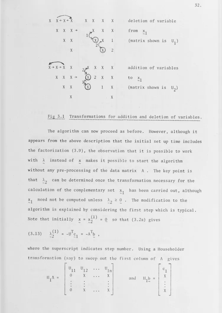
interchange, and this can be done using the now standard techniques treated 1n detail by Gill, et al, 1974. For example, to drop the kth element of

~l which we assume to be of length p > k , we perform the interchanges k + 1 + k, k + 2 + k + 1, . .. ,k + p on the columns of

u

1 and then sweep out the elements introduced ln the sub-diagonal positions using plane rotations W{j,j+l,(j+l,j)} , j = k,k + l, ... ,p - 1 where W{i,j,(p,q)} is the plane rotation mixing rows 1 and J and making

zero the element in the (p,q) position. Similarly, to add an element to

~l the corresponding column (say k) is moved to column 1

by the sequence of interchanges 1 + 2 · , 2 + 3, ... , k + 1 , and the upper triangular form is restored by the sequence of plane rotations

W{j,j+l,(j+l,l)} , j = k - 1, ... ,1 . 1nese operations are shown

32.

~

X X+-X+-X X X X X deletion of variable

X X X -+ X X X from

~l

1~,

X X 1 (matrix shown lS _Ul)

X 2

~ X-+X-+X X

2(_ X X X addition of variables

X X X -+

®

₂ X X to

~l

1~

X X

@

1 X (matrix shown lS _U2)

X X

Fig 3.1 Transformations for addition and deletion of variables.

The algorithm can now proceed as before. However, although it

appears from the above description that the initial set up time includes

the factorization (3.9), the observation that it is possible to work

with A instead of x makes it possible to start the algorithm

without any pre-processing of the data matrix A. The key point is

that _{~2 can} be determined once the transformation necessary for the calculation of the complementary set ~l has been carried out, although ~l need not be computed unless ~

2 ~ 0 . The modification to the algorithm is explained by considering the first step which 1s typical. Note that initially x

=

~il)

=

0 so that (3.2a) gives

(3.13) -UC T

---1

where the superscript indicates step number. Using a Householder

t.-r:i ns f o rm:1 ti on (sny) to S\vCCp out the First column of _I\ gives

u11 u12 uln cl

1

II/\ 0 X X anc.l _I1

1~

X

= ₌

[image:40.778.11.763.26.1082.2]

Now, from ( 3. 12) , we have

I

0 11

A ( 1)

0

12 cl

=

0(2)T (2)

-2 _:12

2 0

1n

0 11 0

12

0

= -c +

,

1 _A(2)

(3.14) 0

1n

-2

showing that the Lagrange multipliers can be updated and decisions

made on the order in which the remaining columns of A are swept

out as the factorization of A proceeds. Essentially no set-up

computations are required for this form of the algorithm.

This relation can be given a general form. We partition

Q so that (3.9) is written

(3.15)

Qrl

A

₌

[ul

and QTb

₌

~l

.

Q~

J

OJ

1~

Partitioning A and QT

1 1n conformity with X we obtain

(3.16) T _{[Ul Ul2 J} T _A2]

_[

_{o u}

2 J ,

Qll [Al A2]

=

and _Ql2[Al

=

34~

and, using (3.16),

-

[ ~2]

T T

= _{A Ql2Ql2~}

T T

( 3. 17) = _{A [I-QllQll]b}

'

as

and

In particular, the general form for (3.14) is

(3.18)

and this confirms that the multiplier vector is available when only

the transformation of A necessary to compute ~l has been completed.

Equation (3.18) is useful also as it permits an error analysis

for this method of computing ·\ to be given. Indicating computed

-2

quantities by bars we have

~2 - ~2

(3.19) _{= {u12} -T

where E is the evaluation error. This equation can be further

expanded to give

(3.20)

where the prime indicates the exact orthogonal factorization defined

by the actual numeric data at each stage. The quantities on the

The most important terms are those involving

Q

11 -

Q

11 , and it was

shown by Jennings and Osborne (1974) that this can be bounded by an

expression of the form k

1

eps

x(A

1

)

where k

1

is a constant, eps is

the machine precision, and

x(A

1

)

is the spectral condition number of

A

1 . This 1s a result which is more favourable than the corresponding

result for which Golub and Wilkinson (1966) showed to have a

dependence also on

~12

~2

However, the bounds quoted 1n the error estimate are for the usual

form of orthogonal factorization which takes. no account of the possibility of the back-tracking which can and does occur in the

algorithm. If we assume the analysis is valid also in the case of

back-tracking, then presumably we have to use the largest condition

number encountered to the present stage rather than the condition

number of the current partition A 1 .

One further point in favour of this form of the algorithm

is that it appears rarely to be necessary to compute the complete

factorization (3.9) in the determination of the optimum subset ~l

It is conceivable that the full system could be badly conditioned

while the subproblems leading to the optimal subset could be well

conditioned.

3.3 NUMERICAL RESULTS

A subset selection algorithm for (3.1) proceeds essentially in

two stages: an initial search for a feasible ~l (or ~

2) using a

heuristic to determine at each stage the component to be set to zero,

tree if the first feasible solution is not optimal. It is in this second phase of the computation that the major improvements due to

36.

the algorithm are achieved. In the first phase the heuristic commonly used is to fix at zero level the most negative of the current solution components. This procedure suffers from the disadvantage that it is not scale independent. For example, if the data matrix A 1s

multiplied by a diagonal matrix D to rescale the column norms so that

(3 .21a) A+- AD-l

'

then it follows from (3.2a) that the solution vectors are transformed by

(3.21b)

Our numerical experiments have shown that the choice of the first phase heuristic 1s important because it can affect the amount of work that has to be done 1n the second phase of the computation. It seems

reasonable that a good heuristic should not be affected by changes 1n scale, and for this reason we compare the choice of most negative

component with a choice which corresponds to the test used in stepwise regression to determine the variable to enter the regression at each step and which has the property of invariance with respect to column scaling. If we consider the data matrix factorized so that at the ith step of the first phase of the computation we have

( 3. 2 2) Ci)= [ 0

1 °12]

A O 13 and

then the stepwise regression test selects the variable to be introduced

I

dTK. (B)

I!

II

K. (B)

II '

- J J

as this leads to the biggest reduction in the sum of squares of the residuals (see Golub, 1965). Here

II

Kj (B)

II

is the euclidean length of the jth column of B . Now, from (3.18),

(3.23)

so that we can use the stepwise test in the form

(3.24) X +

-1 s maximizes

for all J such that y(j) > 0 .

y(j)

(~~i))j

IIK.(B)II

J

However, our implementation actually considers y(j) 2

II

K.(B)

11 2 is readily updated from step to step.

J

as

We report numerical results for two sets each of ten problems with m = 50

'

n = 40 . The data are obtained by sampling from a

normal distribution for the first set and from a uniform distribution for the second set, except that in all cases K

1 (A) j

=

1, j

=

1,2, ~ .. ,m.

For each set we give results for each of the selection strategies already discussed and for the case in which the most negative strategy is used after the columns of A are scaled initially to have unit length.

Also, for the data drawn from the uniform distribution, we consider scaling the columns of A to have unit

L

1

norm as the most negative strategy proved particuL1rly favourable in this case, and definitely superior to the corresponding scaling using the euclidean norm. Also, for comparison, we give results obtained using a quadratic programming subroutine QUADPR, based on the Cottle-Danzig principal pivoting

38.

The results for the two data sets are given 1n Tables 3.1

and 3.2 respectively. We report the average time per problem as

(cumulative time)/10 (recorded most unreliably on the computer used,

a Univac 1100/42)t, and the total number of nodes visited. It will

be seen that the variants of this algorithm are superior to the

quadratic programming algorithm. Also, the most negative heuristic

is never too bad, while the stepwise heuristic is favoured for the

data drawn from the normal distribution. · TI1crc is some evidence

that the statistical origin of the data is not irrelevant to the

choice of a good heuristic. Starting with A rather than x is

clearly the superior strategy in terms of elapsed time despite the

unreliability of the timings (for example, the stepwise and column

scaling strategies should have returned approximately the same times

in Tab 1 e 3 . 1) .

The rather dramatic 10-20 fold reduction in time taken

for this implementation seems to be partly due to the use of

orthogonalisation transformation techniques (as opposed to matrix

inversion in the original implementation), and partly due to working

with A rather than x - so that if, say, n/2 elements of x were

non-zero at the optimum, about\ of the elements of U in the QU

factorisation of A would need to be calculated, as opposed to 3/4

if working with x .

t Timings in a multiprogramming environment tend to be unreliable

because compromises are made between keeping exhaustive records and

efficiency. Part of the explanation in this case would appear to

stem from the system executive's practice of continuing the internal

timing of an interrupted program unless it is actually swapped out

TABLE 3.1

Results for data from normal distribution

Average time

Method _{(ms) Number of nodes}

Quadratic programming _{1187 404}

Most negative :\. 322 210

l

Stepwise _{249 204*}

II

Kj (A) 112 = 1 437 204*

Most negative X. _{547 202}

l

*First feasible solution is optimal for each problem.

TABLE 3.2

Results for data from uniform distribution

Average time

Method (ms) Number of nodes

Quadratic programming 1340 416

Most negative :\. 434 196

l

Stepwise 390 262

II

Kj (A) 112 385 262

IIKj(A)ll1

307 168

Most negative x. _l 518 240*

[image:47.776.9.760.16.1078.2]

4.1 4.1.1

CHAPTER 4

THEM-ESTIMATOR: STRUCTURE

INTRODUCTION

Robust Estimation and the Rejection of Outliers

The problem of rejection of outliers may not be quite as

old as experimental science, but it has certainly exercised the minds of astronomers, chemists, physicists, etc., for a very long time.

40.

The great German astronomer, Bessel, remarked in 1838 that he never rejected an observation merely because of its large residual. Others

have not been quite as confident of their equipment and procedures. The first attempt at a rejection criterion based on some sort of probability reasoning seems to have been given by Peirce in 1852. Since then, the topic has become a standard part of least squares

theory, and from 1925 onwards has received a great deal of attention from statisticians. An historical review is given by Anscombe (1960), where he also makes the pertinent observation that when a rejection

rule is applied, a judgement is not being made on the spuriousness or otherwise of the observation so much as protection is being sought against possible adverse effects - a rejection rule being something

akin to an insurance policy.

It is this safeguarding against small deviations from the assumptions that lies at the heart of the search for robust estimators, and any complacency in the use of classical estimators such as the

mean square deviation was shattered by Tukey in a rather entertaining article in 1960 with the aid of a simple example. He assumed a