High-order fluid solver based on a combined compact
integrated RBF approximation and its fluid structure
interaction applications
C.M.T. Tiena, D. Ngo-Conga, N. Mai-Duya, C.-D. Trana, T. Tran-Conga,∗
a
Computational Engineering and Science Research Centre, Faculty of Health, Engineering and Sciences, The University of Southern Queensland, Toowoomba,
Queensland 4350, Australia.
Abstract
In this study, we present a high-order numerical method based on a combined compact integrated RBF (IRBF) approximation for viscous flow and fluid structure interaction (FSI) problems. In the method, the fluid variables are locally approximated by using the combined compact IRBF, and the incom-pressible Navier-Stokes equations are solved by using the velocity-pressure formulation in a direct fully coupled approach. The fluid solver is verified through various problems including heat, Burgers, convection-diffusion equa-tions, Taylor-Green vortex and lid driven cavity flows. It is then applied to simulate some FSI problems in which an elastic structure is immersed in a viscous incompressible fluid. For FSI simulations, we employ the immersed boundary framework using a regular Eulerian computational grid for the fluid mechanics together with a Lagrangian representation of the immersed boundary. For the immersed fibre/membrane FSI problems, although the
or-∗
Corresponding author
der of accuracy of the present scheme is generally similar to FDM approaches reported in the literature, the present approach is nonetheless more accurate than FDM approaches at comparable grid spacings. The numerical results obtained by the present scheme are highly accurate or in good agreement with those reported in earlier studies of the same problems.
Keywords:
Combined compact integrated RBF; Convection-diffusion equations; Fluid flow; Fluid structure interaction; Enclosed membrane; Immersed boundary.
1. Introduction 1
Although many scientific and engineering problems involve fluid structure
2
interaction (FSI), thorough study of such problems remains a challenge due
3
to their strong nonlinearity and multidisciplinary requirements [1, 2, 3]. For
4
most FSI problems, closed form analytic methods to the model equations
5
are often not available, while laboratory experiments are not practical due to
6
limited resources. Therefore, to investigate the fundamental physics involved
7
in the complicated interaction between fluids and solids, one has to rely on
8
numerical methods [4].
9
In this study, we are interested in the interaction of a viscous
incom-10
pressible fluid with an immersed elastic membrane. The immersed
bound-11
ary method (IBM), originally developed by Peskin [5], is designed to solve
12
this kind of problem. The IBM is a mixed Eulerian-Lagrangian scheme in
13
which the fluid dynamics based on the Navier-Stokes (N-S) equations are
14
described in Eulerian form, and the elasticity of the structure is described in
15
Lagrangian form. The IBM considers the structure as an immersed boundary
which can be represented by a singular force in the N-S equations rather than
17
a real body. It avoids grid-conforming difficulties associated with the moving
18
boundary faced by conventional body-fitted methods. The fluid computation
19
is done on a fixed, uniform computational lattice and the representation of
20
the immersed boundary is independent of this lattice. The immersed
bound-21
ary exerts a singular force on the nearby lattice points of the fluid with the
22
help of a computational model of the Dirac δ-function. At the same time,
23
the representative material points of the immersed boundary move at the
lo-24
cal fluid velocity, which is obtained by interpolation from the nearby lattice
25
points of the fluid. The sameδ-function weights are used in the interpolation
26
step as in the application of the boundary forces on the fluid. Computer
sim-27
ulations using the IBM such as blood flow in the heart [5, 6], insect flight [7],
28
aquatic animal locomotion [8], bio-film processing [9], and flow past a pick-up
29
truck [10] have exhibited the great potential of the IBM in FSI applications.
30
Reviews on immersed methods can be found in [11, 12].
31
High-order approximation schemes have the ability to produce highly
ac-32
curate solutions to incompressible viscous flow problems. With these schemes,
33
a high level of accuracy can be achieved using a relatively coarse
discretisa-34
tion. Many types of high-order approximation methods have been reported
35
in the literature. Botella and Peyret [13] developed a Chebyshev
collo-36
cation method for the lid-driven cavity flow. Various types of high-order
37
compact finite difference algorithms (HOC) were proposed [14, 15, 16]. On
38
the other hand, radial basis function networks (RBF) have emerged as a
39
powerful approximation tool [17, 18, 19]. Different schemes of integrated
40
RBF approximation (here referred to as IRBF) were developed in the
erature [20, 21, 22, 23]. In [24], the authors developed a high-order fully
42
coupled scheme based on compact IRBF approximations for viscous flow
43
problems, where nodal first- and second-derivative values are included in
44
the stencil approximation and the starting points in the integration process
45
are second-order derivatives. In their work, the N-S governing equations
46
are taken in the primitive form where the velocity and pressure fields are
47
solved in a direct fully coupled approach. With relatively coarse meshes, the
48
compact IRBF produces very accurate solutions to many fluid flow
prob-49
lems in comparison with some other methods such as the standard central
50
finite different method (FDM) and HOC. Recently, Tien et al. [25] proposed
51
a combined compact IRBF approximation scheme, where nodal first- and
52
second-derivative values are also included in the stencil approximation, but
53
the starting points are fourth-order derivatives. The fourth-order IRBF
ap-54
proach allows a more straightforward incorporation of nodal values of
first-55
and second-order derivatives, and yields better accuracy over previous IRBF
56
approximation schemes.
57
In this paper, we will incorporate the high-order combined compact IRBF
58
approximation introduced in [25] into the fully coupled N-S approach
re-59
ported in [24]. The new high-order fluid solver is verified through various
60
problems such as heat, Burgers, convection-diffusion equations, Taylor-Green
61
vortex and lid driven cavity flows. It will show that highly accurate results
62
are obtained with the present approach. Then, we embed the fluid solver in
63
the IBM procedure outlined in [26, 27] to simulate FSI problems in which
64
a stretched elastic fibre/membrane relaxes in a viscous fluid. Comparisons
65
between the present scheme and some others, where appropriate, are
sented; and, numerical studies of the grid convergence and order of accuracy
67
are also included.
68
The remainder of this paper is organised as follows: Sections 2 first
re-69
views the spatial disretisation using the combined compact IRBF. Following
70
this, Section 3 briefly describes the fully coupled approach for N-S
equa-71
tions. Section 4 summarises the mathematical formulation of the IBM. In
72
Section 5, various numerical examples are presented and the present results
73
are compared with some benchmark solutions, where appropriate. Finally,
74
concluding remarks are given in Section 6.
75
2. Review of combined compact IRBF scheme 76
Consider a two-dimensional domain Ω, which is represented by a uniform
77
Cartesian grid. The nodes are indexed in the x-direction by the subscript
78
i (i ∈ {1,2, ..., nx}) and in the y-direction by j (j ∈ {1,2, ..., ny}). For
79
rectangular domains, let N be the total number of nodes (N = nx ×ny)
80
and Nip be the number of interior nodes (Nip= (nx−2)×(ny−2)). At
81
an interior grid point xi,j = (x(i,j), y(i,j))T where i ∈ {2,3, ..., nx − 1} and
82
j ∈ {2,3, ..., ny−1}, the associated stencils to be considered here are two local
83
stencils: {x(i−1,j), x(i,j), x(i+1,j)} in the x-direction and {y(i,j−1), y(i,j), y(i,j+1)}
84
in they-direction. Hereafter, for brevity,η denotes either xory in a generic
85
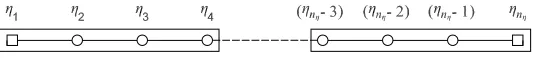
local stencil {η1, η2, η3}, where η1 < η2 < η3, as illustrated in Figure 1.
86
The integral process of the present combined compact IRBF starts with the decomposition of fourth-order derivatives of a variable, u, into RBFs
d4u(η)
dη4 =
m
X
i=1
wiGi(η). (1)
Approximate representations for the third- to first-order derivatives and the functions itself are then obtained through the integration processes
d3u(η)
dη3 =
m
X
i=1
wiI1i(η) +c1, (2)
d2u(η)
dη2 =
m
X
i=1
wiI2i(η) +c1η+c2, (3)
du(η)
dη =
m
X
i=1
wiI3i(η) + 1 2c1η
2+c
2η+c3, (4)
u(η) = m
X
i=1
wiI4i(η) + 1 6c1η
3+ 1 2c2η
2+c
3η+c4, (5) where I1i(η) =
R
Gi(η)dη; I2i(η) = R I1i(η)dη; I3i(η) = R I2i(η)dη; I4i(η) =
87
R
I3i(η)dη; and, c1, c2, c3, and c4 are the constants of integration. The
88
analytic form of the IRBFs up to eighth-order can be found in [28]. It is
89
noted that, for the solution of second-order PDEs, only (3-5) are needed.
90
2.1. First-order derivative approximations
91
For the combined compact approximation of the first-order derivatives at interior nodes, extra information is chosen as not only ndu1
dη ; du3
dη
o
but also
n
d2
u1
dη2 ;
d2
u3
dη2
o
follows. u1 u2 u3 du1 dη du3 dη d2 u1 dη2 d2 u3 dη2 = I4 I3 I2
| {z }
C w1 w2 w3 c1 c2 c3 c4 , (6)
where dui
dη = du
dη(ηi) with i∈ {1,2,3};Cis the conversion matrix; and, I2, I3, and I4 are defined as
I2 =
I21(η1) I22(η1) I23(η1) η1 1 0 0
I21(η3) I22(η3) I23(η3) η3 1 0 0
. (7)
I3 =
I31(η1) I32(η1) I33(η1)
1 2η
2
1 η1 1 0
I31(η3) I32(η3) I33(η3) 12η23 η3 1 0
. (8)
I4 =
I41(η1) I42(η1) I43(η1) 16η13 12η 2
1 η1 1
I41(η2) I42(η2) I43(η2) 16η23 12η 2
2 η2 1
I41(η3) I42(η3) I43(η3) 16η33 12η 2
3 η3 1
. (9)
Solving (6) yields
w1 w2 w3 c1 c2 c3 c4
which maps the vector of nodal values of the function and its first- and second-order derivatives to the vector of RBF coefficients including the four integration constants. The first-order derivative at the middle point is computed by substituting (10) into (4) and taking η=η2
du2
dη =I3mC
−1 | {z }
D1 u du1 dη du3 dη d2 u1 dη2 d2 u3 dη2 , (11) or du2
dη =D1(1 : 3)u+D1(4 : 5)
du1 dη du3 dη
+D1(6 : 7)
d2 u1 dη2 d2 u3 dη2
, (12)
where D1 is a row vector of length 7, the associated notation “a:b” is used to indicate the vector entries from the the column a to b; u = [u1, u2, u3]T; and,
I3m =
h
I31(η2) I32(η2) I33(η2) 12η22 η2 1 0
i
. (13)
By taking derivative terms to the left side and nodal variable values to the right side, (12) reduces to
h
−D1(4) 1 −D1(5)
i
u′
+h −D1(6) 0 −D1(7)
i
u′′
=D1(1 : 3)u,
(14) where u′
=hdu1
dη, du2 dη , du3 dη iT
and u′′
=hd2
u1
dη2 ,
d2
u2
dη2 ,
d2 u3 dη2 iT . 92
Figure 2: Special compact 4-point 1D-IRBF stencil for boundary nodes.
as du2
dη and d2
u2
dη2 . The conversion system over this special stencil is presented
as the following matrix-vector multiplication
u1 u2 u3 u4 du2 dη d2 u2 dη2 = I4sp I3sp I2sp
| {z }
Csp w1 w2 w3 w4 c1 c2 c3 c4 , (15)
where Csp is the conversion matrix; and, I2sp, I3sp, and I4sp are defined as
I2sp =h I21(η2) I22(η2) I23(η2) I24(η2) η2 1 0 0
i
. (16)
I3sp =
h
I31(η2) I32(η2) I33(η2) I34(η2) 12η22 η2 1 0
i
. (17)
I4sp =
I41(η1) I42(η1) I43(η1) I44(η1) 16η13 12η12 η1 1
I41(η2) I42(η2) I43(η2) I44(η2) 16η23 12η 2
2 η2 1
I41(η3) I42(η3) I43(η3) I44(η3) 16η33 12η32 η3 1
I41(η4) I42(η4) I43(η4) I44(η4) 16η43 12η 2
4 η4 1
Solving (15) yields w1 w2 w3 w4 c1 c2 c3 c4
=C−1
sp u1 u2 u3 u4 du2 dη d2 u2 dη2 . (19)
The boundary value of the first-order derivative of u is thus obtained by substituting (19) into (4) and taking η =η1
du1
dη =I3bC
−1
sp
| {z }
D1sp
u du2 dη d2 u2 dη2 , (20) or du1
dη =D1sp(1 : 4)u+D1sp(5) du2
dη +D1sp(6) d2u
2
dη2 , (21)
where u= [u1, u2, u3, u4]T and
I3b =
h
I31(η1) I32(η1) I33(η1) I34(η1) 12η21 η1 1 0
i
. (22)
By taking derivative terms to the left side and nodal variable values to the right side, (21) reduces to
h
1 −D1sp(5) 0 0
i
u′
+h 0 −D1sp(6) 0 0
i
u′′
=D1sp(1 : 4)u, (23)
where u′
=hdu1
dη, du2 dη , du3 dη, du4 dη iT
and u′′
=hd2u1
dη2 ,
d2
u2
dη2 ,
d2
u3
dη2 ,
2.2. Second-order derivative approximations
94
For the combined compact approximation of the second-order derivatives at interior nodes, we employ the same extra information used in the approx-imation of the first-order derivative, involving ndu1
dη ; du3
dη
o
and nd2u1
dη2 ;
d2
u3
dη2
o
. Therefore, the second-order derivative at the middle point is computed by simply substituting (10) into (3) and taking η =η2
d2u2
dη2 =I2mC
−1 | {z }
D2 u du1 dη du3 dη d2 u1 dη2 d2 u3 dη2 , (24) or
d2u 2
dη2 =D2(1 : 3)u+D2(4 : 5)
du1 dη du3 dη
+D2(6 : 7) d2 u1 dη2 d2 u3 dη2
, (25)
where u= [u1, u2, u3]T and
I2m =
h
I21(η2) I22(η2) I23(η2) η2 1 0 0
i
. (26)
By taking derivative terms to the left side and nodal variable values to the right side, (25) reduces to
h
−D2(4) 0 −D2(5)
i
u′
+h −D2(6) 1 −D2(7)
i
u′′
=D2(1 : 3)u,
(27) where u′
=hdu1
dη, du2 dη , du3 dη iT
and u′′
=hd2u1
dη2 ,
d2
u2
dη2 ,
d2 u3 dη2 iT . 95
At the boundary nodes, i.e. η = η1, we employ the same special sten-cil, i.e. {η1, η2, η3, η4}, and extra information, i.e. dudη2 and d
2
u2
approximation of the first-order derivatives. Therefore, approximate expres-sion for the second-order derivative atη1 in the physical space is obtained by simply substituting (19) into (3) and taking η =η1
d2u 1
dη2 =I2bC
−1
sp
| {z }
D2sp
u du2 dη d2 u2 dη2 , (28) or
d2u 1
dη2 =D2sp(1 : 4)u+D2sp(5)
du2
dη +D2sp(6) d2u
2
dη2 , (29)
where u= [u1, u2, u3, u4]T and
I2b =
h
I21(η1) I22(η1) I23(η1) I24(η1) η1 1 0 0
i
. (30)
By taking derivative terms to the left side and nodal variable values to the right side, (29) reduces to
h
0 −D2sp(5) 0 0
i
u′
+h 1 −D2sp(6) 0 0
i
u′′
=D2sp(1 : 4)u, (31)
where u′
=hdu1
dη, du2 dη , du3 dη, du4 dη iT
and u′′
=hd2u1
dη2 ,
d2
u2
dη2 ,
d2
u3
dη2 ,
d2 u4 dη2 iT . 96
2.3. Matrix assembly for first- and second-order derivative approximations
97
expressed as
A1 B1
A2 B2
| {z }
Coefficient matrix
u′n
u′′n
=
R1
R2
un , (32)
whereA1,A2,B1,B2,R1, andR2arenη×nη matrices;u′n =
h
u′
1 n
, u′
2 n
, ..., u′
nη
niT ;
u′′n
= hu′′
1 n
, u′′
2 n
, ..., u′′
nη
niT
; and, un = u1n, u2n, ..., unη
nT. The coefficient
matrix is sparse with diagonal sub-matrices. Solving (32) yields
u′n
=Dηun, (33)
u′′n
=Dηηun, (34)
where Dη and Dηη are nη ×nη matrices.
98
2.4. Numerical implementation
99
For convenience in terms of numerical implementation, the formulation
100
developed in Section 2.1 to 2.3 can be written in an intrinsic coordinate
101
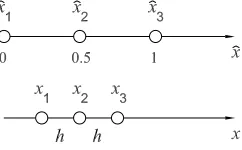
[image:13.595.244.365.488.563.2]system as shown in Figure 3 (top).
Figure 3: Intrinsic coordinate system (top), ˆx, and actual coordinate system (bottom),x, in whichhis actual grid size.
102
par-ticular grid size, h, Figure 3 (bottom), is as follows.
du
dx =
du dxˆ
dxˆ
dx =
1 2h
du
dxˆ. (35)
d2u
dx2 = 1 (2h)2
d2u
dxˆ2. (36)
Thus, the conversion matrix, C, needs be computed and inverted once.
103
Subsequently, as the grid size h changes, these matrices can be obtained by
104
a simple factor.
105
The present compact IRBF stencils can be extended to the three-dimensional
106
case since their approximations in each direction are constructed
indepen-107
dently. As shown above, the IRBF approximation expressions are first
de-108
rived in 1D and they are utilised to form the approximations in 2D. This
109
procedure is also applicable to the 3D case.
110
3. Review of fully coupled procedure for Navier-Stokes 111
The transient N-S equations for an incompressible viscous fluid in the primitive variables are expressed in the dimensionless non-conservative forms as follows.
∂u
∂t +
u∂u ∂x +v
∂u ∂y
| {z }
N(u)
=−∂p
∂x +
1
Re
∂2u
∂x2 +
∂2u
∂y2
| {z }
L(u)
, (37)
∂v
∂t +
u∂v ∂x+v
∂v ∂y
| {z }
N(v)
=−∂p
∂y +
1
Re
∂2v
∂x2 +
∂2v
∂y2
| {z }
L(v)
, (38)
∂u
∂x +
∂v
whereu,vandpare the velocity components in thex-,y-directions and static
112
pressure, respectively; Re=Ul/ν is the Reynolds number, in which ν, l and
113
U are the kinematic viscosity, characteristic length and characteristic speed
114
of the flow, respectively. For simplicity, we employ notationsN(u) andN(v)
115
to represent the convective terms in the x- and y-directions, respectively;
116
and, L(u) and L(v) to denote the diffusive terms in the x- and y-directions,
117
respectively.
118
The temporal discretisations of (37)-(39), using the Adams-Bashforth scheme for the convective terms and Crank-Nicolson scheme for the diffu-sive terms, result in
un−un−1
∆t +
3 2N(u
n−1
)−1 2N(u
n−2
)
=−Gx(pn−1
2)+ 1
2Re
L(un) +L(un−1
) ,
(40)
vn−vn−1
∆t +
3 2N(v
n−1
)− 1 2N(v
n−2
)
=−Gy(pn−1
2)+ 1
2Re
L(vn) +L(vn−1
) ,
(41)
Dx(un) +Dy(vn) = 0, (42)
where n denotes the current time level; Gx and Gy are gradients in the x
-119
and y-directions, respectively; and, Dx and Dy are gradients in the x- and
120
y-directions, respectively.
121
Taking the unknown quantities in (40)-(42) to the left hand side and the known quantities to the right hand side, and then collocating them at the interior nodal points result in the matrix-vector form
K 0 Gx
0 K Gy
Dx Dy 0
un vn
pn−1
2 =
rnx
rny
where
K= 1
∆t
I− ∆t
2ReL
, (44)
rnx = 1 ∆t
I+ ∆t
2ReL
un−1
−
3 2N(u
n−1
)− 1 2N(u
n−2
)
, (45)
rny = 1 ∆t
I+ ∆t
2ReL
vn−1
−
3 2N(v
n−1
)− 1 2N(v
n−2
)
, (46)
un andvnare vectors containing the nodal values ofunand vnat the
bound-122
ary and interior nodes, respectively, while pn−1
2 is a vector containing the 123
values of pn−1
2 at the interior nodes only; I is the identity matrix; and, N 124
and L are the matrix operators for the approximation of the convective and
125
diffusive terms, respectively.
126
4. Summary of immersed boundary method 127
In this section, we provide a brief overview of the IBM and the reader is
128
referred to [26, 27] for further details. For simplicity, we consider a model
129
problem of a two-dimensional Newtonian, incompressible fluid and a
one-130
dimensional, closed, elastic membrane. The fluid is defined on a periodic box
131
Ω = [0,1]2 using the Eulerian coordinates x= (x, y). The fluid contains an
132
immersed neutrally-buoyant membrane Γ⊂Ω, using the Lagrangian
coordi-133
natess ∈[0,1]. It is noted that the lattice points are fixed but the boundary
134
points are moving, and those two sets of points usually do not coincide with
135
each other. We discretise Ω using a uniform nx×ny grid. Then, we set the
136
mesh size of the immersed boundary to be nb = 3×nx, so that there are
137
approximately 3 immersed boundary points per mesh width.
138
fluid-membrane is governed by the incompressible N-S equations
ρ
∂u
∂t +u· ∇u
=−∇p+µ∇2u+f, (47)
∇ ·u= 0, (48)
where u = u(x, t) = (u(x, t), v(x, t)) and p = p(x, t) are the fluid velocity and pressure at location x and time t, respectively; ρ and µ are the con-stant fluid density and dynamic viscosity, respectively; and, f = f(x, t) = (fx(x, t), fy(x, t)) is the external body force through which the immersed boundary is coupled to the fluid
f(x, t) =
Z
Γ
F(s, t)δ(x−X(s, t))ds, (49)
where X(s, t) = (X(s, t), Y(s, t)) is a parametric curve representing the im-mersed boundary configuration; the delta function δ(x) = dh(x)dh(y) is a Cartesian product of one-dimensional Dirac delta functions, which is used to spread the Lagrangian immersed boundary force from Γ onto adjacent Eulerian fluid nodes. The one-dimensional Dirac delta function is chosen as
dh(r) =
1 8h
3−2|r|/h+
q
1 + 4|r|/h−4 (|r|/h)2
, |r| ≤h,
1 8h
5−2|r|/h−
q
−7 + 12|r|/h−4 (|r|/h)2
, h≤ |r| ≤2h,
0, otherwise,
(50) in which h is the grid size; and, F(s, t) is the elastic force density which is a function of the current immersed boundary configuration
F(s, t) =F(X(s, t)) = σ ∂
∂s
∂X(s, t)
∂s 1−
ε
|∂X∂s(s,t)|
!!
which corresponds to membrane points linked together by linear springs with spring constant σ. If we assume the equilibrium strain ε = 0, then (51) reduces to
F(s, t) =F(X(s, t)) =σ∂
2X(s, t)
∂s2 . (52)
The final equation needed to close the system is an evolution equation for the immersed boundary, which comes from the simple requirement that Γ must travel at the local fluid velocity (the non-slip condition)
∂X(s, t)
∂t =U(X(s, t), t) =
Z
Ω
u(x, t)δ(x−X(s, t))dx, (53)
where U is the boundary speed. The delta function δ here imposes the
139
Eulerian flow velocity on the adjacent Lagrangian boundary nodes.
140
IBM algorithm. Next, we describe the algorithm used in this work, which is
141
a discrete version of Equations (47), (48), (49), (51), and (53). Assuming
142
that the velocity field and the membrane position are already known at time
143
tn−2
, tn−3/2
, andtn−1
. The procedure for updating these values to time tn is
144
as follows.
145
At half time step:
146
Step 1. Update position of membrane
Xn−1/2
(s)−Xn−1
(s)
∆t/2 =
X
Ω
un−1
δ(x−Xn−1
(s))h2. (54)
Step 2. Compute membrane force density
Fn−1/2
(s) =F
Xn−1/2
(s). (55)
Step 3. Calculate force coming from membrane
fn−1/2
(x) = X Γ
Fn−1/2
(s)δ(x−Xn−1/2
Step 4. Solve for fluid motion
ρ
un−1/2
−un−1
∆t/2 +
3 2N u
n−1
− 12N un−2
=Gp˜n−1/2
+µ 2
L un−1/2
+L un−1
+fn−1/2
. (57)
D·un−1/2
= 0. (58)
Once un−1/2
are known, we use them to take a full step from time tn−1
totn,
147
as follows.
148
At full time step:
149
Step 5. Solve for fluid motion
ρ
un−un−1
∆t +
3 2N u
n−1/2
− 12N un−3/2
=Gpn−1/2
+µ 2
L(un) +L un−1
+fn−1/2
. (59)
D·un= 0. (60)
Step 6. Update position of membrane
Xn(s)−Xn−1
(s)
∆t =
X
Ω
un−1/2
δ(x−Xn−1/2
(s))h2. (61)
5. Numerical examples 150
We chose the multiquadric (MQ) function as the basis function in the present calculations
Gi(x) =
q
(x−ci)2+a2i, (62)
where ci and ai are the centre and the width of the i-th MQ, respectively.
151
For each stencil, the set of nodal points is taken to be the same as the set
of MQ centres. We simply choose the MQ width as ai =βhi, where β is a
153
positive scalar and hi is the distance between the i-th node and its closest
154
neighbour. The value ofβ = 10 is chosen for calculations in the present work.
155
We evaluate the performance of the present scheme through the following
156
measures
157
i. The root mean square error (RMS) is defined as
RMS =
s PN
i=1 fi−fi
2
N , (63)
where fi and fi are the computed and exact values of the solution f
158
at the i-th node, respectively; and, N is the number of nodes over the
159
whole domain.
160
ii. The maximum absolute error (L∞) is defined as
L∞= max
i=1,...,N|fi−fi|. (64) iii. The global convergence rate, α, with respect to the grid refinement is
defined through
RMS(h)≈γhα =O(hα), (65)
where h is the grid size; and, γ and α are exponential model’s
param-161
eters.
162
iv. A flow is considered as reaching its steady state when
s PN
i=1 fin−fn
−1
i
2
N <10
−9
. (66)
v. Difference (%) between computed and analytical values is defined to be
f −f
For comparison purposes, we also implement the standard FDM, HOC
163
scheme of Tian et al. [15] and coupled compact IRBF scheme of Tien et al.
164
[23] for numerical calculations.
165
5.1. Heat equation
166
By selecting the following heat equation, the performance of the present combined compact IRBF scheme can be studied for the diffusive term only as
∂u
∂t =
∂2u
∂x2, a≤x≤b, t≥0, (68)
u(x,0) =u0(x), a≤x≤b, (69)
u(a, t) =uΓ1(t) and u(b, t) = uΓ2(t), t≥0, (70)
whereuandtare the field variable and time, respectively; and,u0(x),uΓ1(t),
and uΓ2(t) are prescribed functions. The temporal discretisation of (68) with
the Crank-Nicolson scheme gives
un−un−1
∆t =
1 2
∂2un
∂x2 +
∂2un−1
∂x2
, (71)
where the superscript n denotes the current time step. (71) can be rewritten as
1− ∆t 2
∂2
∂x2
un=
1 + ∆t 2
∂2
∂x2
un−1
. (72)
Consider (68) on a segment [0, π] with the initial and boundary conditions
u(x,0) = sin(2x), 0< x < π. (73)
u(0, t) = u(π, t) = 0, t≥0. (74)
The exact solution of this problem can be verified to be
u(x, t) = sin(2x)e−4t
The spatial accuracy of the present scheme is investigated using various
uni-167
form grids {11,13, ...,25}. We employ here a small time step, ∆t = 10−6
,
168
to minimise the effect of the approximation error in time. The solution is
169
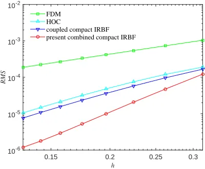
computed at t= 0.0125. Figure 4 shows that the present combined compact
170
IRBF outperforms the standard central FDM, HOC, coupled compact IRBF
171
in terms of both the solution accuracy and convergence rate.
h
0.15 0.2 0.25 0.3
RMS
10-6 10-5 10-4 10-3 10-2
FDM HOC
[image:22.595.197.397.271.436.2]coupled compact IRBF present combined compact IRBF
Figure 4: Heat equation, {11,13, ...,25}, ∆t = 10−6
, t = 0.0125: The effect of the grid size hon the solution accuracyRM S. The solution converges asO(h1.96) for the central
FDM, O(h3.34) for the HOC, O(h3.54) for the coupled compact IRBF, and O(h5.35) for
the present combined compact IRBF.
172
5.2. Burgers equation
173
With Burgers equation, the performance of the present combined compact IRBF scheme can be investigated for both the convective and diffusive terms as
∂u
∂t +u
∂u
∂x =
1
Re ∂2u
u(x,0) =u0(x), a≤x≤b, (77)
u(a, t) =uΓ1(t) and u(b, t) = uΓ2(t), t≥0, (78)
where Re > 0 is the Reynolds number; and, u0(x), uΓ1(t), and uΓ2(t) are
prescribed functions. The temporal discretisations of (76) using the Adams-Bashforth scheme for the convective term and Crank-Nicolson scheme for the diffusive term, result in
un−un−1
∆t +
(
3 2
u∂u ∂x
n−1
− 1 2
u∂u ∂x
n−2)
= 1
2Re
∂2un
∂x2 +
∂2un−1
∂x2
,
(79) or
1− ∆t 2Re
∂2
∂x2
un=
1 + ∆t 2Re
∂2
∂x2
un−1
−∆t
(
3 2
u∂u ∂x
n−1
− 12
u∂u ∂x
n−2)
.
(80) The problem is considered on a segment 0≤x≤1 in the form [29]
u(x, t) = α0+µ0+ (µ0−α0) exp(λ)
1 + exp(λ) , (81)
where λ = α0Re(x−µ0t−β0), α0 = 0.4, β0 = 0.125, µ0 = 0.6, and Re =
174
200. The initial and boundary conditions can be derived from the analytic
175
solution (81). The calculations are carried out on a set of uniform grids
176
{61,71, ...,121}. The time step ∆t = 10−6
is chosen. The errors of the
177
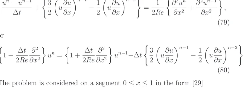
solution are calculated at the time t = 0.0125. Figure 5 shows that the
178
present combined compact IRBF overwhelms the standard central FDM,
179
HOC, coupled compact IRBF schemes in terms of both the solution accuracy
180
and convergence rate.
[image:23.595.115.523.279.432.2]h
0.01 0.012 0.014 0.016 0.018 0.02
RMS
10-5 10-4 10-3
FDM HOC
[image:24.595.197.396.135.295.2]coupled compact IRBF present combined compact IRBF
Figure 5: Burgers equation,{61,71, ...,121},Re= 200, ∆t= 10−6
,t= 0.0125: The effect of the grid sizehon the solution accuracyRM S. The solution converges asO(h1.96) for
the central FDM, O(h4.62) for the HOC, O(h5.03) for the coupled compact IRBF, and O(h5.81) for the present combined compact IRBF.
5.3. Convection-diffusion equations
182
To study the performance of the present combined compact IRBF ap-proximation in simulating convection-diffusion problems, we employ the al-ternating direction implicit (ADI) procedure which was detailed in [23]. A two-dimensional unsteady convection-diffusion equation for a variable u is expressed as follows.
∂u ∂t +cx
∂u ∂x +cy
∂u ∂y =dx
∂2u
∂x2 +dy
∂2u
∂y2 +fb, (x, y, t)∈Ω×[0, T], (82) subject to the initial condition
u(x, y,0) =u0(x, y), (x, y)∈Ω, (83)
and the Dirichlet boundary condition
where Ω is a two-dimensional rectangular domain; Γ is the boundary of Ω;
183
[0, T] is the time interval; fb is the driving function; u0 and uΓ are some
184
given functions; cx and cy are the convective velocities; and, dx and dy are
185
the diffusive coefficients.
186
In this work, we considerfb = 0, in a square Ω = [0,2]2 with the following analytic solution [30]
u(x, y, t) = 1 4t+ 1exp
−(x−cxt−0.5) 2
dx(4t+ 1) −
(y−cyt−0.5)2
dy(4t+ 1)
, (85)
and subject to the Dirichlet boundary condition. From (85), one can derive
187
the initial and boundary conditions. We consider two sets of parameters
188
Case I: cx =cy = 0.8, dx =dy = 0.01, t = 0.0125, ∆t = 1E−6.
189
Case II:cx =cy = 80, dx=dy = 0.01, t = 0.0125, ∆t = 1E−6.
190
The corresponding Peclet number is thusP e= 2 for case I andP e= 200
191
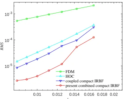
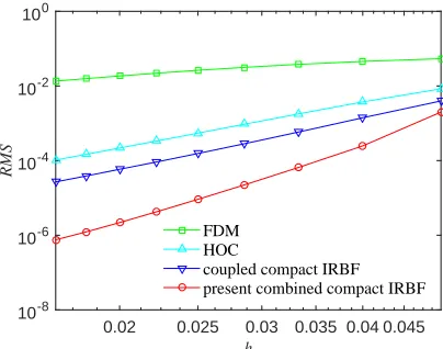
for case II. Figures 6 and 7 show analyses of the solution accuracy when the
192
grid size is refined. It can be seen that the accuracy and convergence rate of
193
the present combined compact IRBF scheme are much better than those of
194
the central FDM, HOC, and coupled compact IRBF.
195
5.4. Taylor-Green vortex
196
To study the performance of the combination of the combined compact IRBF and the fully coupled approaches in simulating viscous flow, we con-sider a transient flow problem, namely Taylor-Green vortex [15]. This prob-lem is governed by the N-S equations (40)-(42) and has the analytical solu-tions
u(x1, x2, t) =−cos(kx1) sin(kx2) exp(−2k2t/Re), (86)
h
0.02 0.03 0.04 0.05 0.06
RMS
10-10 10-8 10-6 10-4 10-2
FDM HOC
[image:26.595.191.398.135.297.2]coupled compact IRBF present combined compact IRBF
Figure 6: Unsteady convection-diffusion equation, {31×31,41×41, ...,121×121}, case I: The effect of the grid size hon the solution accuracyRM S. The solution converges as
O(h1.90) for the central FDM, O(h4.29) for the HOC, O(h4.71) for the coupled compact
IRBF, andO(h7.02) for the present combined compact IRBF.
h
0.02 0.025 0.03 0.035 0.04 0.045
RMS
10-8 10-6 10-4 10-2 100
FDM HOC
coupled compact IRBF present combined compact IRBF
Figure 7: Unsteady convection-diffusion equation, {41×41,51×51, ...,121×121}, case II: The effect of the grid size h on the solution accuracyRM S. The solution converges asO(h1.28) for the central FDM,O(h4.04) for the HOC,O(h4.56) for the coupled compact
[image:26.595.194.396.416.575.2]p(x1, x2, t) =−1/4{cos(2kx1) + cos(2kx2)}exp(−4k2t/Re), (88)
where 0 ≤ x1, x2 ≤ 2π. Calculations are carried out for k = 2 on a set of
197
uniform grids, {11×11,21×21, ...,51×51}. A fixed time step ∆t = 0.002
198
and Re = 100 are employed. Numerical solutions are computed at t = 2.
199
The exact solutions, i.e. equations (86)-(88), provide the initial field att = 0
200
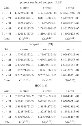
and the time-dependent boundary conditions. Table 1 shows the accuracy
201
comparison of the present scheme with the HOC scheme of Tian et al. [15]
202
and the compact IRBF scheme of Tien el al. [24]. It is seen that the present
203
scheme produces much better accuracy than the two other schemes; and,
204
its convergence rates are much higher than those of the HOC and compact
205
IRBF, i.e. O(h7.02) compared to O(h5.35) of the compact IRBF andO(h2.92)
206
of the HOC for the u-velocity; and, O(h8.51) compared to O(h4.48) of the
207
compact IRBF and O(h3.28) of the HOC for the pressure.
208
5.5. Lid driven cavity
209
The classical lid driven cavity flow has been considered as a test problem
210
for the evaluation of numerical methods and the validation of fluid flow solvers
211
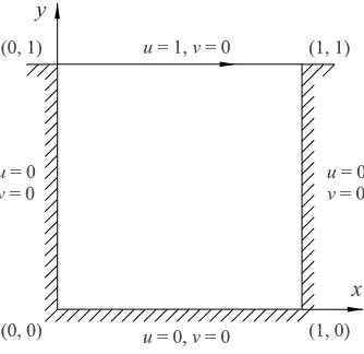
for the past decades. Figure 8 shows the problem definition and boundary
212
conditions. Uniform grids of {31×31,51×51,71×71,91×91,111×111}
213
and Re= 1000 are employed in the simulation. A fixed time step is chosen
214
to be ∆t = 0.001. Numerical results of the present scheme are compared
215
with those of some others [13, 24, 31, 32, 33, 34, 35, 36]. From the literature,
216
FDM results using very dense grids presented by Ghia et al. [31] and
pseudo-217
spectral results presented by Botella and Peyret [13] have been referred to as
218
“Benchmark” results for comparison purposes.
Table 1: Taylor-Green vortex: RM S-errors and convergence rates. present combined compact IRBF
Grid u-error v-error p-error 11×11 1.0652655E+00 1.0584558E+00 6.6053162E+00 21×21 6.4466038E-04 6.3416436E-04 5.5476571E-03 31×31 1.1927530E-04 1.1745523E-04 1.6486893E-04 41×41 1.8243332E-05 1.7849839E-05 1.8919708E-05 51×51 1.4261494E-05 1.2104415E-05 1.1300027E-05
Rate O(h7.02) O(h7.10) O(h8.51)
compact IRBF [24]
Grid u-error v-error p-error 11×11 1.7797233E-01 1.7797723E-01 3.0668704E-01 21×21 4.6366355E-03 4.6366340E-03 8.5913505E-03 31×31 5.3168859E-04 5.3168061E-04 2.6550518E-03 41×41 1.0970214E-04 1.0968156E-04 3.4713723E-04 51×51 3.2428099E-05 3.2378594E-05 2.6244035E-04
Rate O(h5.35) O(h5.35) O(h4.48)
HOC [15]
Grid u-error v-error p-error 11×11 7.0070489E-02 7.0070489E-02 1.0764149E-01 21×21 9.0692193E-03 9.0692193E-03 1.0567607E-02 31×31 2.8851487E-03 2.8851487E-03 2.9103288E-03 41×41 1.2238736E-03 1.2238736E-03 1.1356134E-03 51×51 6.3063026E-04 6.3063026E-04 5.3933641E-04
Figure 8: Lid driven cavity: problem configurations and boundary conditions.
Table 2 shows the present results for the extrema of the vertical and
220
horizontal velocity profiles along the horizontal and vertical centrelines of
221
the cavity. The “Errors” evaluated are relative to “Benchmark” results of
222
[13]. With relatively coarser grids, the results obtained by the present scheme
223
are very comparable with others using denser grids.
224
Figure 9 displays velocity profiles along the vertical and horizontal
cen-225
trelines for different grid sizes, where the grid convergence of the present
226
scheme is clearly observed (i.e. the present solution approaches the
bench-227
mark solution with a fast rate as the grid density is increased). The present
228
scheme effectively achieves the benchmark results with a grid of only 71×71
229
in comparison with the grid of 129×129 used to obtain the benchmark
re-230
sults in [31]. In addition, those velocity profiles, with the grid of 71×71,
231
are displayed in Figure 10, where the present solutions match the benchmark
232
ones very well.
233
To exhibit contour plots of the flow, Figures 11 and 12 show streamlines
Table 2: Lid driven cavity,Re= 1000: Extrema of the vertical and horizontal velocity profiles along the horizontal and vertical
centrelines of the cavity, respectively. “Errors” are relative to the “Benchmark” data.
Method Grid umin Error ymin vmax Error xmax vmin Error xmin
(%) (%) (%)
present combined compact IRBF 31×31 -0.3666974 5.63 0.1979 0.3550856 5.80 0.1601 -0.4851327 7.96 0.8932
present combined compact IRBF 51×51 -0.3756440 3.33 0.1760 0.3640018 3.43 0.1603 -0.5110586 3.04 0.9035
present combined compact IRBF 71×71 -0.3837160 1.25 0.1725 0.3717639 1.37 0.1590 -0.5210042 1.15 0.9078
present combined compact IRBF 91×91 -0.3866230 0.50 0.1718 0.3747332 0.59 0.1584 -0.5248188 0.43 0.9088
present combined compact IRBF 111×111 -0.3877643 0.21 0.1716 0.3759610 0.26 0.1581 -0.5262950 0.15 0.9091
compact IRBF (u, v,p), [24] 51×51 -0.3611357 7.06 0.1819 0.3481667 7.63 0.1621 -0.4853383 7.92 0.9025
compact IRBF (u, v,p), [24] 71×71 -0.3807425 2.01 0.1741 0.3685353 2.23 0.1593 -0.5156774 2.16 0.9079
compact IRBF (u, v,p), [24] 91×91 -0.3857664 0.72 0.1725 0.3738367 0.82 0.1585 -0.5231499 0.75 0.9089
compact IRBF (u, v,p), [24] 111×111 -0.3873278 0.32 0.1720 0.3755235 0.38 0.1582 -0.5254043 0.32 0.9091
compact IRBF (u, v,p), [36] 71×71 -0.3755225 3.36 0.1753 0.3637009 3.51 0.1608 -0.5086961 3.49 0.9078
compact IRBF (u, v,p), [36] 91×91 -0.3815923 1.80 0.1735 0.3698053 1.89 0.1594 -0.5174658 1.82 0.9085
compact IRBF (u, v,p), [36] 111×111 -0.3840354 1.17 0.1728 0.3722634 1.24 0.1588 -0.5209683 1.16 0.9088
compact IRBF (u, v,p), [36] 129×129 -0.3848064 0.97 0.1724 0.3729119 1.07 0.1586 -0.5223350 0.90 0.9089
FVM (u,v, p), [34] 128×128 -0.38511 0.89 — 0.37369 0.86 — -0.5228 0.81 —
FDM (ψ−ω), [31] 129×129 -0.38289 1.46 0.1719 0.37095 1.59 0.1563 -0.5155 2.20 0.9063
FEM (u,v, p), [32] 129×129 -0.375 3.49 0.160 0.362 3.96 0.160 -0.516 2.10 0.906
FDM (u,v,p), [33] 256×256 -0.3764 3.13 0.1602 0.3665 2.77 0.1523 -0.5208 1.19 0.9102
FVM (u,v, p), [35] 257×257 -0.388103 0.12 0.1727 0.376910 0.01 0.1573 -0.528447 0.26 0.9087
u
-0.5 0 0.5 1
y
0 0.2 0.4 0.6 0.8 1
present 31x31 present 51x51 present 71x71 present 91x91 Ghia et al. [28] 129x129
x
0 0.2 0.4 0.6 0.8 1
v
-0.6 -0.4 -0.2 0 0.2 0.4
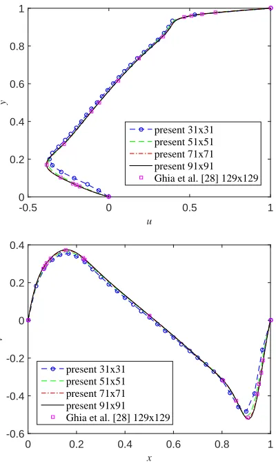
[image:31.595.201.401.198.535.2]present 31x31 present 51x51 present 71x71 present 91x91 Ghia et al. [28] 129x129
x
0 0.2 0.4 0.6 0.8 1
v
-1 -0.5 0 0.5 1
u
-1 -0.5 0 0.5 1
y
0 0.2 0.4 0.6 0.8 1
present 71x71
[image:32.595.205.414.123.288.2]Ghia et al. [28] 129x129
Figure 10: Lid driven cavity, Re = 1000: Profiles of the u-velocity along the vertical centreline and the v-velocity along the horizontal centreline.
and iso-vorticity lines, respectively, which are derived from the velocity field.
235
Figure 13 shows the pressure deviation contours of the present simulation.
236
These plots are also in good agreement with those reported in the literature.
[image:32.595.239.379.461.605.2]237
Figure 12: Lid driven cavity, Re = 1000, 91×91: Iso-vorticity lines of the flow. The contour values used here are taken to be the same as those in [31].
Figure 13: Lid driven cavity, Re = 1000, 91×91: Static pressure contours of the flow. The contour values used here are taken to be the same as those in [13].
238
5.6. Elastic flat fibre (surface)
239
[image:33.595.239.380.377.523.2]comparison purposes, we set up the problem parameters and configurations to be the same as those used in [37]. Figure 14 depicts the problem configu-rations. The fluid domain is a unit square with periodic boundary conditions
Figure 14: Fibre: The initial fibre position is a sinusoidal curve. The equilibrium state is a flat surface.
in the x- and y-directions. The viscosity and density constants are chosen as µ = 1 and ρ = 1, respectively. The initial position is a sinusoidal curve described by
X(s,0) =
s,1
2 +A sin(2πs)
, (89)
where the constant A is set to 0.05. The fluid is initially at rest
u(x,0) = 0. (90)
The purpose of this simulation is to test the decay rate of the maximum
240
height of the fibre. Figure 15 plots a sample of the computed maximum
241
height of the immersed fibre as a function of time, which oscillates with a
242
decaying amplitude. There are two quantities that can easily be obtained
243
from this information in order to make comparisons with the analytic results
244
[37]:
Figure 15: Fibre: A sample of computed maximum fibre height versus time.
i. The decay rate, Dr(λ), for the smallest wave number 2π mode which can be determined by measuring the rate at which the maximum fibre height decays to zero
Dr(λ) = 1
t2−t1
ln
H2
H1
. (91)
ii. The frequency, F r(λ), which can be calculated from the period of the fibre oscillations
F r(λ) = π
t2−t1
. (92)
The results are summarised in Table 3 for various values of the fibre spring
246
constant σ ={1,20,100,1000,10000,100000}. With relatively coarse grids,
247
the present decay rate shows very good agreement with the analytical results,
248
and so does the frequency. The relative difference is within 6.3% for all values
249
of σ. The decay rates produced by the present scheme are generally more
Table 3: Fibre: Analytical and computed values of the decay rateDr(λ) and frequencyF r(λ) for the solution mode with the
smallest wave number 2π. The difference is computed relative to the analytical value.
present combined compact IRBF
Parameters Smallest decay rateDr(λ) FrequencyF r(λ)
σ nx×ny nb ∆t Computed Analytical Difference (%) Computed Analytical Difference (%)
1 40×40 120 1×10⁻²
-1.6 -1.6 0.0 1 0 —
20 40×40 120 1×10⁻³
-25 -26 3.8 28 28 0.0
100 40×40 120 5×10⁻⁴
-33 -33 0.0 84 86 2.3
1000 40×40 120 2×10⁻⁴
-49 -51 3.9 302 310 2.6
10000 60×60 180 2×10⁻⁵
-80 -84 4.8 1033 1039 0.6
100000 100×100 300 2×10⁻⁶
-133 -142 6.3 3364 3390 0.8
FDM [37]
Parameters Smallest decay rateDr(λ) FrequencyF r(λ)
σ nx×ny nb ∆t Computed Analytical Difference (%) Computed Analytical Difference (%)
1 64×64 192 — -1.5 -1.6 6.3 0 0 —
20 64×64 192 — -24 -26 7.7 30 28 7.1
100 64×64 192 — -32 -33 3.0 85 86 1.2
1000 64×64 192 — -46 -51 9.8 310 310 0.0
10000 64×64 192 — -75 -84 10.7 1030 1039 0.9
accurate than those of the FDM reported in [37].
251
To measure the effect of the spatial discretisation on the solution accuracy,
252
we compute the problem on successively finer grids{20×20,40×40, ...,140×
253
140}. Table 4 lists a series of computations for σ = 100000 at which the
254
largest discrepancy between the computed and analytical decay rates occurs.
255
[image:37.595.186.423.331.614.2]The difference between the computed and analytical results decreases as the
Table 4: Fibre, σ= 100000, and ∆t= 2×10⁻⁶
: Grid convergence ofλto the analytical valueλ≈ −142 + 3390i. The maximum norm errors are based on comparisons between the computed decay rateDr(λ) and the analytical decay rate of -142.
present combined compact IRBF
nx×ny Dr(λ) F r(λ) Error Local rate(∗)
20×20 -69 3027 73 — 40×40 -96 3279 46 0.7 60×60 -117 3342 25 1.5 80×80 -127 3349 15 1.7 100×100 -133 3364 9 2.3 120×120 -137 3378 5 3.6 140×140 -140 3378 2 4.6
FDM [37]
nx×ny Dr(λ) F r(λ) Error Local rate(∗)
16×16 -73 2960 69 — 32×32 -100 3260 42 0.7 64×64 -131 3360 11 1.9 128×128 -147 3370 5 1.1 256×256 -140 3370 2 1.3
(∗)
Local rate=-log[errornew/errorold]/log[nxnew/nxold].
256
number of grid points increases; while, the local convergence rate does not
settle down to any value, it does appear to be in between first- and
fourth-258
order spatial accuracy. It can be seen that the present combined compact
259
IRBF, with the much coarser grid of only 140×140, reaches the same level
260
of accuracy of the FDM using the very dense grid of 256×256 as presented
261
in [37].
262
Using the parameters described in Table 3, we plot the evolution ofYmax
263
towards the equilibrium condition as shown in Figure 16, which shows that
264
the computed solutions converge to the correct steady state. In Figure 17,
265
the profiles of the fibre and the velocity and pressure fields at various times
266
are plotted. These plots are in good agreement with those reported in [38].
267
In Figure 18, we plot the u- andv-velocity profiles along the horizontal and
268
vertical centrelines, respectively, with the grid refinement for σ = 100000 at
269
t = 0.005. It can be seen that the solution converges at the grid of 120×120.
270
271
5.7. Enclosed elastic tubular membrane
272
We now consider another FSI problem, a stretched pressurised tubular membrane immersed in a viscous fluid, which is a typical test for FSI solvers seen in the literature to date [37, 39, 40, 41, 42, 43, 44, 45, 46]. For compar-ison, we deliberately set parameters and conditions of the problem to be the same as those used in [37, 40, 45]. We assume that the inflated and stretched shape of the membrane is defined as an ellipse with major and minor radii
time
0 1 2 3 4 5
Ymax
0 0.01 0.02 0.03 0.04 0.05
σ=1
time
0 0.1 0.2 0.3
Ymax
-0.01 0 0.01 0.02 0.03 0.04 0.05
σ=20
time
0 0.05 0.1 0.15 0.2
Ymax
-0.02 -0.01 0 0.01 0.02 0.03 0.04 0.05
σ=100
time
0 0.02 0.04 0.06 0.08 0.1
Ymax
-0.04 -0.02 0 0.02 0.04 0.06
σ=1000
time
0 0.02 0.04 0.06
Ymax
-0.05 0 0.05
σ=10000
time
0 0.01 0.02 0.03 0.04
Ymax
-0.05 0 0.05
[image:39.595.160.446.156.578.2]σ=100000
Figure 16: Fibre: Evolution ofYmax for different spring constants. The fibre oscillates as
0 0.2 0.4 0.6 0.8 1 0
0.2 0.4 0.6 0.8 1
t = 0.0005
1
0.5 t = 0.0005
0 0 0.5 0.5
-1 1
-0.5 0
1
×104
0 0.2 0.4 0.6 0.8 1 0
0.2 0.4 0.6 0.8 1
t = 0.0030
1
0.5 t = 0.0030
0 0 0.5 1
0
-1 -0.5 0.5
1
×104
0 0.2 0.4 0.6 0.8 1 0
0.2 0.4 0.6 0.8 1
t = 0.0060
1 0.5 t = 0.0060
0 0 0.5 0 10000
-5000 5000
[image:40.595.169.447.144.566.2]1
Figure 17: Fibre, σ= 10000,nx=ny = 60, nb= 180, and ∆t= 2×10 −5
x
0 0.2 0.4 0.6 0.8 1
u
-30 -20 -10 0 10 20 30
present 40x40 present 80x80 present 100x100 present 120x120 present 140x140
v
-10 -5 0 5 10
y
0 0.2 0.4 0.6 0.8 1
[image:41.595.204.418.185.527.2]present 40x40 present 80x80 present 100x100 present 120x120 present 140x140
Figure 18: Fibre,σ= 100000, ∆t= 2×10⁻⁶
positions of the elastic membrane are depicted in Figure 19. We supplement
Figure 19: Tubular membrane: The initial membrane configuration is a tube with elliptical cross section with semi-axes 0.4 and 0.2. The equilibrium state is a circular tube with a radius approximately 0.2828.
the system of equations described in Section 4 with the initial conditions
X(s,0) =
1
2 +a cos(2πs), 1
2 +b sin(2πs)
, (93)
and
u(x,0) = 0. (94)
corresponding to a tubular membrane with elliptical cross section in a sta-tionary fluid. For completeness, we set the following parameters
µ= 1, ρ= 1, and σ = 10000. (95)
Because the chosen spring constantσ is stiff, the dynamics occur over a small
273
time scale (t≤0.04) and require a small time step to resolve.
274
Figure 20 presents the velocity field and evolution of the system at the first
275
time step and t = 0.0010,0.0015,0.0020,0.0035,0.0045 when the boundary
0 0.2 0.4 0.6 0.8 1 0
0.2 0.4 0.6 0.8
1 first time step
0 0.2 0.4 0.6 0.8 1
0 0.2 0.4 0.6 0.8 1
t = 0.0010
0 0.2 0.4 0.6 0.8 1
0 0.2 0.4 0.6 0.8 1
t = 0.0015
0 0.2 0.4 0.6 0.8 1
0 0.2 0.4 0.6 0.8 1
t = 0.0020
0 0.2 0.4 0.6 0.8 1
0 0.2 0.4 0.6 0.8 1
t = 0.0035
0 0.2 0.4 0.6 0.8 1
0 0.2 0.4 0.6 0.8 1
[image:43.595.158.450.159.590.2]t = 0.0045
Figure 20: Tubular membrane, σ= 10000,nx=ny= 40,nb = 120, and ∆t= 5×10 −5
speed and flow are relatively large. It is shown that the restoring movement
277
of the membrane boundary induces an oscillating flow with vortices at the
278
diagonal corners. The results are consistent with those of [44, 45, 46].
279
Because the membrane is closed and the fluid is incompressible, the
vol-280
ume inside the oscillating membrane remains constant. By plotting the
max-281
imum and minimum radii of the membrane in time, shown in Figure 21, we
282
verify that the approximate solution converges to the correct steady state.
283
The results are in good agreement with those presented in [45].
time
0 0.01 0.02 0.03 0.04
radius
0.2 0.25 0.3 0.35 0.4
rx r
[image:44.595.209.394.313.455.2]y equilibrium
Figure 21: Tubular membrane, σ= 10000,nx=ny= 80,nb = 240, and ∆t= 1×10⁻⁵:
Evolution of rx and ry. The cross section oscillates as it converges to the equilibrium
state.
284
The area (or “volume”) of fluid inside the membrane can be effectively
285
used as a measure of the numerical error. It is well known that immersed
286
boundary computations can suffer from poor area conservation, which
be-287
comes significant during extreme flow condition such as that we are
consid-288
ering here with largeσ. Where appropriate, the combined compact IRBF
re-289
sults are compared with those of the central FDM reported in [37, 40] in which
the authors implemented the FDM with various time-stepping
discretisa-291
tion schemes, Runge-Kutta (RK), forward Euler/backward Euler (FE/BE),
292
Crank-Nicholson (CN), and midpoint (MP). Table 5 presents an analysis to
293
study the conservation of the enclosed area. It could be seen that the present
294
numerical errors are very small, less than 1.1929E−01%, and they are much
295
smaller than those obtained by the FDM.
296
In Figure 22, we plot the u- and v-velocity profiles along the horizontal
297
and vertical centrelines, respectively, at t= 0.02 for different grid sizes. The
298
parameters used are described in Table 5. It is seen that the present solution
299
approaches its convergent state with a fast rate as the grid size and time step
300
are decreased. The velocity profiles are consistent with those results reported
301
in the literature.
302
Figure 23 presents the pressure distribution at different times. It can be
303
seen that the contractive boundary force generates an abrupt pressure jump
304
inside and outside the membrane. These plots are in good agreement with
305
those reported in the literature.
306
In order to make further comparison with FDM results obtained in [37,
307
40], we particularly increase the spring constant to σ = 100000. Table 6
308
shows that present combined compact IRBF produces much smaller area
309
losses than those obtained by the FDM.
310
To evaluate the effects of the regularised delta function, which is
first/second-311
order accurate, on the overall accuracy, a grid convergence study for this
312
problem is carried out. Results concerning velocities on three different grids,
313
[40 × 40,80 × 80,160 × 160], are compared with those on a fine grid of
314
[320×320]. Parameters used areσ = 10000, ∆t = 2×10⁻⁶
, an ellipse with
Table 5: Tubular membrane,σ= 10000, and t= 0.020: The conservation of the area enclosed by the membrane. The “area
loss” is computed relative to the exact area. The areaA is numerically computed using the instantaneous membrane profile.
Method Parameters Computed area Exact area Area loss
nx×ny nb ∆t A Ae %
present combined compact IRBF 20×20 60 1×10⁻⁴
0.2506400 0.2513274 2.7350E-01
present combined compact IRBF 40×40 120 5×10⁻⁵
0.2510325 0.2513274 1.1733E-01
present combined compact IRBF 60×60 180 2×10⁻⁵
0.2511366 0.2513274 7.5940E-02
present combined compact IRBF 80×80 240 1×10⁻⁵
0.2511915 0.2513274 5.4095E-02
present combined compact IRBF 100×100 300 1×10⁻⁵
0.2512219 0.2513274 4.1998E-02
present combined compact IRBF 120×120 360 5×10⁻⁶
0.2512397 0.2513274 3.4913E-02
present combined compact IRBF 140×140 420 2×10⁻⁶
0.2512522 0.2513274 2.9923E-02
FDM-RK1 [40] 64×64 192 1.3×10⁻⁵
(max) — 0.2513274 2.8
FDM-RK4 [40] 64×64 192 8.0×10⁻⁵
(max) — 0.2513274 2.4
FDM-FE/BE [40] 64×64 192 7.0×10⁻⁵
(max) — 0.2513274 4.4
FDM-CN [37] 64×64 192 6.0×10⁻⁵
(max) — 0.2513274 7.6
FDM-MP [40] 64×64 192 8.0×10⁻⁵
(max) — 0.2513274 8.4
x
0 0.2 0.4 0.6 0.8 1
u
-40 -30 -20 -10 0 10 20 30 40
present 60x60 present 80x80 present 100x100 present 120x120 present 140x140
v
-40 -30 -20 -10 0 10 20 30 40
y
0 0.2 0.4 0.6 0.8 1
[image:47.595.205.401.186.528.2]present 60x60 present 80x80 present 100x100 present 120x120 present 140x140
1
0.5 first time step
0 0 0.5 -10
-5 0 5
1
×104
1
0.5 t = 0.0010
0 0 0.5 -5
0 5 10
1
×104
1
0.5 t = 0.0015
0 0 0.5 -5
0 5 10
1
×104
1
0.5 t = 0.0020
0 0 0.5 -5
0 5 10
1
×104
1
0.5 t = 0.0035
0 0 0.5 -5
0 5
1
×104
1
0.5 t = 0.0045
0 0 0.5 -5
0 5 10
1
[image:48.595.156.445.159.582.2]×104
Figure 23: Tubular membrane, σ = 10000, nx = ny = 60, nb = 180, ∆t = 2×10⁻⁵:
Table 6: Tubular membrane,σ= 100000, andt= 0.005: The conservation of the area enclosed by the membrane. The “area
loss” is computed relative to the exact area. The areaA is numerically computed using the instantaneous membrane profile.
Method Parameters Computed area Exact area Area loss
nx×ny nb ∆t A Ae %
present combined compact IRBF 20×20 60 5×10⁻⁵
0.2506783 0.2513274 2.5829E-01
present combined compact IRBF 40×40 120 2×10⁻⁵
0.2510409 0.2513274 1.1399E-01
present combined compact IRBF 60×60 180 1×10⁻⁵
0.2510734 0.2513274 1.0108E-01
present combined compact IRBF 80×80 240 5×10⁻⁶
0.2511273 0.2513274 7.9614E-02
present combined compact IRBF 120×120 360 2×10⁻⁶
0.2511778 0.2513274 5.9510E-02
present combined compact IRBF 140×140 420 1×10⁻⁶
0.2511921 0.2513274 5.3846E-02
FDM-RK1 [40] 64×64 192 1.0×10⁻⁶
(max) — 0.2513274 4.4
FDM-RK4 [40] 64×64 192 3.0×10⁻⁵
(max) — 0.2513274 4.4
FDM-FE/BE [40] 64×64 192 1.0×10⁻⁵
(max) — 0.2513274 5.2
FDM-CN [37] 64×64 192 1.0×10⁻⁵
(max) — 0.2513274 6.8
FDM-MP [40] 64×64 192 2.5×10⁻⁵
(max) — 0.2513274 6.8
major axis of 0.75 and minor axis of 0.5 and a flow domain of [0,2]×[0,2].
316
The present results and those obtained by the second-order accurate FDM
317
[39] are shown in Table 7. It can be seen that similar rates are obtained;
318
however, for all grids employed, the present solution is about one and two
319
orders of magnitude better than the FDM one. It is expected that improved
320
rates of the proposed method can be acquired if a fixed smooth function [26]
321
is employed to replace the delta function.
[image:50.595.149.460.307.491.2]322
Table 7: Tubular membrane,t= 0: Velocity errors versus the grid refinement. present combined compact IRBF
nx×ny L∞(u) Local rate(∗) L∞(v) Local rate(∗)
40×40 5.7921E-04 — 1.0641E-04 — 80×80 1.9506E-04 1.57 4.2909E-05 1.31 160×160 6.0462E-05 1.69 1.3957E-05 1.62
FDM [39]
nx×ny L∞(u) Local rate( ∗)
L∞(v) Local rate(∗)
40×40 1.0170E-02 — 5.0540E-03 — 80×80 4.4694E-03 1.19 2.0512E-03 1.30 160×160 1.5012E-03 1.57 7.4032E-04 1.47
(∗)
Local rate=-log[errornew/errorold]/log[nxnew/nxold].
6. Concluding Remarks 323
In this paper, we have successfully implemented the combined compact
324
IRBF scheme along with the fully coupled velocity-pressure approach for
325
simulating fluid flow problems and with the IBM for FSI simulations in the
326
Cartesian-grid point-collocation structure. Computational results of fluid
327
flow problems indicate that the present scheme is superior to the standard