Application of a Bayesian classifier of anomalous propagation to single-polarization radar reflectivity data

Application of a Bayesian Classifier of Anomalous Propagation to

Single-Polarization Radar Reflectivity Data

JUSTINR. PETER, ALANSEED,ANDPETERJ. STEINLE

Centre for Australian Weather and Climate Research,* Melbourne, Victoria, Australia

(Manuscript received 17 April 2012, in final form 7 March 2013)

ABSTRACT

A naı¨ve Bayes classifier (NBC) was developed to distinguish precipitation echoes from anomalous propagation (anaprop). The NBC is an application of Bayes’s theorem, which makes its classification decision based on the class with the maximum a posteriori probability. Several feature fields were input to the Bayes classifier: texture of reflectivity (TDBZ), a measure of the reflectivity fluctuations (SPIN), and vertical profile of reflectivity (VPDBZ). Prior conditional probability distribution functions (PDFs) of the feature fields were constructed from training sets for several meteorological scenarios and for anaprop. A Box–Cox transform was applied to transform these PDFs to approximate Gaussian distributions, which enabled efficient numerical computation as they could be spec-ified completely by their mean and standard deviation. Combinations of the feature fields were tested on the training datasets to evaluate the best combination for discriminating anaprop and precipitation, which was found to be TDBZ and VPDBZ. The NBC was applied to a case of convective rain embedded in anaprop and found to be effective at distinguishing the echoes. Furthermore, despite having been trained with data from a single radar, the NBC was successful at distinguishing precipitation and anaprop from two nearby radars with differing wavelength and beamwidth characteristics. The NBC was extended to implement a strength of clas-sification index that provides a metric to quantify the confidence with which data have been classified as pre-cipitation and, consequently, a method to censor data for assimilation or quantitative prepre-cipitation estimation.

1. Introduction

Ground-based weather radar is often affected by return signals that do not originate from precipitation. Return signals frequently originate from stationary objects, such as hills or buildings, or from moving objects such as birds and insects. At other times the radar beam is bent toward the ground because of atmospheric humidity and tem-perature gradients, resulting in increased returns from land or sea, a phenomenon known as anomalous propa-gation or anaprop. These spurious returns are collectively termed clutter; however, to differentiate their origin, the term ground clutter is reserved for returns from stationary objects that are present under normal propagation

conditions. Clutter and anaprop (over land) are charac-terized by a Doppler velocity near zero and a narrow spectrum width (e.g., Doviak and Zrnic 1984); however, anaprop is distinguished from clutter by its transient temporal nature. Moreover, anaprop over sea has a non-zero Doppler velocity, since the waves and spray have measurable velocities.

Anaprop has been observed since the advent of radar, and the meteorological conditions that produce it have been well described in the literature (e.g., Doviak and Zrnic 1984; Meischner et al. 1997). It is easily recognized by operational forecasters due to its shallow vertical extent and transient temporal characteristics; however, these same properties make its automated detection dif-ficult. Automated detection of anaprop is of fundamental importance in quantitative weather radar applications such as data assimilation for numerical weather prediction (NWP), as assimilation of anaprop may lead to large overestimates of precipitation totals and initiate spurious convection. Furthermore, small errors in quantitative precipitation estimation (QPE) have been shown to propagate nonlinearly in peak rate and runoff volume in hydrologic calculations (Faures et al. 1995), potentially * The Centre for Australian Weather and Climate Research is a

partnership between the Australian Bureau of Meteorology and the Commonwealth Scientific and Industrial Research Organisation.

Corresponding author address:Justin R. Peter, Centre for Austra-lian Weather and Climate Research, GPO Box 1289K, Melbourne VIC 3001, Australia.

E-mail: [email protected]

SEPTEMBER2013 P E T E R E T A L . 1985

DOI: 10.1175/JTECH-D-12-00082.1

having a dramatic impact on the efficacy of flood forecasts.

Several methods have been developed to mitigate anaprop, each of which has advantages and shortcom-ings (for a thorough review see Steiner and Smith 2002). The first is to site the radar at an appreciable height above the base level of the surrounding terrain as con-ditions conducive to anaprop usually occur close to the surface (Bech et al. 2007; Brooks et al. 1999); although this also limits the low-level coverage of the radar beam. Practicalities, however, do not always permit raised sit-ing of the radar, so other methods have been developed. These methods can be classified into two broad cate-gories: those which perform signal processing on the return radar beam at the radar site and those which analyze the data post-acquisition.

a. On-site processing

On-site processing is generally performed via filtering the Doppler spectrum in either the time or frequency domain (Keeler and Passarelli 1990). The near-zero Doppler velocity and narrow spectrum width of anaprop can be exploited to remove these signals; however, an unwanted side effect is that precipitation with a Doppler velocity near zero is also excluded. This is commonly ob-served in widespread stratiform rain, where data are often missing at the zero isodop. Additionally, the notch filtering of near-zero velocity echoes is ineffective for anaprop over sea as waves have true measurable velocities. Another disadvantage of this technique (and the reason that it is performed on site) is that it requires processing of the in-phase and quadrature-in-phase (I and Q) time series resulting in large datasets unable to be transmitted and archived given the current computing limitations at the Australian Bureau of Meteorology (hereinafter the bureau). b. Postdata acquisition processing

Because of the aforementioned problems of archiving the raw I and Q signals, much effort has been placed on the postprocessing of archived data. Postprocessing techniques have relied mainly on analyzing quantities derived from the spatial and temporal information of the reflectivity field. Spatial information is usually conveyed in the form of gradients in the reflectivity field between adjacent range gates in either the horizontal or vertical dimensions (Alberoni et al. 2001; Kessinger et al. 2004; Steiner and Smith 2002). There are various mathemati-cal descriptions of the gradient of the reflectivity field; however, common formulations are texture, the reflec-tivity fluctuations (SPIN; Steiner and Smith 2002), and the statistical features (mean, median, mode, and standard deviation) calculated within a local neighborhood of the range gate in question. These fields usually exhibit

quite different probability distribution functions (PDFs) for echoes from precipitation, clutter, or anaprop. Pa-rameters derived from the reflectivity gradient field have been used within differing probabilistic classification algorithms including fuzzy logic (Gourley et al. 2007; Hubbert et al. 2009; Kessinger et al. 2004), neural net-works (Grecu and Krajewski 2000; Krajewski and Vignal 2001; Lakshmanan et al. 2007; Luke et al. 2008), and Bayesian (Moszkowicz et al. 1994; Rico-Ramirez and Cluckie 2008). Some of these have been developed using polarimetric variables; however, an advantage of each of these methods is that they can be applied to radar systems utilizing only reflectivity measurements at a single wavelength and polarization.

The Australian Bureau of Meteorology radar network consists of single-polarization C- and S-band radars, some of which have Doppler capability. Furthermore, the only moments that are routinely stored by the bureau are corrected reflectivity (the reflectivity after Doppler notch filtering and range correction have been applied) and Doppler velocity. Therefore, to extract as much useful information as possible from these moments and produce quality-controlled data useful for assimilation and QPE, texture-based methods combined with classification al-gorithm techniques need to be employed.

This paper is structured as follows. In section 2, we describe the operating characteristics of the radar used for data acquisition. In section 3, we present the development of a Bayesian classifier, known as a naı¨ve Bayes classifier (NBC), which takes as input texture-based fields derived from corrected reflectivity. The NBC is a supervised learning classification algorithm, which requires training datasets where it is known a priori if the returns originate from precipitation or anaprop (Rico-Ramirez and Cluckie 2008). The algorithm developed is similar to that presented by Rico-Ramirez and Cluckie (2008); however, we demonstrate and quantify its efficacy with the use of single-polarization data using only cor-rected reflectivity. Furthermore, in section 4, the NBC is applied to two cases of convective storms embedded in anaprop signals: in the first, it is shown that the NBC is skillful at distinguishing precipitation from anaprop, while in the second example we demonstrate that the NBC is effective when applied to data from two nearby radars with differing wavelengths and beamwidths from the radar on which it was trained. Finally, we develop a strength of classification index (SOC), which is a measure of the relative magnitude by which the scaled proba-bility of precipitation has exceeded that for anaprop. This index will prove useful from censoring data before being used for data assimilation of QPE/QPF (quanti-tative precipitation forecast. The conclusions are stated in section 5.

2. Data

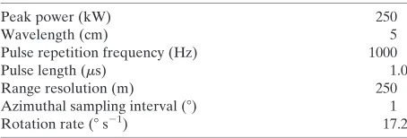
The data were obtained with the Kurnell radar located south of Sydney at 34.018S, 151.238E at an altitude of 64 m MSL. The Kurnell radar is a C band (5-cm wavelength) with a 3-dB beamwidth of 18. The data are collected in polar coordinate format, comprising 360 azimuthal beams each consisting of 596 range gates with a radial spacing of 250 m. The radar operating characteristics are summa-rized in Table 1. Analysis was performed on polar data rather than a transformation to Cartesian coordinates. One volume, consisting of scans at 11 tilt angles (spaced at 0.78, 1.58, 2.58, 3.58, 4.58, 5.58, 6.98, 9.28, 12.08, 15.68, and 20.08) is completed in approximately 5 min. Standard UTC time will be used in this paper; however, for refer-ence, local time (LT) is UTC110 h normally and UTC1 11 h during daylight saving. This radar was chosen for evaluation as it covers one of Australia’s major pop-ulation centers and anaprop is a common occurrence in this location, especially during the summer months when the prevailing subtropical high in the Tasman Sea pro-duces strong temperature and humidity gradients off the Australian eastern coast.

3. Bayes clutter classifier

a. Na€ıve Bayes classifier

In this work a Bayes classifier is developed to distinguish anaprop from precipitation echoes. Bayes’s theorem (e.g., Gelman et al. 2003) relates the a posteriori probability of an object belonging to a particular classcgiven a vector of input observationsx1,. . .,xnand can be written as

P(cjx₁,. . .,x_n)5P(x1,. . .,xnjc)P(c)

P(x₁,. . .,x_n) , (1)

where P(x1,. . .,xnjc) is the conditional probability

distribution (likelihood) of returning a measurementxi

given it belongs to classc,P(c) is the a priori probability of a given class, andP(x1,. . .,xn) is the probability of

obtaining a particular observationxi. The denominator

in Eq. (1) is constant for all classes, making it a constant of proportionality, which can be ignored.

Here, we apply a version of Bayes’s theorem known as the naı¨ve Bayes classifier. The NBC makes the assump-tion that the input measurements xi are conditionally

independent, which greatly simplifies the calculation of the likelihood term in Eq. (1). Assuming the indepen-dence of the input measurements, the likelihood can be expanded as a multiplication of the individual conditional probabilities (Rico-Ramirez and Cluckie 2008) so that

P(cjx₁,. . .,x_n)}P(c)

P

n

i51

P(x_ijc) . (2)

In practice, the independence assumption is often vio-lated; however, the NBC has been shown to be effective even when the independence assumption is known to be false (Friedman et al. 1997). The likelihood PDFs are obtained from training datasets where the classification is known a priori. To obtain the a priori probability of a particular class occurringP(c), a climatological dataset could be used to determine the probability of each class’s occurrence. However, this would induce biases unless the dataset was very large (in theory infinite), and instead we make the assumption that each class is equally likely. For simplicity we will specify two classes: anaprop (AP) and precipitation (PR), henceP(AP)5P(PR)50:5. The number of classes could be extended and in generalP(ci)5

1/(number of classes). Conceptually, the NBC reduces to calculating PDFs of the conditional probabilities, while the classification is determined by maximizing the a posteriori probability. For our purposes, the vector xi corresponds

to a sequence of feature fields, derived from the radar ob-servations, which are described in the next section. b. Feature fields

In this section, we detail the feature fields used as in-put to the NBC. The feature fields can be described as textubased fields that examine various gate-to-gate re-lationships in the retrieved radar fields. The use of feature fields obtained from reflectivity data is advantageous since they require minimal numerical computation. Moreover, they can be applied in a postprocessing capacity, negating any need to upgrade radar hardware or electronics. The three feature fields we will consider are texture of reflec-tivity, ‘‘SPIN,’’ and the vertical profile of reflectivity.

1) TEXTURE OF REFLECTIVITY

The texture of reflectivity (TDBZ) is a measure of the reflectivity difference between adjacent radial reflec-tivity gates. It is computed as (Hubbert et al. 2009; Kessinger et al. 2004)

TDBZ5 "

å

å

(dBZ_i,j2dBZ_i21,j)2

#,

(N3M) , (3) TABLE1. Operating parameters for the Kurnell radar.

Peak power (kW) 250

Wavelength (cm) 5

Pulse repetition frequency (Hz) 1000

Pulse length (ms) 1.0

Range resolution (m) 250

Azimuthal sampling interval (8) 1

Rotation rate (8s21) 17.2

where dBZis the reflectivity measured in a range gate,N is the number of radar beams, andMis the number of radial range gates; the quantityN3Mis referred to as the kernel. The texture of reflectivity is currently used in the U.S. Weather Surveillance Radar-1988 Doppler (WSR-88D) network’s clutter mitigation decision al-gorithm (Hubbert et al. 2009; Kessinger et al. 2004). These formulations include only the radial component in the calculations, although others (e.g., Rico-Ramirez and Cluckie 2008) include the azimuth. Here, we use a formulation similar to that of Hubbert et al. (2009) and average along a kernel of 11 radius gates (centered on the gate of interest) along a single azimuth ray (i.e., N51 andM511). Evaluation of TDBZ in only the radial component has several advantages: 1) it requires less computation time and memory usage; 2) the radar tends to inherently average or smear over azimuths, especially at the fast rotation rates (;178s21) used operationally; and 3) for adjacent azimuths, the distance between measurements increases linearly with range so that TDBZ computed in 2D has range-dependent properties.

2) SPIN

The SPIN feature field is a measure of the number of sign changes in the relative difference of reflectivity between adjacent gates. The difference must be greater than a specified threshold (nominally 2 dBZ), and the result is expressed as a percentage of all possible fluctua-tions within the kernel mask (Steiner and Smith 2002). For example, if three successive gates along a radar ray are considered, each with an associated dBZ value, then in order for a SPIN change to occur, two conditions must be met: 1) there must be a sign change of reflectivity on either side of a specified range gate and 2) the magnitude of the average difference between the range gates preceding and following the range gate of interest must exceed a speci-fied threshold. Mathematically, these conditions can be expressed as (Hubbert et al. 2009)

signfdBZ_i2dBZ_i21g5 2signfdBZ_i112dBZ_ig and (4a) jdBZ_i2dBZ_i21j1jdBZ_i112dBZ_ij

2 .spin threshold .

(4b)

3) VERTICAL PROFILE OF REFLECTIVITY

The vertical profile of reflectivity (VPDBZ) measures the difference between two elevation angles for the same range gate:

VPDBZ5dBZ_u2dBZ_l, (5)

whereuandlrepresent the upper and lower elevation angles, respectively. This field is particularly good at identifying anaprop echoes as they are normally con-fined to the lowest two or three elevations. The bureau’s postprocessing currently uses a measure of VPDBZ to censor echoes due to anaprop; however, it has the un-desired effect of eliminating echoes from shallow strat-iform precipitation.

c. Construction of the conditional probabilities

The application of the NBC requires evaluating PDFs of the a priori conditional probabilities for each class using training datasets. Since we are attempting to dis-tinguish anaprop from precipitation, we specify two classes c1,2, both of which require training data. Data

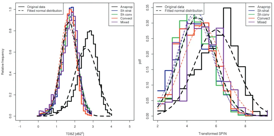
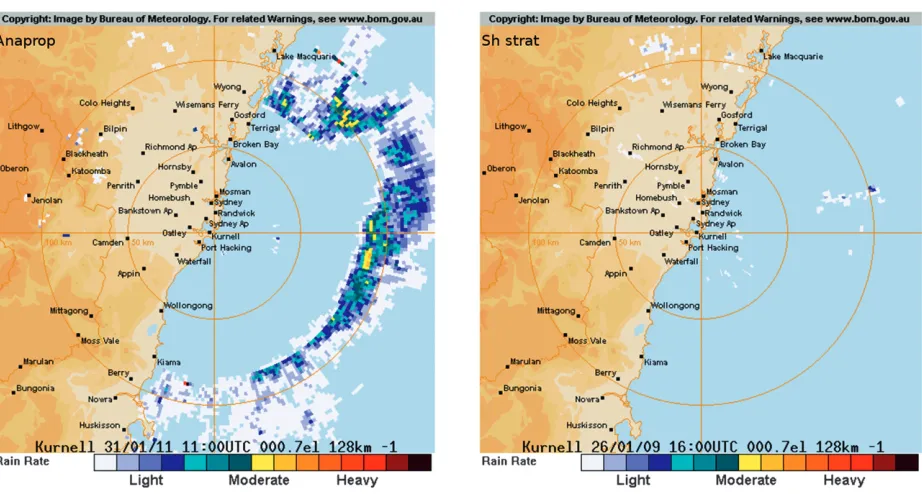
representative of anaprop are shown in Fig. 1, the left-hand side of which shows a plan position indicator (PPI) radar image obtained from the lowest elevation (0.78) of the Kurnell radar at 1100 UTC 31 January 2011. The complete anaprop training dataset spanned the time period 0000–1400 UTC, which consisted of 169 volume scans comprising over 5 million separate reflectivity re-turns (see Table 2). The eastern coast of Australia is indicated by the heavy black line, and many returns can be seen emanating over the ocean. The reflectivity rea-ches magnitudes of 35–40 dBZ, values typical of returns from showers in this location. These returns, however, are not from precipitation but anaprop. This is apparent on examination of the right-hand side of Fig. 1, which shows the range–height indicator (RHI) volume slice at an azimuth of 1008clockwise from north and reveals that returns were only present in the lowest two tilts of the volume scan. The shallow extent of the returns is a strong indicator that they are from anaprop. However, there are occasions when strong precipitation can occur from shallow stratiform clouds; in such situations the vertical extent of reflectivity is not always a good discriminator of anaprop and precipitation. There are also some isolated returns to the west of the radar, which are due to a com-bination of topography and ‘‘clear-air’’1 returns. The clear-air returns are present despite a lower reflectivity threshold of 10 dBZbeing applied to the data (i.e., re-flectivities lower than 10 dBZhave been discarded). The lower threshold of 10 dBZwas chosen, as this is about the lowest reflectivity that signifies the onset of precipitation

1_{Clear-air returns are returns measured when there are no}

(Knight and Miller 1993). It is apparent that if the anaprop signals were assimilated, the NWP model would attempt to create precipitation where none was present. The aim therefore is to identify and remove echoes from anaprop.

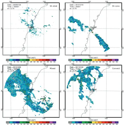
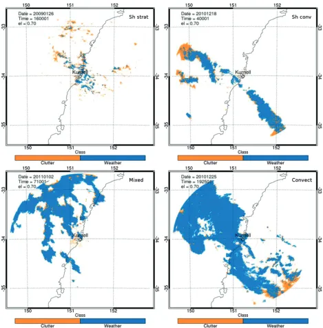
For the construction of the conditional PDFs for the precipitation class, four separate precipitation scenarios were chosen: shallow stratiform rain where cloud tops were below the freezing level and precipitation was generated by warm rain processes, a line of shallow convection with cloud tops below 5 km, deep isolated continental convection, and widespread stratiform rain with embedded convection. These will be referred to as Shallow, Sh conv, Convect, and Mixed, respectively. The reasons for these choices were twofold: 1) to capture a wide variety of meteorological cases and 2) to increase sampling statistics. Radar images (PPIs) representative of each of the scenarios are shown in Fig. 2. A visual comparison of anaprop with the shallow convection case (upper-right panel of Fig. 2) indicates that there is little information in the reflectivity field to distinguish them. Histograms of reflectivity (not shown) confirm this; in fact, there is little information in the reflectivity field (of a PPI) to distinguish each of the precipitation examples (except perhaps shallow stratiform rain) from anaprop. Therein lies the problem of automated detection of anaprop from the reflectivity field alone.

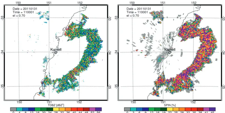
More information can be gained from examining the feature fields, TDBZ and SPIN, which are shown for anaprop in Fig. 3. Immediately apparent is the lack of correspondence in structure of the feature fields com-pared with that of reflectivity (i.e., small/large values of reflectivity do not show up as small/large values of TDBZ or SPIN). TDBZ and SPIN are shown for the precipitation cases in Figs. 4 and 5, respectively. Again, the feature fields are relatively homogeneous through strong gradients in reflectivity; however, it is evident that both TDBZ and SPIN are 1) skewed to larger values and 2) noisier for anaprop than for the meteo-rological events. Furthermore, there is little distinction in the feature fields between each of the precipitation cases. These observations suggest that TDBZ and SPIN FIG. 1. (left) PPI obtained from the Kurnell radar at 1100 UTC 31 Jan 2011 (2200 LT). Some returns are of the order 35–45 dBZ, which is also typical of showers in this location. (right) RHI obtained at an azimuth of 1008from the north. Returns are prevalent between the 80-and 130-km range; however, they are only present in the lower two elevations, signifying their source is from anaprop. Only reflectivities above 10 dBZare shown.

TABLE2. Summary of time periods, number of radar volumes, and number of unique reflectivity samples used for the training dataset.

Meteorological type

Time period (UTC)

No. of volumes

No. of dBZ

samples

Anaprop 0000–1400 169 5 089 099

Sh strat 1420–2315 107 1 405 144

Sh conv 0200–0500 37 664 291

Convect 0230–0730 61 1 007 198

Mixed 1430–2300 103 6 263 822

are efficient at distinguishing anaprop from precipita-tion and independent of the meteorology producing precipitation.

For the purposes of constructing the conditional PDFs, time periods were chosen where the precipitation sce-narios exemplified in Fig. 2 were applicable throughout. These periods were chosen subjectively by examining sequences of radar images and choosing a subset of contiguous retrievals such that the precipitation was similar (in the sense of areal extent and type) in each volume throughout the interval. Only samples from the lowest tilt of the volume scan were used to construct the PDFs. Combined, the precipitation samples con-sisted of 308 volumes comprising over 9 million separate

reflectivity samples. Histograms of the feature fields were then constructed for each of the precipitation scenarios and for anaprop. They are shown in Fig. 6 and represent the conditional probabilities on the right-hand side of Eq. (2).

d. Transformation of the conditional PDFs

To implement the conditional PDFs presented in the preceding section would require the use of a lookup table. For instance, the feature fields could be evaluated and a probability determined (via the lookup table) of that measurement occurring based on whether the clas-sification was that of anaprop or precipitation. For op-erational purposes, however, this is unfeasible because of FIG. 2. PPI radar reflectivity displays of the meteorological cases chosen for the training dataset. Clockwise from

the top left depicts shallow stratiform (Sh strat), a shallow line of convection (Sh conv), deep intense lines of isolated convection (Convect), and widespread stratiform rain with embedded convection (Mixed). Only reflectivities above 10 dBZare shown.

computational limitations. To facilitate the implementa-tion of the classifier in an operaimplementa-tional setting, it would be beneficial if the conditional probability distributions presented in Fig. 6 were parameterized by a mathemati-cal distribution. This is achievable by applying a trans-formation to the data. One that is well established within the statistical literature is the Box–Cox transformation, which can map data to a nearly normal distribution via a power transform (Wilks 2011). This has the advantage that the conditional PDFs can be completely described by the meanmand standard deviations, requiring minimal computation.

The Box–Cox transformation is described mathe-matically by

y(l)5

8 > < > :

yl21

l , if l6¼0 logy, if l50

, (6)

where y is the measured variable and l is the trans-formation parameter. The value of l is evaluated by maximizing the logarithm of the likelihood function (Wilks 2011)

f(y,l)5 2n 2ln

(

å

i51

[y_i(l)2y(l)]2 n

)

1(l21)

å

n

i51

ln(y_i) ,

(7)

where y(l) is the arithmetic mean of the data. In this case, y corresponds to a vector of observations

y5(y1,y2,y3), where the elements of the vector are

given by the feature fields. The PDF for VPDBZ is already approximately normal (see Fig. 6) and so the transformation was only applied to the TDBZ and SPIN feature fields.

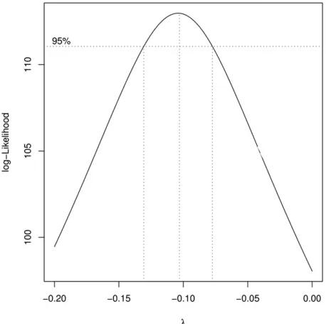
The log-likelihood functions for the TDBZ and SPIN feature fields were evaluated and the calcula-tions for the TDBZ field of anaprop are shown in Fig. 7. The maximum of this parabolic function pro-vides the optimal value oflfor insertion to Eq. (6) so as to transform the PDFs shown in Fig. 6 to an ap-proximately normal distribution. Similar calculations were performed for all meteorological scenarios and each feature field, the results of which are summarized in Table 3. Since it cannot be known a priori what the prevailing meteorology is, an average value applicable to all precipitation caseslweatherwas evaluated. These

values are listed in the right-hand side of Table 3 and were used to transform the conditional PDFs of Fig. 6 via Eq. (6).

The resulting transformed PDFs are shown in Fig. 8. As was found prior to the application of the Box–Cox transformation, the PDFs are approximately equal for all precipitation scenarios, and they are distinct from anaprop for both TDBZ and SPIN. It is also noted that the Box–Cox transformation has been successful at transforming the PDFs to approximately normal distri-butions. The original TDBZ and SPIN fields were reevaluated from the training dataset and the Box–Cox transformation applied to it. The m andsof the data were then evaluated via a two-pass algorithm:

FIG. 3. The texture (TDBZ) and SPIN fields for the anaprop case shown in Fig. 1. Only reflectivities above 10 dBZ

have been included in the calculations.

m5

å

i51

x_i/n and

s5

å

n

i51

(x_i2m)2

n21 . (8)

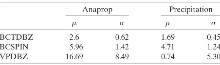
These values are summarized in Table 4. The Gaussian distributions described by these two parameters were calculated and are plotted in Fig. 9 and also overlaid with the histograms of Fig. 8. The Gaussian distributions calculated directly from the mean and standard de-viation of the data very closely overlay the PDFs of the original data, and therefore, to a close approximation, the conditional PDFs can be parameterized via the mean and standard deviation of the Box–Cox transformation of

the respective feature fields. We label these feature fields BCTDBZ and BCSPIN.

e. Independence of the feature fields

The linear independence of the input feature fields is one of the key assumptions of the NBC. Despite this assumption, it has been proven to be effective even when the assumption of independence is violated (Friedman et al. 1997). However, it is worthwhile to examine the independence assumption between each of the feature fields. Pearson’s correlation coefficients were calculated for each combination of the original and Box–Cox transformed feature fields. The results are summarized in Table 5. The VPDBZ field is either un-correlated or very weakly un-correlated with TDBZ and SPIN; the same is true for the Box–Cox transformed FIG. 4. The texture feature field (TDBZ) for each of the precipitation cases as in Fig. 2. Only reflectivities above

10 dBZhave been included in the calculations.

counterparts BCTDBZ and BCSPIN. This may be ex-pected as TDBZ and SPIN are measures of fluctuations of the reflectivity in a horizontal plane, while VPDBZ measures fluctuations in the vertical plane. However, the correlation coefficient for TDBZ and SPIN indicates a modest correlation (0.36) and a slightly greater cor-relation (0.48) after transformation. The corcor-relation between TDBZ and SPIN is most likely due to each of them quantifying the fluctuation of the reflectivity field. The increased correlation between TDBZ and SPIN after transformation (for both anaprop and precipita-tion) is most likely due to the decreased range of the variables after transformation. For example, SPIN has values in the range [0, 100], whereas BCSPIN is in the range [2, 9]. Moreover, the Box–Cox transformation reduces larger values by a greater proportional amount

than smaller values, thereby increasing the covariance of a feature field (Wilks 2011).

4. Results and discussion

a. Varying input feature fields on the training dataset

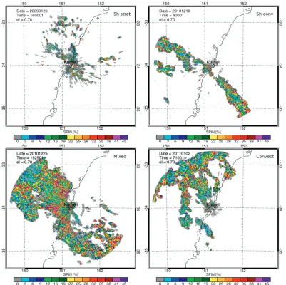
It was stated in section 3 that the NBC implicitly as-sumes independence of the input feature fields; how-ever, a modest degree of correlation between TDBZ and SPIN was also demonstrated. In this section, we examine how the NBC performs using differing com-binations of the feature fields and determine if the correlation between TDBZ and SPIN affects the pre-dictive power of the NBC. To illustrate this, we inves-tigated all possible combinations of TDBZ, SPIN, and FIG. 5. The SPIN feature field for each of the precipitation cases as in Fig. 2. Only reflectivities above 10 dBZhave

been included in the calculations.

VPDBZ as input feature fields to the NBC (BCTDBZ, BCSPIN, VPDBZ, BCTDBZ–BCSPIN, TDBZ–VPDBZ, SPIN–VPDBZ, and TDBZ–SPIN–VPDBZ) and applied them to the case presented in Fig. 1 (which was repre-sentative of the training dataset for anaprop). A visual inspection was made to determine the least and most effective combinations, which are shown in Fig. 10. Returns classified as precipitation are colored blue while those from anaprop are colored orange. The use of BCTDBZ alone proved the least effective while the BCTDBZ–VPDBZ combination proved to the most ef-fective classifier of anaprop. In general, VPDBZ had the greatest discriminatory power (combined with BCTDBZ or BCSPIN) for anaprop and was even quite effective if used as the sole feature field. The use of either BCTDBZ or BCSPIN alone was least effective since many range gates that were anaprop were misclassified as precipitation.

FIG. 6. Probability distribution functions of the feature fields TDBZ, SPIN, and VPDBZ. PDFs are shown for each of the me-teorological situations and for anaprop. These PDFs represent the likelihood function in the Bayes formula [Eq. (2)]. Note the loga-rithmic axes for TDBZ. Only reflectivities above 10 dBZhave been included in the calculations.

FIG. 7. The log-likelihood as a function ofl[see Eq. (7)]. The value ofl, which maximizes the log-likelihood function, provides the best value to transform the data to an approximately normal distribution via Eq. (6). The dotted lines represent the 95% con-fidence interval forl. This curve is the log-likelihood function evaluated for the TDBZ field of the anaprop case. Values for TDBZ and SPIN for each case are presented in Table 3.

TABLE3. Calculated values oflfor the Box–Cox transformation described by Eq. (6) for anaprop and each of the precipitation cases. The last column shows the average value oflfor all pre-cipitation cases combined.

Anaprop Sh strat

Sh

conv Convect Mixed lprecipitation

TDBZ 20.11 20.34 20.2 20.22 20.24 20.25

SPIN 0.3 0.25 0.25 0.26 0.29 0.26

Including all three feature fields resulted in little or no improvement over using either BCTDBZ or BCSPIN combined with VPDBZ.

The possible NBC feature field combinations were evaluated using the precipitation cases from the train-ing dataset. In all cases, the TDBZ–VPDBZ combi-nation obtained similar results to the application of all three feature fields, while the SPIN–VPDBZ com-bination performed poorly. The addition of the SPIN feature field may not have enhanced the efficacy of the NBC because of the independence assumption of TDBZ and SPIN being violated. That the SPIN–VPDBZ combination performed worse than the TDBZ–VPDBZ combination may be due to the application of the kernel in Eqs. (3) and (4) being only evaluated in the radial direction. A kernel size of 20 was chosen, so as to allow a sufficient dynamic range in the evaluation of the SPIN (a kernel size of 20 will give a minimum discrete interval of 5% in the evaluation of SPIN). However, a kernel size of 20 equates to a radial range of 5 km, which may have the unintended consequence of smearing over precip-itation and nonprecipprecip-itation pixels. The inclusion of azimuths in the evaluation of SPIN, which will enable the kernel size to be kept the same while decreasing the ra-dial extent, is needed to evaluate the effectiveness of evaluating SPIN in one dimension only. Despite this, it appeared that using TDBZ and VPDBZ gave similar results to the application of all three feature fields and for this reason the BCTDBZ–VPDBZ combination will be used to present the NBC results herein.

The image, which was transmitted for public display by the bureau corresponding to the anaprop presented in Fig. 1, is shown in the left-hand side of Fig. 11. The NBC provides a substantial improvement over the cur-rent clutter mitigation system employed at the bureau. The current scheme uses basic thresholds of reflectivity and vertical height to censor data. However, in the im-age shown, the reflectivity and height thresholds were exceeded, allowing them to be included. The problem becomes more pronounced at greater distances from the radar because beam propagation causes the beam to be above the minimum height threshold once a certain range is reached.

b. Verification of the classifier

After conducting a visual evaluation of the best combination of feature fields to input to the NBC, the FIG. 8. Probability distribution functions of the feature fields TDBZ and SPIN after transformation according to the Box–Cox power law

given by Eq. (6). Note that the distributions are now approximately normal.

TABLE 4. Mean m and standard deviation s of the feature fields for anaprop and precipitation. The values in the precipitation column are an average of each of the precipitation scenarios. They were obtained by applying the Box–Cox transformation to the feature fields of the training data and then computing_mand_sof the transformed distribution.

Anaprop Precipitation

m s m s

BCTDBZ 2.6 0.62 1.69 0.45

BCSPIN 5.96 1.42 4.71 1.24

VPDBZ 16.69 8.49 0.74 5.30

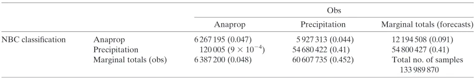
performance of the NBC was quantified. To achieve this we applied the NBC to each of the training datasets, which we assumed a priori consisted entirely of either anaprop or precipitation samples. The data were used to construct the conditional probability PDFs presented in Fig. 8 and therefore, if the NBC was perfect, would classify each pixel correctly. The total number of pixels classified as either anaprop or precipitation was calcu-lated for each of the training datasets and the results are presented as a contingency table in Table 6. The num-bers differ from those in Table 2 because all of the pixels in a volume were used to construct the contingency ta-ble, while only those from the lowest tilt were used to train the NBC. The raw values are presented above and the proportional values are presented below in the brackets. There are many different skill scores that can be derived from the contingency table; however, the dimensionality of the table is three and all the infor-mation contained in it can be summarized with three statistics (Wilks 2011). Three that are commonly used are the hit rate [H5a/(a1c)], the false alarm rate [F5b/(b1d)], and the base rate [P(c) or sample cli-matological relative frequency] of the class in question. Each of these scalar attributes can be quoted for each class (i.e., anaprop or precipitation), but we will quote only the values for anaprop:H50.981,F50.098, and P(c)50.095. This means that about 98% of the anaprop pixels were correctly detected, and about 10% of the precipitation pixels were misclassified as anaprop. The

sample climatological relative frequency of anaprop was about 10%, which is probably substantially larger than the actual climatological frequency of anaprop. In other words, the NBC is very good (98%) at classi-fying anaprop correctly; however, 10% of the time it incorrectly classifies a precipitation pixel as anaprop. For the purposes of QPE or NWP assimilation, this is a more desirable characteristic than the opposite (i.e., misclassifying 10% of anaprop as precipitation). c. Application to the training dataset precipitation

cases

The results of applying the NBC to the precipitation cases, using the BCTDBZ–VPDBZ feature fields as FIG. 9. As in Fig. 8, including the best-fit normal curves determined from the mean and standard deviation of the Box–Cox

transformed training datasets.

TABLE5. Pearson coefficient of correlation for anaprop con-ditions and the differing precipitation cases. All possible co-efficients are shown for the original feature fields (TDBZ, SPIN, and VPDBZ) and the Box–Cox transformed values (BCTDBZ, BCSPIN, and VPDBZ).

Anaprop Sh strat

Sh

conv Convect Mixed

TDBZ–SPIN 0.36 0.36 0.37 0.28 0.46

TDBZ–VPDBZ 20.01 0.03 20.15 20.05 20.1 SPIN–VPDBZ 0.02 20.03 20.09 20.02 20.06

BCTDBZ–BCSPIN 0.48 0.46 0.49 0.42 0.53

discriminators, are shown in Fig. 12. For the shallow stratocumulus case (top left) the NBC has identified most (;70%) reflectivities larger than about 15 dBZ as precipitation. The formation of precipitation-sized droplets is indicated at radar reflectivities of about

5–10 dBZfor a C-band radar (Knight and Miller 1993), so the NBC has been particularly effective at identifying the shallow precipitation bands within these stratocu-mulus. We also note that the current method employed at the bureau to eliminate anaprop, which relies solely FIG. 10. The results of the NBC applied to the anaprop training dataset presented in Fig. 1. (left) The image was

obtained using BCTDBZ only for classification, while (right) the image used BCTDBZ and VPDBZ.

FIG. 11. Images transmitted for public display using the bureau’s current clutter mitigation system. The images correspond to the anaprop data presented in Fig. 1 and the shallow stratiform case presented in Fig. 2. It can be seen that the current system is ineffective at removing anaprop, especially far from the radar, while it also removes many genuine precipitation pixels, especially close to the radar.

on examining the vertical profile of reflectivity, rejected these echoes in near entirety as anaprop (see the right-hand side of Fig. 11). This was because the precipitation was mainly confined below the height threshold de-signed to eliminate anaprop. The NBC represents a substantial improvement for the identification of shal-low precipitation. Shalshal-low cumulus convection is also well distinguished; however, some precipitation echoes, especially those at the edge of the radar volume, have been incorrectly classified as anaprop. This is due to the spread of the radar beam with distance and the use of VPDBZ as a classifier. In this case, cloud-top height was between 4 and 5 km and at large distances from the ra-dar; two vertically aligned range gates were sufficiently large to overshoot cloud top, resulting in a VPDBZ value greater than zero, which is typical of anaprop (see Fig. 6). We note that the NBC using BCTDBZ only as the input feature field identified all of the returns as precipitation suggesting that, in the case of shallow precipitation, the use of BCTDBZ alone may perform better. The inclusion of BCSPIN degraded the perfor-mance of the NBC. However, since it is not known a priori what the source of returns is and the NBC cannot adapt its input feature fields accordingly, the use of the most effective combination over all precipitation types (BCTDBZ–VPDBZ) is preferable. The classification of the deeper precipitation, whether stratus or convective in nature (Convect and Mixed), has been mostly (88% and 94%, respectively) successful. Given that the cur-rent numerical weather prediction model used at the bureau—the Australian Community Climate and Earth-System Simulator (ACCESS; Puri et al. 2013)—has a grid spacing of 5 km, the raw radar reflectivity needs to be thinned (using superobservations); this level of accuracy is most likely suitable for data assimilation or QPE/QPF (Weng and Zhang 2012).

d. Application to a case of rain embedded in anaprop

We now evaluate the NBC on a case other than the training dataset. Consider Fig. 13, which is a particularly interesting example as the image contains returns from both anaprop and precipitation. The returns in the northeast quadrant of the image are from anaprop,

while those in the southeast are from convective storms. This becomes apparent when examining the PPI ob-tained at the second radar elevation (top right), where the returns originating from anaprop have disappeared as the radar beam is no longer internally reflected at the temperature and humidity inversion. This is further em-phasized when the RHIs at 408and 1128(reconstructed from the volume scan) are examined; the RHI at 408only has returns in the lowest elevation, while the RHI at 1128 indicates the presence of a well-developed convective storm containing reflectivities greater than 25 dBZ ex-tending above 7 km. The simultaneous presence of both anaprop and precipitation in the same image provides a useful example with which to evaluate the efficacy of the NBC.

Figure 14 shows the results of applying the NBC to this scene using BCTDBZ and VPDBZ as input fea-ture fields. The PPI images (top row) show that the NBC is effective at distinguishing anaprop from pre-cipitation; however, some precipitation pixels have been misclassified as anaprop. This is further illustrated by the RHI images (bottom row) again at 408and 1128, which indicate that while the NBC has positively iden-tified anaprop, some precipitation signals have been misclassified.

e. The effect of the reflectivity threshold

For the preceding analysis, the minimum reflectivity threshold used (for the evaluation of the feature fields, their conditional PDFs, and for classification) was 10 dBZ, which, for a C-band radar, is near the value one would expect for the initiation of precipitation-sized droplets (Knight and Miller 1993). If values below this are included, then clear-air returns from insects and Bragg scattering from humidity gradients in the atmo-sphere become enhanced. The effect of setting a mini-mum reflectivity threshold at 230 dBZ (the smallest value returned by the radar) is shown in the left panel of Fig. 15. There is an increased number of returns close by the radar, especially over land, most likely due to the presence of insects and Bragg scattering. Condi-tions conducive to Bragg scattering would be expected since the same temperature and humidity gradient that TABLE6. Contingency table constructed from the anaprop and precipitation training datasets. A minimum reflectivity threshold of 10 dBZ

was applied. The raw values are presented first, and the proportional values are given after in parentheses.

Obs

Anaprop Precipitation Marginal totals (forecasts)

NBC classification Anaprop 6 267 195 (0.047) 5 927 313 (0.044) 12 194 508 (0.091) Precipitation 120 005 (931024_{) 54 680 422 (0.41) 54 800 427 (0.41)}

Marginal totals (obs) 6 387 200 (0.048) 60 607 735 (0.452) Total no. of samples 133 989 870

produced anaprop over the sea would be prevalent, although to a lesser extent, over land. Despite the extra returns, when the reflectivity threshold is lowered the NBC did not classify most of the extra returns as pre-cipitation. Since data below 10 dBZwere excluded during development of the NBC, it is interesting that most of the clear-air echoes have been classified as anaprop. Ex-amination of a time sequence of images revealed that the echoes over land close to the radar (corresponding

to those classified as precipitation) were due to Bragg scattering while those farther away (classified as anaprop) were caused by insects present after sunset. The NBC may therefore also prove useful in identifying insects and boundary layer humidity gradients; however, this will require further investigation. Nevertheless, for the purposes of data assimilation and QPE, setting a re-flectivity threshold near 10 dBZ is advisable and will help mitigate this problem. However, the use of the FIG. 12. The results of the NBC applied to the precipitation cases from the training dataset. The original reflectivity images are

shown in Fig. 2.

Doppler wind field (e.g., Rennie et al. 2011) is advisable to identify insect echoes and such research is being undertaken concurrently at the bureau. Furthermore, software is being developed within the bureau that will enable selecting regions of interest and subjectively defining an a priori class to them to determine if and how PDFs of feature fields for insects (for instance) differ from those of anaprop.

f. Application to radars other than Kurnell

It is feasible that the texture and SPIN variables may be sensitive to radar operating characteristics such as wavelength, beamwidth, height above mean sea level (MSL), and range resolution. The Kurnell radar (64 m MSL) is ideally situated to test this hypothesis as two bureau radars are located to the north and south of it, each with differing operating characteristics. The Terrey Hills radar is an S-band (10 cm) 18 beamwidth radar located about 40 km to the north of the Kurnell radar at 195 m MSL, while the Wollongong radar is an S-band 28 beamwidth radar located about 55 km to the south at

449 m MSL. Together, the radars are a combination of 5- and 10-cm wavelengths and 18 and 28 beamwidth operating parameters.

Figure 16a is an example of shallow maritime con-vection and anaprop observed by each of the radars at approximately the same time. The same gross features are evident with many convective elements present over the ocean. The convection was very shallow and con-fined mostly below 4 km altitude. Consider the small convective element just east of the Kurnell radar, which is circled. It is clearly visible in all three radars; much anaprop is evident in the Kurnell and Wollongong ra-dar images, however. Figure 16b shows the results of applying the NBC to the PPIs. It can be seen that the anaprop surrounding the convection in the Kurnell and Wollongong images has been correctly distinguished. It is encouraging that the NBC has managed to perform well when applied to radars with different operating characteristics and gives us confidence that the NBC can be directly applied to other radars around the country. It is unclear why more anaprop is present in the Kurnell FIG. 13. An example of anaprop and a convective storm obtained from the Kurnell radar on 22 Jan 2010. Anaprop

is present in the northeast and a convective storm in the southeast. (top left) A PPI image obtained at the lowest elevation (0.78); (top right) a PPI image obtained at the next highest elevation (1.58). Note the absence of anaprop in the higher elevation. (bottom left) An RHI obtained at an azimuth of 408through the anaprop; (bottom right) an RHI at 1128, showing the presence of a convective system extending to nearly 10-km height.

and Wollongong radars compared to Terrey Hills. It may be due to the altitude of the radar; however, Terrey Hills is at an altitude midway between the other two indicating no obvious decrease in anaprop as a function of the height of the radar as may be ex-pected. The radar beamwidth may be a contributing factor since Wollongong (with a 28 beamwidth) ex-hibits a greater amount of anaprop compared with the other two radars. In particular, tests of the NBC on ra-dars at other locations around Australia reveal that the feature fields may be susceptible to beamwidth and range resolution. Another factor that may influence the NBC may be the climatic region for which it was tuned; that is, it may not perform so well in the tropical north of the country or in the temperate regions farther south. These points need further examination and will be the focus of future studies of the applicability of the NBC to the bureau’s radars.

g. A strength of classification index

The NBC has proven successful in distinguishing anaprop from precipitation and would be a useful tool for an operational forecaster or for the layperson viewing

publicly available radar images. However, for the pur-poses of assimilation or QPE/QPF, it would prove beneficial to have some knowledge of the confidence one has in data being precipitation. This could take the form of an absolute probability by evaluating the a priori probability for each classP(c); however, as detailed in section 3 that would require a climatological dataset to determineP(c) for each bin in the radar volume, which is contrary to the efficiency inherent in using the NBC. To this end, we constructed an SOC. The SOC is a measure of the relative proportion by which the condi-tional probability [the left-hand side of Eq.(2)] of pre-cipitation exceeds that of anaprop as a proportion of the maximum possible difference after both of the a poste-riori probabilities have been scaled to be in the range [0, 1]. Mathematically this is expressed as

SOC5 P(prjxi) maxfP(prjx_i)g2

P(apjx_i) maxfP(apjx_i)g,

where, maxfP(cjx_i)g5max

(

P

)

. (9)

FIG. 14. The results of the NBC applied to Fig. 13 using BCTDBZ and VPDBZ as input feature fields. The NBC has classified the anaprop correctly, completely eliminating the returns in the northeast; however, some pixels that are returns from precipitation have been incorrectly classified as clutter.

The SOC therefore scales in the range [21, 1], where 0 indicates that the likelihood of precipitation and anaprop is equal, and 1 indicates that the likelihood of anaprop was zero and for precipitation was a maximum (which is unity after scaling). The sign of this number is determined by the order of the terms in Eq. (9) and an equivalent index could be constructed for anaprop. In practice, if a pixel has been identified as anaprop, then it is discarded as we are interested only in the SOC for precipitation, that is, values in the range [0, 1].

An example of the evaluation of the SOC applied to the precipitation training datasets is shown in Fig. 17. The color scale has been truncated at 0.5 as most values appear to be confined below this. To quantify the range of the SOC, PDFs of the training set data were con-structed and are presented in Fig. 18. The SOC index is mainly confined to values below about 0.5. The PDFs of SOC exhibit a maximum at the first bin (0–0.05) showing that the majority of pixels identified as pre-cipitation have only had a slightly higher a posteriori probability of precipitation than anaprop. However, the PDFs for each of the weather cases are relatively flat above an SOC of about 0.05. It is anticipated that the assimilation and QPE communities would be able to set a minimum value of the SOC, above which data pixels would be accepted. Increasing the SOC results in a decrease in the amount of information that can be assimilated; however, the flatness of the PDFs in Fig. 18 suggests that the information loss is approximately linear above an SOC threshold of about 0.05.

5. Summary and conclusions

In this study, a naı¨ve Bayes classifier was developed and tested. The NBC is an extension of Bayes’s theorem, which classifies radar echoes into two classes,c1andc2,

based on a series of feature vectors, x1,. . .,xn, by

maximizing the a posteriori probability p(cijxi). The

classes were designated to be either anomalous propaga-tion (anaprop) or precipitapropaga-tion, and the feature fields in-vestigated were the texture of reflectivity (TDBZ), spin change variable (SPIN; Steiner and Smith 2002), and vertical profile of reflectivity (VPDBZ).

The NBC is a supervised learning technique, which requires a training dataset of examples in which the classification is known a priori. The training dataset consisted of five subclasses: one of anaprop and four distinct precipitation regimes consisting of shallow strat-iform, shallow convection, deep convection, and deep stratiform precipitation with embedded convection. Probability distribution functions of the feature fields were evaluated for anaprop and each of the pre-cipitation subclasses. The PDFs of the prepre-cipitation subclasses were found to be similar despite distinct meteorological forcing mechanisms. Moreover, the PDFs of the feature fields for anaprop were distinct from the PDFs of the precipitation subclasses, suggesting that they convey information that allows the categorization of precipitation and anaprop.

The feature field PDFs were found to be nonnormal, which, if used in their native form, would require the use of look-up tables to evaluate the conditional probability FIG. 15. (left) PPI image of mixed anaprop and precipitation using a minimum reflectivity threshold of230 dBZ.

Note the increase in returns over land close to the radar compared to Fig. 13. These returns were most likely due to Bragg scattering. (right) Results of the NBC using230 dBZas the minimum reflectivity threshold.

in Bayes’s theorem. To parameterize the conditional PDFs they were transformed to approximately normal distributions via a Box–Cox transformation, which al-lowed them to be specified completely via the mean and standard deviation.

All (seven) possible combinations of the feature fields were investigated on the training datasets to evaluate the most effective combination, which was found to be TDBZ and VPDBZ. The use of all three feature fields did not, as a rule, add any benefit to the NBC and in some cases caused it to perform worse. This was attrib-uted to TDBZ and SPIN not being linearly independent as they are both measures of the variability of the reflectivity field. When considered individually, VPDBZ was found to be the most effective feature field at dis-tinguishing anaprop from precipitation.

The NBC was then applied to an independent case where precipitation and anaprop were present in the same region. The BCTDBZ–VPDBZ combination of feature fields proved most effective at classifying pixels correctly. Some pixels were incorrectly classified, but

given the current data resolution required for purposes of data assimilation or QPE these errors were consid-ered minimal. Some sensitivity to the reflectivity thresh-old was found, whereby returns from clear air appeared as the threshold was decreased. However, when the threshold was set at a reasonable level to distinguish most clear-air returns from the smallest precipitation-sized drops, (around 5 dBZ for a C-band radar) this problem was circumvented. The NBC, however, shows some promise in being able to distinguish Bragg echoes from insect echoes.

The NBC was extended via a strength of classification (SOC) index, which was constructed as a measure of the confidence with which a pixel was classified as pre-cipitation. It was formulated as the difference of the scaled (to be in the range [0, 1]) a posteriori probabilities of weather and anaprop expressed as a proportion of the maximum possible difference. Formulated in this way, the SOC has a range [21, 1]; however, since we are only interested in determining the confidence we have in identifying precipitation pixels, negative values (which FIG. 16. Shallow maritime cumulus convection observed with three different radars. (a) The reflectivity images; (b) the corresponding classification images obtained using the NBC. The three radars (Terrey Hills, Kurnell, and Wollongong) each have a differing wavelength and/or beamwidth. The NBC has performed well on data obtained with each radar despite having been trained with data obtained from the Kurnell radar.

correspond to anaprop) are discarded so the SOC is in the range [0, 1]. In practice, however, it was found that the SOC was confined to values below about 0.5. The PDF of SOC exhibited relatively constant values in the range [0.05, 0.5]. The SOC can be used to remove data below a specified threshold before processing in appli-cations such as assimilation or QPE. Because of the relatively constant values of the PDF of SOC, increasing the SOC threshold in the range [0.05, 05] will result in an approximately linear decrease in the amount of ac-cepted data.

The use of an NBC was found to be an effective method of distinguishing anaprop from precipitation. It should also be noted that it was effective using only a few derived feature fields and single-polarization data. This

makes it useful for the bureau’s radar network, which currently consists of single-polarized radars, a few of which have Doppler capability. At present, only cor-rected reflectivity and Doppler velocity are transmitted from the radar; however, plans exist to extend this to include spectrum width and uncorrected reflectivity. The inclusion of these variables and their associated feature fields should improve the capability of the NBC. At present, no dual-polarized radars exist in the bureau’s operational network; however, the extension of the NBC to include polarimetric variables could be readily accomplished. The bureau now owns the CP2 dual-polarimetric research radar (previously owned by NCAR) so we plan to investigate the use of the NBC with polarimetric variables in the future.

FIG. 17. The strength of the classification index evaluated for each of the precipitation cases from the training dataset. A larger value indicates a larger confidence that a pixel is precipitation.

Acknowledgments. We thank Drs. Alain Protat and Susan Rennie for informative discussions on many as-pects of this work and also for providing feedback on an early version of the manuscript. The thoughtful and constructive comments of the three anonymous re-viewers proved particularly helpful, especially with the development of the SOC index.

REFERENCES

Alberoni, P. P., T. Andersson, P. Mezzasalma, D. B. Michelson, and S. Nanni, 2001: Use of the vertical reflectivity profile for identification of anomalous propagation.Meteor. Appl., 8, 257–266.

Bech, J., B. Codina, and J. Lorente, 2007: Forecasting weather radar propagation conditions.Meteor. Atmos. Phys.,96,229– 243.

Brooks, I. M., A. K. Goroch, and D. P. Rogers, 1999: Observations of strong surface radar ducts over the Persian Gulf.J. Appl. Meteor.,38,1293–1310.

Doviak, R. J., and D. S. Zrnic, 1984:Doppler Radar and Weather Observations.Academic Press, 562 pp.

Faures, J. M., D. C. Goodrich, D. A. Woolhiser, and S. Soorooshian, 1995: Impact of small-scale spatial variability on runoff simula-tion.J. Hydrol.,173,309–326.

Friedman, N., D. Geiger, and M. Goldszmidt, 1997: Bayesian network classifiers.Mach. Learn.,29,131–163.

Gelman, A., J. B. Carlin, H. S. Stern, and D. B. Rubin, 2003:

Bayesian Data Analysis.Chapman & Hall/CRC, 696 pp.

Gourley, J. J., P. Tabary, and J. Parent du Chatelet, 2007: A fuzzy logic algorithm for the separation of precipitating from non-precipitating echoes using polarimetric radar observations.

J. Atmos. Oceanic Technol.,24,1439–1451.

Grecu, M., and W. F. Krajewski, 2000: An efficient methodology for the detection of anomalous propagation echoes in radar reflectivity data using neural networks. J. Atmos. Oceanic Technol.,17,121–129.

Hubbert, J. C., M. Dixon, and S. M. Ellis, 2009: Weather radar ground clutter. Part II: Real-time identification and filtering.

J. Atmos. Oceanic Technol.,26,1181–1197.

Keeler, R. J., and R. E. Passarelli, 1990: Signal processing for at-mospheric radars.Radar in Meteorology,D. Atlas, Ed., Amer. Meteor. Soc., 199–229.

Kessinger, C., S. Ellis, J. van Andel, J. Yee, and J. Hubbert, 2004: Current and future plans for the AP clutter mitigation scheme. Preprints,20th Int. Conf. on Interactive Information and Pro-cessing Systems (IIPS) for Meteorology, Oceanography, and Hydrology,Seattle, WA, Amer. Meteor. Soc., 12.5. [Available online at https://ams.confex.com/ams/84Annual/webprogram/ Paper73376.html.]

Knight, C. A., and L. J. Miller, 1993: First radar echoes from cu-mulus clouds.Bull. Amer. Meteor. Soc.,74,179–188. Krajewski, W., and B. Vignal, 2001: Evaluation of anomalous

propagation echo detection in the WSR-88D data: A large sample case study.J. Atmos. Oceanic Technol.,18,807–814. Lakshmanan, V., A. Fritz, T. Smith, K. Hondl, and G. Stumpf,

2007: An automated technique to quality control radar re-flectivity data.J. Appl. Meteor. Climatol.,46,288–305. Luke, E. P., P. Kollias, K. L. Johnson, and E. E. Clothiaux, 2008: A

technique for the automatic detection of insect clutter in cloud radar returns.J. Atmos. Oceanic Technol.,25,1498– 1513.

Meischner, P., C. Collier, A. Illingworth, J. Joss, and W. Randeu, 1997: Advanced weather radar systems in Europe: The COST 75 action.Bull. Amer. Meteor. Soc.,78,1411–1430.

Moszkowicz, S., G. J. Ciach, and W. F. Krajewski, 1994: Statistical detection of anomalous propagation in radar reflectivity pat-terns.J. Atmos. Oceanic Technol.,11,1026–1034.

Puri, K., and Coauthors, 2013: Implementation of the initial ACCESS numerical weather prediction system.Aust. Meteor. Oceanogr. J.,in press.

Rennie, S. J., S. L. Dance, A. J. Illingworth, S. P. Ballard, and D. Simonin, 2011: 3D-Var assimilation of insect-derived Doppler radar radial winds in convective cases using a high-resolution model.Mon. Wea. Rev.,139,1148–1163. Rico-Ramirez, M. A., and I. D. Cluckie, 2008: Classification of ground

clutter and anomalous propagation using dual-polarization weather radar.IEEE Trans. Geosci. Remote Sens.,46,1892– 1904.

Steiner, M., and J. A. Smith, 2002: Use of three-dimensional re-flectivity structure for automated detection and removal of nonprecipitating echoes in radar data. J. Atmos. Oceanic Technol.,19,673–686.

Weng, Y., and F. Zhang, 2012: Assimilating airborne Doppler radar observations with an ensemble Kalman filter for convection-permitting hurricane initialization and prediction: Katrina (2005).Mon. Wea. Rev.,140,841–859.

Wilks, D. S., 2011:Statistical Methods in the Atmospheric Sciences.

3rd ed. Academic Press, 676 pp. FIG. 18. SOC index PDFs evaluated for each of the

precipita-tion training datasets. Theoretically, the SOC can have a maxi-mum value of 1; however, the majority of values are confined below 0.5.