Data analysis of and results from observations of the cosmic microwave background with the Cosmic Background Imager

(1)

Data Analysis of and Results from Observations of the

Cosmic Microwave Background with the Cosmic Background

Imager

Thesis by

Jonathan LeRoy Sievers

In Partial Fulfillment of the Requirements

for the Degree of

Doctor of Philosophy

California Institute of Technology

Pasadena, California

2004

(2)

c

2004

Jonathan LeRoy Sievers

(3)

Acknowledgements

First off, I would like to thank the CBI team, since no CBI, no thesis. Tony Readhead worked

wonders not only getting the CBI built, but gracefully navigating endless shoals in keeping it up

and running. His unflagging good cheer brightened many a day. I firmly believe that Steve Padin,

should he tire of astronomy, could have a long and fruitful career as an appliance faith healer. He

made keeping a complex instrument working in a harsh site look easy, wich it certainly was not. I

hope they have Carr’s Table Waters at the pole! Thanks to Tim Pearson for the years of hard work

in so many areas that made dealing with CBI data possible. His sharp eye caught many things that

may have otherwise slipped by. Once my thesis made it by Tim, I figured it had to be OK. And

Martin Shepherd deserves a special thanks. His code did much of the work in this thesis, without

which I would probably still be languishing in the basement of Robinson. My programming style

has been permanently ++ed by watching him at work. In addition to being great friends, Brian

Mason, John Cartwright, and Pat Udomprasert helped keep me sane in Chile. Well, sort-of sane.

But I shudder to think what might have happened otherwise. Brian, this meow’s for you.

I would also like to thank the whole analysis team, both for their expertise, and their large

computers. Dick Bond provided a steady hand in keeping the analyis moving. Steve Myers was

critical in turning the data set into something useful in finite time, as well as quickly deflating dumb

ideas. Carlo Contaldi, Simon Prunet, and Dmitri Pogosyan provided the computing and parameter

expertise that let us get CBI results out the door. We owe a great debt to the CITA computing

facilities, without which we would probably still be crunching away on the data with rhino. Ue-Li

Pen was especially useful, both for his keen mind, and for tossing us the keys to octopus whenever

(4)

Thanks to the gang in Pasadena, too. They were a far more interesting, well-rounded, and fun

group than one has any right to expect from a bunch of astronomers. The old guard were great

at welcoming us and showing us the ropes when we were still wet behind the ears. Brad, Roy,

Kern, everybody else (I know there are more, but this has to be in the mail in an hour if I want to

graduate), thanks guys. Thanks also to John Yamasaki, both for his work on the CBI, and especially

his youthful spirit. It is impossible not to enjoy one’s own life with Yama around. Thanks to Kathy

and Pete for providing a home away from home. Dave Vakil was a great friend and roomate (not

one late charge at the house the whole time he was there!) as well as a fun bridge partner. Dave, I

finally cracked 50% on the Lehmans! I would thank Alice Shapley, but I feel I owe retribution for

sicking people on my poor, sensitive sides. I thought a foreign country would finally provide refuge,

but alas, I was in err. Dr. Green Cloud made the office fun, as well as providing an endless source

of the odd and obscure. From whom else could I have learned about the albino sea-cucumber? And

with whom else could I have hitch-hiked across the Andes? Rob Simcoe and Pat Udomprasert have

been fast friends since the day I showed up, belatedly, to grad school. They have become family

over the years - just ask my siblings. Thanks to Amy Mainzer who kept my life from turning into a

monotony of matrices. Her friendship and insight kept life in perspective and made me think about

many things that needed thinking about. Thanks to her also for providing such a good home for

the fish.

Finally, thanks to my family for their endless support and provision of entertainment. One

couldn’t ask for a more interesting gropu of folks with more widely varying skills. Mom, Dad, Sara,

(5)

Abstract

We present results from observations of the Cosmic Microwave Background (CMB) with the Cosmic

Background Imager (CBI), a sensitive 13-element interferometer located high in the Chilean Andes.

We also discuss methods of analyzing the data from the CBI, including an improved way of measuring

the true power spectrum using maximum likelihood estiamtion. This improved method leads to a

saving of a factor of two in memory usage, and an increase in speed of order the number of points

in the spectrum. The initial results are discussed, in which the fall-off in power at ell>1000 (the

“damping tail”) was first observed. We also present the results from the first year of observations

with the CBI, and discuss cosmological intepretations both alone and in concert with the results

from other experiments. These provide tight constraints on cosmological parameters, including

a Hubble constant of 69 +/- 4 km/s/Mpc, an age of the universe of 13.7 +/- 0.2 billion years,

and a denisty of dark energy of 0.70 +/- 0.05 of the critical density of the universe. Finally, we

discuss an alternate method of data compression, with great flexibility in what information is kept,

while being computationally tractable. We then apply this method to the CBI data to constrain

the potential emission from foreground contaminants contributing to the observed CMB radiation.

We find that the data is consistent with zero foreground, with a maximum allowed foreground

contribution between about 8% and 12% of the total signal (at an ell of 600 and frequency of 30

(6)

List of Figures

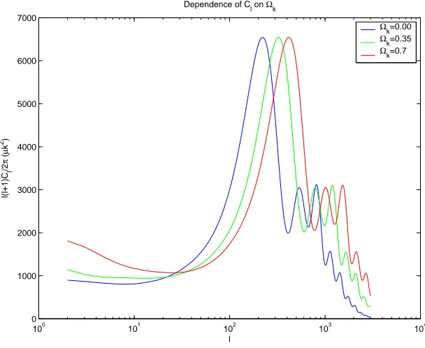
1.1 Dependence ofCℓ on Ωk, the flatness of the universe while keeping the physical matter

density fixed. . . 9

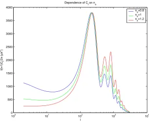
1.2 Dependence ofCℓ onns, the power law index of the primordial fluctuations. . . 10

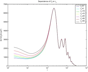
1.3 Dependence of Cℓ onτc, the optical depth in the local universe to the surface of last scattering. . . 11

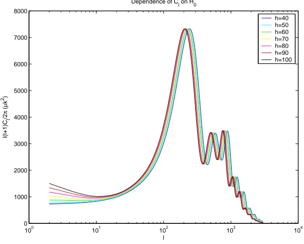
1.4 Dependence ofCℓ onH0, the Hubble constant. . . 12

1.5 Dependence ofCℓ on Ωmh2. . . 13

1.6 Dependence ofCℓ on ΩBh2. . . 13

1.7 The CBI site, which is also the future ALMA site, has been touted by many others as one of the driest, highest places in the world. The author is on the right. . . 18

1.8 The author building the CBI receivers. . . 20

3.1 Antenna configuration for the commissioning run of the CBI. . . 39

3.2 Distribution of baseline lengths during the commissioning run. . . 39

3.3 The 08 hour deep field. . . 40

3.4 The 14 hour deep field. . . 41

3.5 Phase of visibilities for a typical 1-meter baseline. . . 43

3.6 Same as Figure 3.5, but with a constant phase ramp of 1200 degrees/hour subtracted off. 44 3.7 Same data as Figure 3.5, showing the phase distribution of the differenced (ground-free) data. . . 46

(10)

3.9 The CBI fitted beam. . . 48

3.10 Comparison of CBI fit beam to the Gaussian approximation to it. . . 49

3.11 Plot showing correction factor multiplied to Rayleigh-Jeans law to get differential Black Body, dBν dT . . . 50

3.12 Power spectrum plotted in Padin et al. (2001a). . . 56

4.1 Plot of numerical estimates of the correction factor that needs to be applied to scatter-based estimates of the variance. . . 62

4.2 Comparison between spectra using a fine mesh in CBIGRIDR and a hybrid mesh with coarser sampling atℓ >800. . . 65

4.3 Relative efficiency of a two visibility experiment with one long baseline and one short baseline. . . 71

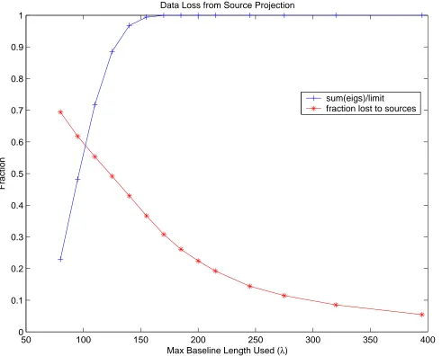
4.4 Expected behavior of total signal available and signal lost due to sources as theℓrange of the data is varied. . . 73

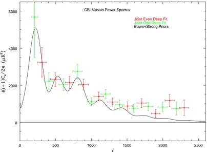
4.5 Original mosaic power spectrum using deep-field source projection parameters. . . 75

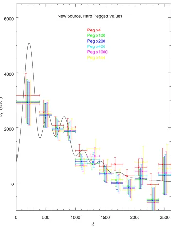
4.6 Mosaic power spectrum as a function of various source projection levels. . . 77

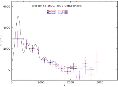
4.7 Comparison of mosaic power spectra with the data running toℓ= 2600 andℓ= 3500. 78 4.8 Map of the 02 hour mosaic. . . 80

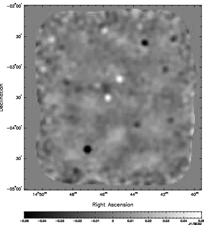
4.9 Same as Figure 4.8 for the 14 hour mosaic. . . 80

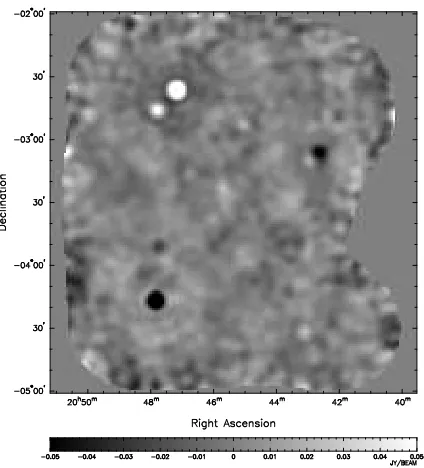
4.10 Same as Figure 4.8 for the 20 hour mosaic. . . 81

4.11 Final first-year power spectrum, binning is ∆ℓ= 200. . . 82

4.12 The CBI mosaic band power window functions. . . 83

4.13 Same as Figure 4.11, with a fit to BOOMERANG plotted for reference. . . 84

4.14 CBI spectrum, along with the BOOMERANG, DASI, and MAXIMA spectra. . . 85

4.15 Mosaic and deep field spectra, with the mosaic using the same binning as the deep. . 86

4.16 Comparison of CBI 2000+2001 data with WMAP and ACBAR. . . 87

4.17 1-D projected likelihood functions calculated for theCBI_{o140+DMR data. . . .} ₉₁

(11)

4.19 Comparison of different experiments. 2-σ likelihood contours for the weak-h prior

(ωcdm–Ωkpanel) and flat+weak-hprior for the rest, for the following CMB experiments

in combination with DMR: CBI_{e140, BOOMERANG, DASI, Maxima, and}

“prior-CMB” = BOOMERANG-NA+TOCO+Apr99 data. . . 95

5.1 Figure showing the effects of different model spectra used during compression on the higherℓCBI bin. . . 103

5.2 Same as Figure 5.1, showing the lowest-ℓbin. . . 104

5.3 Plot showing increase in bin scatters for various compression levels using a CMB spec-trum as the model for compression. . . 105

5.4 Same as 5.3 for a flat spectrum. . . 106

5.5 Same as 5.3 for a slowly rising spectrum. . . 106

5.6 Same as 5.3 for a model spectrum rising asℓ2_{. . . 107}

5.7 Equivalence of single component models with variable spectral indexαto two-component spectral index data. . . 110

5.8 Comparison of fit values between CBIGRIDR and CBISPEC, for the first bin. . . 116

5.9 Same as Figure 5.8 for the highest-ℓbin. . . 117

5.10 Figure showing the degeneracy for a single baseline between a tilt in the power spectrum (Cℓ∝ℓγ_{) and a flat power spectrum with a non-Black Body spectrum. . . 121}

5.11 Same as Figure 5.10, this time with a 125 cm baseline added. . . 122

5.12 Histogram of spectral index fits to a flat band power CMB model, made using simula-tions based on the 02 hour mosaic. . . 124

(12)

List of Tables

4.1 Band Powers and Uncertainties (from Pearson et al. (2003)) . . . 81

4.2 Parameter Grid for Likelihood Analysis. From Sievers et al. (2003) . . . 88

4.3 Cosmic Parameters for Various Priors UsingCBI_{o140+DMR. From Sievers et al. (2003) 89} 4.4 CBI Tests and Comparisons. From Sievers et al. (2003) . . . 93

4.5 Cosmological Parameters from All-Data . . . 96

5.1 Model Spectra Used in Compression Tests . . . 102

5.2 CBIGRIDR and CBISPEC Comparison . . . 115

5.3 Spectral Indices of CBI Mosaics . . . 125

(13)

Chapter 1

Introduction

About forty years ago, Arno Penzias and Robert Wilson discovered that the sky was filled with a

highly uniform glow with an antenna temperature at 4 GHz of about 3 degrees (Penzias &

Wil-son, 1965). The radiation was immediately interpreted by Dicke et al. (1965) to be the thermal

radiation from the formation of the universe that they themselves were searching for, now called

the Cosmic Microwave Background (CMB). They recognized its cosmic importance, even using the

CMB temperature and cosmic helium abundance to calculate the current physical baryon density

ΩBh2 to within an order of magnitude, using the techniques of Big Bang Nucleosynthesis (BBNS).

The CMB was measured to be an almost perfect black-body (Mather et al., 1994) and perhaps the

smoothest astronomical field known, uniform throughout the sky to a part in a thousand. Despite

its smoothness, observations of minute fluctuations in the CMB have become one of the most

impor-tant sources of information about the large-scale properties of the cosmos. This thesis will discuss

observations of CMB anisotropies using the Cosmic Background Imager (CBI), a special purpose

radio interferometer.

I will describe CBI observations, techniques used to analyze the data, and the results obtained.

In Chapter 2, I describe the framework of Maximum Likelihood Estimation used to extract a power

spectrum once the expected behavior of the data is calculated, including a new way of converging

to the best-fitting power spectrum that can decrease the computational work by a factor of a few

dozen. In Chapter 3, I describe the commissioning data taken by the CBI, the analysis techniques

(14)

describe the first-year observations of the CBI, the analysis of those data (which was much more

sophisticated than that of Chapter 3), and the ensuing power spectrum. In Chapter 5, I describe

a new, fast technique for measuring the power spectrum that has considerable flexibility in the

choice of information retained while approaching the theoretical minimum number of estimators

required to compress the data set almost losslessly. This compression is important because CMB

analysis strains available computing resources. This technique has been coded into a program called

CBISPEC, which I then use to place limits on galactic foregrounds possibly present in the CBI

observations. This is a task for which CBISPEC is well suited, but which is impossible with our

other analysis tools. In Appendix A, I carry out a derivation of statistical noise properties used in

Chapter 4. Finally, in Appendix B I briefly summarize work conducted with Patricia Udomprasert

in applying optimal CMB weighting to CBI observations of galaxy clusters. This has the potential

to substantially increase the accuracy with which the CBI can characterize cluster structure from a

given dataset.

1.1

Origin of the Microwave Background

The CMB is understood today to be the remnant radiation from the big bang. The universe started

as an extremely hot, dense plasma that expanded and cooled. This expansion and cooling has

continued from the earliest fraction of a second after the big bang through the current day. When

the universe was very young, the thermal radiation was locked in place relative to the baryons

through Thomson scattering. There was some diffusion on small scales (Silk, 1968), but otherwise

the photon density behaved like the plasma density. Finally, about 400,000 years after the big bang,

protons and electrons combined to form neutral hydrogen atoms, a process called recombination. The

photons could then free-stream, and they have been (mostly) unaltered since this epoch, aside from

the overall cooling of the CMB due to the expansion of the universe. The spot where photons last

scattered off of electrons is called the surface of last scattering. Because recombination happened

quickly (δz/z < 0.1 (see, e.g., White, 2001), we have in the CMB essentially a snapshot of the

(15)

or about the age of a day-old baby relative to a 90-year-old. At this early time, the universe was

almost perfectly uniform. But it can’t have been completely uniform, or else there would have been

no seeds from which the structure we see today could have formed. For decades, people searched for

anisotropies in the CMB without success. The first and by far the largest anisotropy measured was

a dipole moment due to the Earth’s motion, most notably in Fixsen et al. (1994) (see Lineweaver,

1997, for dipole history), but the primordial fluctuations were not detected until the COBE satellite

(Smoot et al., 1992) measured fluctuations on 10◦ _{scales in 1992. Since then, the study of the CMB}

has been one of the most active fields in astronomy, with a whole host of experiments measuring

the anisotropies with higher sensitivity and on smaller scales from ground-based, balloon-born, and

satellite experiments.

The reason that measuring CMB anisotropies is of such interest is because the angular power

spectrum of the anisotropies contains a wealth of detailed information about the properties and

evolutionary history of the universe. The power spectrum is so useful because the fluctuations

are both calculable and small. Once the earliest spectrum has been set (such as during inflation),

the evolution of the fluctuations does not depend on exotic and uncertain physics. Because the

fluctuations are small they remain in the linear regime, and so the messy non-linear physics that

dominates the universe today (star formation, gas dynamics, supernovae, AGN’setc.) doesn’t affect

the expected spectrum. Care must be taken calculating the spectrum, especially the radiative

transfer in the transition region between optically thick and optically thin. Though the calculations

are complicated, they are not uncertain, and a number of packages that calculate the spectrum are

in good agreement (Bond & Efstathiou, 1984, 1987; Vittorio & Silk, 1984, 1992; Fukugita et al.,

1990; Hu et al., 1995; Lewis et al., 2000, many others). We use versions of the fast code CMBFAST

(Seljak & Zaldarriaga, 1996) for all the model spectra used in this thesis.

1.2

Power Spectrum Basics

The primary goal of microwave background experiments is to measure the angular power spectrum

(16)

Cℓ are different quantities), so the notation used in the remainder of this work is defined here, and

power spectrum concepts specific to the CMB are outlined.

Generally, power spectra are thought of in Fourier space, as being the expected variance of

modes of a given wavelength. The fact that the sky is a sphere, rather than an infinite plane,

requires modifications to the standard Fourier picture. For the particular case of the surface of

a sphere, the temperature everywhere on the sky is expressed as the sum of spherical harmonics,

rather than the sine and cosine waves of Fourier transforms:

∆T

T =

X

ℓ ℓ

X

m=−ℓ

aℓmΦℓm(θ, φ) (1.1)

Here the Φℓmare the spherical harmonics, and theaℓmare their amplitudes. With the Φℓm,ℓmore

or less corresponds to the wavelength of the mode, andmis akin to its orientation. Since we expect

the microwave background to have no preferred orientation on the sky, theaℓmshould be statistically

independent ofm, depending only onℓ. Furthermore, we expect the CMB to be a Gaussian random

field if the fluctuations arise during the era of inflation (White, Scott, & Silk, 1994), though other

sources of structure formation,e.g.topological defects, will give rise to non-Gaussianity. This means

that theaℓmare independent of each other and have a Gaussian probability distribution with mean

zero. Under these assumptions,all of the information contained in the CMB is contained in a set

of coefficients Cℓsuch that

a2ℓm

= Cℓ (1.2)

This is not usually the quantity quoted, however. To see the problem, picture a power spectrum

where Cℓ is constant and compare the variance on small scales to that on large scales. If we pick

a patch size of interest, then it will feel power from some fractional width inℓ, so a small patch at

higherℓ will feel more discrete values of ℓ than a large patch at lower ℓ. In addition, each ℓ feels

2ℓ+ 1 individual Φℓm, and so the total number ofaℓm that contribute to the variance of a patch is

proportional toℓ2_{. So, a flat power spectrum in C}

ℓ will have sharply rising temperature fluctuations

(17)

spectrum with every mode statistically equivalent, so large-scale fluctuations average over more noise

and hence will have smaller amplitudes than small-scale fluctuations. In order to make the numbers

in the power spectrum more physically meaningful, the quantityCℓis often used, with the definition

(Bond, 1996)

Cℓ≡ ℓ(ℓ+ 1)C_2π ℓ (1.3)

A flat spectrum inCℓ will then have scale-invariant temperature fluctuations, equal on all lengths.

Usually,Cℓis scaled by the CMB temperatureT0and plotted inµK2. This corresponds to the actual

temperature variance on the sky of fluctuations with wavenumberℓ. In general, the remainder of

this work will refer toCℓand not Cℓ.

1.3

Cosmological Effects on the Power Spectrum

The initial fluctuations are believed to have arisen from quantum uncertainty during the epoch

of inflation, and hence to have a nearly scale-invariant spectrum, though the details depend on

which particular flavor of inflation one uses (see, e.g., Lyth & Riotto, 1999, for a review). Since

the creation of the fluctuations, there are two broad classes of effects that determine the present

day power spectrum—those processes that happened before recombination and those that happened

after. The post-recombination effects include scattering off the reionized electrons in the modern

universe (seen in Kogut et al., 2003), anisotropies introduced because of the time-varying potential

along the flight path of a photon called the integrated Sachs-Wolfe effect, an overall size scaling

in ℓ of the power spectrum set by the angular diameter distance to the surface of last scattering,

and heating of CMB photons on small scales due to Compton scattering off hot gas in clusters,

called the Sunyaev-Zeldovich effect. Before recombination, the photons were locked in place with

the baryons, and so they carry the information about the state of the baryons at 400,000 years. The

baryon/photon fluid underwent acoustic oscillations as overdense regions collapsed due to gravity,

then expanded from pressure, while the dark matter continued to collapse. Because the fluctuations

(18)

a short period of time at the surface of last scattering, the phase of fluctuations at the surface of last

scattering is only dependent on their wavelengths. So we expect to see the power rising as we go to

smaller scales up until the length where the fluctuations are at their maximal compression (atℓ∼200

for a flat universe). As we move to smaller scales, the power will drop as the scale length moves

towards modes that have completed their first compression and are expanding back to a density null

(but a peak in the velocity). Then we will see modes that have compressed, re-expanded, and hit

the point of maximal expansion, for another peak in the power spectrum. And so on down to ever

smaller scales that have completed more and more oscillations by the surface of last scattering. So,

we expect to see peaks and dips in the angular power spectrum of the CMB. The details are very

sensitive to the exact conditions of the universe, though. Dark matter has no pressure, and so rather

than oscillate it will continue to collapse, and try to pull the photon-baryon fluid with it through

gravity. On small scales, photons will diffuse out of the fluctuations, reducing power exponentially

in a process called Silk damping (Silk, 1968). On larger scales, photons are gravitationally redshifted

by climbing out of the potential wells of the perturbations, called the (non-integrated) Sachs-Wolfe

effect (Sachs & Wolfe, 1967). The effect is 1/3 that expected solely due to gravitational redshifting

because time dilation at the surface of last scattering partially cancels the gravitational redshift,

since it causes the photons to appear to come from a younger, hotter universe (c.f.Peacock, 1999).

As the fluid collapses, the more baryons there are driving the infall, the more pressure the photons

have to exert before they can turn the collapse around, leading to an increase in power in the odd

numbered (compression) peaks. Power on small scales is also reduced because of the finite thickness

of the surface of last scattering. Instead of seeing a single fluctuation, as is the case for large-scale

modes, a single point on the sky will have contributions from the number of small modes that can

fit into the finite recombination thickness. Consequently, the average temperature anisotropy drops

from purely geometric effects on small scales (in addition to the reduction from Silk damping). This

can be used to test, e.g., non-standard recombination theories (for instance, if the fine-structure

constantαvaries with time). Because the amplitude at the surface of last scattering is proportional

(19)

primordial fluctuations in the microwave background. It is precisely because the evolution of the

fluctuations is sensitive to so many fundamental parameters that detailed observations of the CMB

fluctuations can determine many fundamental parameters.

I have found a few simple rules helpful when trying to understand the behavior of the power

spectrum that will be illustrated in Figures 1.1 through 1.6, which plot sample power spectra. All

spectra were calculated using CMBFAST. The unit of density used in cosmology is Ω, which is the

fractional density of a component relative to the critical density required to make the universe flat.

For matter densities, this is not the important density. Rather, the important density is the physical

density at the surface of last scattering, which (absent the creation or destruction of particles) is

the same as the physical density today, scaled by the relative volumes of the universe, (1 +z)3_.

Because the critical density depends on the Hubble constant likeH0−2, a fixed physical density will

be proportional toH2

0Ω. In keeping with astronomical tradition, the Hubble constant will be listed

as 100hkm/s/Mpc. So, the physical density of the component of the universe x will be given as

Ωxh2, which is sometimes also written in the literature as ωx. For these figures, unless explicitly

varied, the baryon physical density ΩBh2, the cold dark matter density Ωcdmh2, and the total matter

density Ωmh2≡ΩBh2+ Ωcdmh2 will be kept fixed, unless explicitly varied. The other cosmological

parameters that specify the models are the spatial curvature of the universe Ωk, the scalar power-law

index of the primordial fluctuationsns, the cosmological constant ΩΛ, and the optical depth due to

reionizationτc. The Hubble constant is implicitly defined through the relation Ωk+ ΩΛ+ Ωm= 1.

The fiducial model in the plots is Ωk = 0 (flat universe), h = 69, ΩBh2 = 0.023, Ωmh2=0.143,

ΩΛ= 0.699,ns= 1.0, andτc = 0, with one parameter varied in each set. When Ωk, ΩBh2, Ωmh2,

and h were varied, ΩΛ was varied to maintain Ωk + ΩΛ+ Ωm = 1. Rather than the traditional

normalization to COBE-DMR at low-ℓ, I normalize the plots to the value at the first peak. This is

often more illustrative than the traditional normalization, for instance, in theCℓas a function ofh

plot.

There is a distinction between the power spectrum at the surface of last scattering and the

(20)

at a given redshift, it cannot be coherent on scales larger than the horizon size at that redshift,

so we expect the signature of events between the surface of last scattering and the present day to

be primarily concentrated at low-ℓ, while the fluctuations intrinsic to the surface of last scattering

to appear predominantly at high-ℓ. One such effect is from the reionization of the universe by

stars at a comparatively recent redshift. When reionization happens, CMB photons will scatter

off the newly free electrons. Since the scattering happens through large angles, it essentially leads

to an average scattered component equal to the mean CMB temperature as seen by the scattering

electron. That scattering will average out over scales smaller than the electron’s horizon size, but

not over larger scales. Since the electron density after reionization will fall like (1 +z)3, most of the

scattering will happen near the redshift of reionization, so the effect on the spectrum will be roughly

to reduce the amplitude on scales smaller than the horizon by exp(−τ) while leaving the larger scales

mostly untouched. This is indeed the case, as can be seen in Figure 1.3. Another important large-ℓ

secondary anisotropy is the integrated Sachs-Wolfe effect, which is the heating or cooling of photons

as they travel through a changing gravitational potential. If a potential weakens as a photon travels

through it (e.g., from a matter overdensity expanding with the Hubble flow), then the blueshift as

the photons falls into the potential well will be larger than the redshift as the photon climbs out.

This is the one place that the cosmological constant Λ can effect the CMB spectrum (other than

an its effect on Ωk, which doesn’t change the shape of the spectrum), since larger values of Λ in

a flat universe mean that the expansion is Λ-dominated earlier, and so the integrated Sachs-Wolfe

contribution to the spectrum is larger in amplitude and happens on smaller scales. This effect is

clearly seen in Figure 1.4, which keeps Ωk and the physical matter densities ΩBh2 and Ωmh2 fixed

while trading betweenhand Λ. Ashincreases, ΩB and Ωm decrease to keep the physical densities

fixed, leading to a higher value of Λ to keep the universe flat. This shows up at very low-ℓ(about

(21)

100 101 102 103 104 0

1000 2000 3000 4000 5000 6000 7000

l

l(l+1)C

l

/2

π

(

µ

k

2)

Dependence of C l on Ωk

[image:21.612.172.476.204.453.2]

Ω_k=0.00 Ω_k=0.35 Ω_k=0.7

Figure 1.1 Dependence of Cℓ on Ωk, the flatness of the universe while keeping the physical matter

density fixed. The curvature of the universe doesn’t affect the physical structure at the surface of last scattering, since the universe was highly matter+radiation dominated then. It can only affect the angular diameter distanceDA to the surface of last scattering, so the acoustic peaks are

shifted to largerℓas the universe become less dense, without changing the structure of the peaks. Conveniently, DA is sensitive predominantly to the overall spatial curvature of the universe, and

only weakly sensitive to which individual constituents dominate. This is why the position of the first peak, which is really a direct measure of DA, is so useful as a measure of the flatness of the

(22)

100 101 102 103 104 0

500 1000 1500 2000 2500 3000 3500 4000

l

l(l+1)C

l

/2

π

(

µ

k

2)

Dependence of C_l on n_s

[image:22.612.172.477.75.325.2]

n_s=0.8 n_s=1 n_s=1.2

Figure 1.2 Dependence ofCℓ onns, the power law index of the primordial fluctuations. Inflationary

theories predict a value slightly less than one. Measurement over very broadℓranges increases the sensitivity tons. There has been a recent suggestion (Spergel et al., 2003) that the initial spectrum

may have been more complicated than a simple power law.

1.4

Microwave Background Observations

The first detection of anisotropy in the CMB was that of the Differential Microwave Radiometer

(DRM) on COBE (Smoot et al., 1992), which measured the power spectrum on scales of∼10◦_{. Ever}

since, there has been a flurry of activity in the field. The first generation of post-COBE experiments

(e.g.Bond et al. (2000) for a list) concentrated on measuring the first acoustic peak, which for a flat

universe is on angular scales of about a degree, orℓ∼200. Many experiments dectected anisotropies,

but no single experiment succeeded in convincingly detecting a peak internally, though TOCO (Miller

et al., 1999) came tantalizingly close. The combined set of experiments suggested the presence of

a peak, but the heterogeneous nature of the data and the comparatively large errors of any single

data set made the peak in the ensemble set somewhat questionable. The field changed dramatically

with the first unambiguous detection of an acoustic peak by BOOMERANG (de Bernardis et al.,

(23)

100 101 102 103 104 0

1000 2000 3000 4000 5000 6000 7000

l

l(l+1)C

l

/2

π

(

µ

k

2)

Dependence of C l on τc

[image:23.612.172.478.208.459.2]

τ_c=0 τ_c=5 τ_c=10 τ_c=15 τ_c=20 τ_c=30 τ_c=40

Figure 1.3 Dependence of Cℓ on τc, the optical depth in the local universe to the surface of last

scattering. The assumption is that the universe reionized quickly at a given redshift and has remained largely ionized ever since. The CMB gets averaged out on scales smaller than apparent horizon size at recombination, but is largely untouched on larger scales. So, reionization picks out a special ℓ, and fluctuations smaller than thatℓare suppressed relative to fluctuations larger than thatℓ. Since the plot is normalized so that the models are equal to each other at their peaks, this shows up as an amplification of power at smallℓatτc increases. The higherτcis, the earlier the universe must have

(24)

100 101 102 103 104 0

1000 2000 3000 4000 5000 6000 7000 8000

l

l(l+1)C

l

/2

π

(

µ

k

2)

Dependence of C_l on H₀

[image:24.612.170.479.205.453.2]

h=40 h=50 h=60 h=70 h=80 h=90 h=100

Figure 1.4 Dependence of Cℓ onH0, the Hubble constant. This is an example of a degeneracy in

the microwave background. If we keep the physical densities of matter components ΩBh2and Ωmh2

fixed as we varyH0, then the physical densities at recombination will also remain unchanged. This

plot keeps ΩBh2 and Ωmh2 fixed, changing Λ to keep the universe flat for different values of H0.

The slight horizontal shifting for the different models is due to the degree to which DA is sensitive

to the constituents of the universe rather than just to its flatness. It is precisely this degeneracy between H0 and DA that makes the CMB, by itself, unable to measure Λ. There is a difference

at low-ℓbecause the Sachs-Wolfe effect is changed by the different expansion history, but it can be mimicked by other factors such asτc. The intrinsic cosmic variance on such large scalesℓ∼10 also

(25)

100 101 102 103 104 0 1000 2000 3000 4000 5000 6000 7000 8000 9000 10000 l l(l+1)C l /2 π ( µ k 2)

Dependence of C l on ωm

ω_m=0.05 ω_m=0.10 ω_m=0.15 ω_m=0.20 ω_m=0.25 ω_m=flat

Figure 1.5 Dependence ofCℓ on Ωmh2. Same as Figure 1.1, only varying the dark matter content

while keeping the universe flat andhfixed.

0 500 1000 1500 2000 2500 3000

0 1000 2000 3000 4000 5000 6000 7000 8000 9000 l l(l+1)C l /2 π ( µ k 2)

Dependence of C_l on ω_B

ω_B=0.005 ω_B=0.011 ω_B=0.017 ω_B=0.023 ω_B=0.031 ω_B=0.040

Figure 1.6 Dependence of Cℓ on ΩBh2. This figure has been plotted on a linear scale without

normalization to make the behavior in the second and third peaks easier to see. Note how the second peak amplitude drops and the third peak rises as ΩBh2 increases. Also note that power is

suppressed at higherℓby low values of ΩBh2 because photons diffuse faster with fewer baryons to

(26)

predicted to be if the universe were flat. In addition to measuring the first peak, BOOMERANG

and MAXIMA probed smaller angular scales as well, beginning to unlock the information contained

in the spectrum at higherℓ. The BOOMERANG and MAXIMA spectra were joined in short order

by spectra from CBI (Padin et al., 2001a; Mason et al., 2003; Pearson et al., 2003), DASI (Halverson

et al., 2002), VSA (Scott et al., 2003; Grainge et al., 2003), ARCHEOPS (Benoˆıt et al., 2003),

and ACBAR (Runyan et al., 2003), as well as improved spectra from BOOMERANG (Netterfield

et al., 2002; Ruhl et al., 2002) and MAXIMA (Lee et al., 2001). Of note are the first detection

of the damping tail by CBI (Padin et al., 2001a), the first detection of the polarization signal of

the CMB by DASI (Kovac et al., 2002), and a possible first detection of secondary anisotropy from

the Sunyaev-Zeldovich effect by the CBI (Mason et al., 2003; Bond et al., 2002b), later joined

on the same angular scales by BIMA (Dawson et al., 2002) and ACBAR. This second generation

of ground-based or balloon-born experiments has been characterized by high signal-to-noise ratio

(SNR) measurements of the CMB spectrum over large ranges of angular scales. This permits single

experiments to trace out important structures in the power spectrum. In addition, the different

power spectra are in good agreement (see,e.g., Sievers et al., 2003), which gives one confidence in

them. This second generation is being brought to completion by the WMAP satellite and its all-sky

power spectrum (Hinshaw et al., 2003), which is very good toℓ∼600 and cosmic-variance limited

to ℓ∼350. It is worth stressing that where WMAP is cosmic variance limited, it has used all the

information present in the full sky. No future experiment will be able to substantially improve the

total-intensity spectrum through the first peak.

There will be two main thrusts in future microwave background observations. The first is to do

an ever better job of measuring the power spectrum on smaller scales. There will be an improvement

through the second and third peak region of the spectrum as WMAP continues observing. Upcoming

experiments, such as Planck, the Atacama Cosmology Telescope, and the South Pole Telescope, will

also improve the spectrum out to higherℓ, with the hope of eventually finding galaxy clusters because

of their imprint on the CMB through the Sunyaev-Zeldovich effect (see, e.g., Komatsu & Seljak,

(27)

polarization of the microwave background. DASI (Kovac et al., 2002) first measured the polarization

power spectrum, though the spectrum is too noisy to have cosmologically useful information. Shortly

thereafter, WMAP measured the cross-correlation spectrum of the polarization and total-intensity

anisotropies on large scales (Kogut et al., 2003). This large-angle spectrum contains information

about the optical depth to the surface of last scattering. The optical depth comes from free electrons

after hydrogen has been ionized by the first sources of light in the universe. Because the scattering

from electrons is polarized, and the radiation scattered is the CMB as seen by the scattering electrons,

τc introduces a correlation between the total intensity and the polarization of the CMB. It is this

that allowed WMAP to break the degeneracies in total intensity to measure τc and find that the

universe reionized atz= 20±10. Future measurements will refine this number.

1.5

Interferometers

I give here a brief description of interferometers, along with some of the terminology used throughout

this thesis. For more quantitative details as to the response of interferometers, especially with regards

to CMB observations, see Chapter 3. Radio frequency interferometers are an important part of

microwave background research. The CBI, along with DASI and the VSA, are radio interferometers.

The remaining second-generation ground/balloon based CMB experiments use bolometers to map

the total intensity of the CMB in maps. An interferometer consists of an array of collection devices

(usually parabolic dishes, but sometimes feed horns as is the case with DASI and VSA), with a

receiver at the focus of each dish sensitive to the incoming electric field. The receiver amplifies

the electric field, then usually the signal is mixed down to lower frequencies and perhaps split into

channels. The receiver outputs are then fed into the correlator which multiplies the signals from

each pair of receivers and integrates the product. The fundamental measurement produced by an

interferometer is this integrated signal product, called avisibility. Because incoming electric fields

have amplitudes and phases, the visibilities need amplitudes and phases as well, which makes them

complex, so each visibility really has two independent pieces of information. Thebaseline is the pair

(28)

the antenna pair, or more commonly, using the separation vector of the dishes either in physical

distance or in wavelengths. The vector position of the baseline in wavelength is known as the UV

position of the visibility, and the total set of UV points observed by an interferometer is called the

UV coverage. The areas in the UV plane covered by observations sets the total range of scales to

which the interferometer is sensitive. The noise, usually dominated by thermal noise in the receivers,

is independent for different visibilities. There can be correlated noise between different visibilities,

but in a well-designed instrument it should be very small, with the receiver cross-talk in the range

of -110 to -130 dB for the CBI’s most closely-spaced dishes (Padin et al., 2000).

The response of a visibility to the signal on the sky depends both on the separation of the

dishes and the details of the collecting element. Perhaps the easiest way to visualize the output

of an interferometer is to run the signal backwards and think of the receiver as a transmitter.

For the case of a single dish, there will be a single-aperture diffraction pattern on the sky that

is the Fourier transform of the collecting aperture. The power pattern on the sky is called the

primary beam and is the Fourier transform of the square of the electric field response of the dish.

It typically has a large response in the center, with ripples extending out to large angles falling in

amplitude. The surrounding ripples are called sidelobes. Sidelobes are undesirable because they

make the interferometer respond to (usually unknown and possibly changing) sources far away from

the position on the sky where the dish is pointed, called the pointing center. Consequently, there

is often some sort of taper applied to the dish to make the sidelobes fall off more quickly, at the

expense of a slight broadening of the main part of the beam and a reduction in sensitivity. In

the CBI dishes, we use a Gaussian taper since the reduction in sidelobes is so important. For the

case of a two-element baseline, a phase modulation gets applied to the primary beam because the

radiation from the two receivers alternately goes in and out of phase, with the wavevectorkof the

visibility on the sky equal to the vector separation of the baseline in wavelengths, which is theU V

coordinate of the baseline. Note that each element is sensitive to the electric field, so the product

of two baselines will be sensitive to the square of the electric field, which is precisely the single dish

(29)

the receivers again, a visibility will be equal to the integral of primary beam times a plane wave

on the sky times the sky signal. In Fourier space, the multiplication becomes a convolution, and

we have that the visibility is equal to the Fourier transform of the sky convolved with the Fourier

transform of the primary beam, sampled at the UV coordinate of the baseline (see Chapter 3 for

quantitative details of the response). It is precisely this property that makes interferometers well

suited for CMB observations: on small scales, the power spectrum Cℓ is equivalent to the Fourier

space power spectrum, which is exactly what an interferometer measures, modulo the smearing by

the primary beam. Unlike the bolometer experiments where each pixel sample the entire range ofℓ

up to the pixel size, interferometer data are localized inℓ. Other advantages of interferometers are

ease of measurement of the primary beam (notoriously difficult for balloon-born bolometers), stable

calibration, and well-behaved noise properties since the visibilities have independent noises.

1.6

The Cosmic Background Imager

The Cosmic Background Imager (Padin et al., 2002) is a special purpose interferometer located in

the Atacama desert of northern Chile. The site is both high and dry, making it an excellent place

for centimeter-wavelength observations (though a non-negligible fraction of the time has been lost

due to weather. See Figure 1.7). The CBI has 13 low-noise HEMT receivers, with a total system

temperature of about 30 Kelvin, co-mounted on a 5.5 m rotating deck. The receivers accept a single

circular polarization. During the observations described here, 12 receivers were set to measure left

circular polarization, with the thirteenth receiver set to right circular polarization, in order to retain

some polarization sensitivity. The polarization results are described elsewhere (Cartwright, 2002).

The signals are downconverted and split into 10 1GHz channels between 1 and 2 GHz that are then

combined using a high-speed analog correlator (Padin et al., 2001b). Rather than be locked into

a single observing pattern, the dishes can be moved around the telescope mount in order to give

the CBI maximum flexibility in its UV coverage. Each of the 10 channels per baseline is recorded

separately, and since the fractional bandwidth is wide (R∼3), each baseline covers a fractional width

(30)

(31)

tangentially without having to wait for the Earth to do the rotation for us. As a consequence, we

have very dense UV coverage (see Figure 3.1 for a sample of the CBI UV coverage). The deck can

be tilted to an angle of 42.75 degrees above the horizon, limiting the CBI observations to roughly

−70 < δ < +24, and limiting the length of time a single source can be tracked to < 6.5 hours,

depending on the declination.

Prior to shipping the CBI to Chile, we assembled and tested it on the Caltech campus in

Pasadena. The initial construction period was from early 1998 to August 1999. I worked on the CBI

at that time, assembling and testing the receivers (see Figure 1.8). The construction was completed

sufficiently for first light in Pasadena in January 1999, using three receivers. During the testing in

Pasadena, we found that the CBI worked well, but that ground spillover in the sidelobes of the small

dishes was substantial (see Section 3.2 for further discussion). After several months of testing, we

disassembled the CBI and shipped it to Chile in August of 1999. Once there, it was transported to

the site and reassembled, with first light on-site in December 1999. The first science observations

of the microwave background were taken January 12 of 2000, and, apart from maintenance, repairs,

and upgrades, the CBI has been taking data ever since (weather permitting). The first two years

were devoted to total intensity measurements of the power spectrum, with the CBI switching in the

(32)

(33)

Chapter 2

Maximum Likelihood

Our task is to measure Cℓas accurately as we can. The conceptually simplest case is that of an all-sky

map with no noise or contaminating signals, such as point sources or diffuse galactic foregrounds. In

that case we could simply decompose the sky into its constituent modes and measure their variances.

A real experiment is complicated by partial sky coverage (which can introduce apparent correlations

between the aℓm), noise, point sources, galactic foregrounds,etc. But at its heart, CMB analysis is

still nothing more complicated than measuring the variance of a data set.

2.1

Uncorrelated Likelihood

We can better understand how to measure the power spectrum by starting with the simple case of

a single Gaussian random variable and then adding more and more complexity to the problem. For

a single Gaussian random variablexwith zero mean and varianceV =σ2_{, the PDF is}

P DF(x) = exp(−

x2

2V) √

2πV (2.1)

This is the probability density that we would get a certain value forxgiven the underlying variance.

This can also be thought of as the likelihood that we would have gotten the observed data pointxif

the underlying variance wereV. This interpretation gives rise to the method of Maximum Likelihood

estimation of the variance. Our estimated value ofV is that which would have yielded the observed

(34)

P(V|x) = P(x|V). This is equivalent to the standard Bayesian expressionP(V|x) =P(x|V)P(V)

with a uniform prior on V, i.e., all values of V are equally probable by assumption. While not

important for maximum likelihood estimation, this does show how in principle we could include

prior knowledge of likely power spectrum or cosmological parameter values.

For the case of a single value, the maximum likelihood estimator for the variance is set by

maximizing the likelihood with respect toV. We usually work with the log of the likelihood rather

than the likelihood itself, as the log likelihood is mathematically simpler to use.

log (L) =−1

2 x2

V −

1

2log 2πV (2.2)

The derivative is

dlog (L)

dV =

1 2

x2

V2 −

1

2V (2.3)

If we set that equal to zero and solve for V, we find the standard resultV =x2 _{– our estimate}

of the variance is equal to the actual variance of the data point. The extension to many

indepen-dent, identically distributed data points is straightforward. Because they are indepenindepen-dent, the joint

likelihood is merely the product of the individual likelihoods. In log likelihood space, the joint log

likelihood is the sum of the individual likelihoods. We typically ignore the additive constants to the

log likelihood since they don’t affect the position of the peak or the shape of the likelihood surface

around that peak. The log likelihood is then

log (L) =−1₂ n X i=1 x2 i

V −log(V)

(2.4)

We can again maximize with respect toV to get

dlog (L)

dV = 1 2V2 n X i=1 (x2

i −V) = 0 (2.5)

Again, this has a familiar solutionV =P x2

i/n=

−

x2

i, our estimate of the variance is just the average

(35)

from inside the sum

dlog (L)

dV = 1 2V n X i=1 _x2 i

V −1

= 0 (2.6)

Note that the definition χ2

i is x2i/V, hence the maximum of the likelihood is the point where the

average value ofχ2_{is equal to one.}

Real data usually have many contributions to their variance (signal, noise...), of which we may

only be interested in fitting for a single one. Also, each data point can have a different expected

response under a certain model. If we have a simple experiment that takes uncorrelated noisy data,

then the expected variance of a data point isVi=qSi+Ni, whereNiis the (Gaussian) variance due

to noise of theith_{data point,}_q_{is an overall amplitude we wish to measure, and}_S

iis the response of

theith_{data point to a unit amplitude}_{q. In principle, we could have a more sophisticated dependence}

on the parameterqwhich would complicate derivatives, but in practice that is a sufficiently flexible

model for the CMB variance. In this case, we wish to maximize the likelihood as we varyq

log (L) =X−1₂ x

2

i

qSi+Ni −

1

2log(qSi+Ni) (2.7)

dlog (L)

dq =

X1 2

x2

i

(qSi+Ni)2

Si−

1 2(qSi+Ni)

Si= 0 (2.8)

This has a solution where

X qS_i

qSi+Ni

_x2

i

qSi+Ni −

1

= 0 (2.9)

(with an extra factor of q multiplied on both sides). We are still setting the average value of χ2

equal to one, but this time subject to a set of weights. Note that the total signal variance (or square

of the signal amplitude) isqSi, so theithweight is _SignalSignal₊_{N oise}. So, the condition at the maximum

is

X qS

qS+N χ

2

−1

= 0 (2.10)

Note that as we change our model (by changing q), in addition to χ2 _{changing, the weights also}

(36)

signals and asymptotically approaches one for signals much larger than the noise. This means that

once we have reasonably well determined a data point, a better measurement of that point does not

significantly improve our estimate ofq— we are better served by measuring more data points. This

is known as the cosmic variance limit, and is the reason why CMB experiments try to cover as much

sky as possible (morexi’s). The extension to many signal components is straightforward—maximum

likelihood continues to try to set the weighted values ofχ2 _{equal to one.}

2.2

Correlated Power Spectrum

Experimental data are typically correlated, and so the simple techniques of the preceding section are

not directly applicable to real life situations. Fortunately, they can be extended to correlated data.

First, note that the log likelihood for uncorrelated data can be written as a set of matrix operations

log (L) =−1₂xTΛ−1x₋1

2log(|Λ|) (2.11)

with Λ the diagonal matrix whose elements Λiiare simply the variances of thexi. (A quick work on

notation: In general in this thesis, bold quantities are vectors, capitalized Roman letters are

matri-ces (or single elements of matrimatri-ces if subscripted), and other quantities are italicized in equations.)

Noting that the determinant of a diagonal matrix is the product of the diagonal elements, and the

inverse of a diagonal matrix is the same matrix with the elements along the diagonal inverted, the

in-dividual multiplications, divisions, etc., we carry out are identical for both the standard uncorrelated

data representation and the matrix representation of the likelihood. We can then use machinery of

matrix mathematics to transform the case of uncorrelated data into a realistic, correlated problem.

To proceed, introduce an orthogonal matrix V (distinct from the uncorrelated variable varianceV,

to which we no longer refer). An orthogonal matrix has the propery that theith_{column dotted with}

the jth _{column is} _δ

i,j – in other words, its transpose is its inverse. It is also true in general that

the determinant of the product of two matrices is the product of their individual determinants, and

(37)

have

|VTV|=|I|= 1−→ |V|2= 1 (2.12)

We can transform the uncorrelated likelihood using this matrix V while leaving the likelihood

un-changed.

log (L) =−1₂xTΛ−1x₋1

2log(|Λ|) =− 1 2x

T_VVT_Λ−1_VVT_x

−1₂log(|VTΛV|) (2.13)

The likelihood is identically unchanged because inserting VVT _{is simply multiplying by unity, and}

the determinant is multiplied by|V|2_{, which we have already shown to be one as well. We can now}

group terms using the definitions∆_≡VT_x_{and C}_≡_VT_{ΛV. The likelihood then becomes}

log (L) =−1₂∆TC−1∆₋1

2log(|C|) (2.14)

This is the standard expression for the likelihood of a theory under a particular data set that starts

off most microwave background analysis papers. The meaning of V and Λ are now clear: they are

the matrix of eigenvectors and their corresponding eigenvalues of the matrix C. Unfortunately, in

general we cannot work in the diagonal space because as we change the theory, both the eigenvectors

and eigenvalues change, and so a fixed transform does not remain diagonal. We need one more result

before this becomes practically useful, namely, how do we compute C?

First, let us find the covariance of two data points. Using the definition of∆, we have

∆i=

X

Vi,jxj (2.15)

and the expectation of the product of two∆i’s is

h∆i∆ji=

DX Vi,kxk

X Vj,lxl

E

(38)

Since the xi are independent, any term with k not equal tol has an expected value of zero. Also

note that

x2_i

= Λi, leaving

h∆i∆ji=

X

Vi,kVj,kΛk (2.17)

Now, what are the components of the transformed matrix C? Multiplying V on the left by Λ

multiplies the rows of V by the corresponding element of Λ

Vi,k →Λk (2.18)

We get the final answer for the element of C by multiplying by the inital VT_{. The}_{i, j}th_element

of the product of two matrices is the ith_{row of the first times the} _jth_{column of the second. Since}

the first matrix is the transpose of V, the ith _{row of V}T _{is the}_ith _{column of V. So, we have the}

following expression for the elements of C

Ci,j=

X

Vi,kVj,kΛk (2.19)

But this is exactly the expectation value from Equation 2.17! So, in order to calculate the

likelihood of a theory, we need only calculate the expected covariance of pairs of data points under

that theory, and then calculate the likelihood using Equation 2.14. It is because the matrix C is

made up of the data covariances that is is known as thecovariance matrix. Because∆i∆j =∆j∆i,

the covariance matrix is symmetric. The problem of measuring the power spectrum then falls into

two fairly distinct parts: The first is calculating C for our data set ∆ for different theories, the

second is how to efficiently find the theory that maximizes the likelihood, as well as characterizing

the likelihood surface around that peak. Because typical data sets can have upwards of hundreds

of thousands of data points, and calculating the likelihood is an order n3 _{operation, considerable}

care is required in both parts to make the problem computationally feasible. For instance, the CBI

(39)

then take of order (8×105)3/2×109∼10 years to invert the matrix, and would require∼5 terabytes

of memory to store it! Clearly, great care must be taken when creating C to make it as small as

possible, and then one must work with it as efficiently as possible.

2.3

Likelihood Gradient

It is now time to find the Maximum Likelihood spectrum. One often sees the likelihood that a given

spectrum would give rise to an observedcomplex data set written as (e.g.White et al., 1999)

L(Cℓ) = 1

πn_|_C_|exp

−∆†C−1∆ (2.20)

The missing factors of two relative to Equation 2.14 are because each visibility is really two

inde-pendent points, one real and one imaginary, combined. The rest of this section will use the form of

Equation 2.14 with the understanding that all complex measurements have been split into two real

data.

Our task is to varyCℓ, which changes the covariance matrix C, until we have reached the

maxi-mum of the likelihood. We restrict ourselves to models of the form

C =X

B

qBWB+ N (2.21)

where N is our generalized noise matrix (it could have contributions from thermal noise, correlated

noise between visibilities, galactic foregrounds, point sources, ground pickupetc. ), the qB are the

band powers describing the CMB power spectrum, and the WB describe the response of the data

to those band powers, equivalent to _dqdC

B. We will sometimes refer to the WB as window matrices

(since they are the matrices consisting of the visibility window functions, discussed in Section 3.3 and

elsewhere). By restricting ourselves to this form, we can again use the technique of Section 2.2 where

we calculate the gradient in the case of uncorrelated data and then transform it to the correlated

(40)

the multidimensional search method used is relatively efficient, simply varying theqB is not a bad

way of reaching the peak, and in fact is what we use in Chapter 3. Because to measure the likelihood

we need only factor C into the triangular matrix L such that LLT = C (a Cholesky factorization.

See below for how to obtain the likelihood), a single calculation of the likelihood can be very much

faster than iterations of more sophisticated methods that converge in fewer steps. For instance,

using the LAPACK linear algebra library (Anderson et al., 1999) on a Pentium IV, factoring C is

about six times faster than inverting it. To see how to get the likelihood from factoring, note that

what we really need is C−1_∆ _{and log}_|_C_|_{. To get the determinant, we need merely multiply the}

diagonal elements of L, and to get C−1_∆_{, we solve the system of equations C}_y₌_∆_{which is done}

inO n2

time once C is factored.

We can do better than that, though, especially if we are fitting many bins. If we could characterize

the likelihood surface around a point, in addition to being able to converge to the maximum more

quickly (through, for instance, Newton-Raphson iteration), we could also directly estimate quantities

of interest such as errors. Many authors have advocated calculating or approximating the gradient

and curvature of the likelihood (Bond et al., 1998; Borrill, 1999e.g.), then using Newton-Raphson

iteration to find the zero of the gradient. In order to do this, we need to be able to calculate gradients

and curvatures of the likelihood. I show here the calculation of the gradient, with the curvature

discussed in Section 2.4.

Recall the formula for the derivative of the likelihood of uncorrelated data under these

assump-tions, Equation 2.8. First let us analyze the second term, originating from the log of the determinant

of C

−X 1

2(qSi+Ni)

Si (2.22)

The denominator is the total variance Λ−1_i (inverse since it’s in the denominator), while the coefficient

is the change in Λiwith respect to the parameter in questionq. So, we would like a matrix operation

that will multiply those two sets of numbers and sum them. Fortunately there is such an operation—

(41)

property that it is the sum of the eigenvalues, and hence is unchanged when we rotate the matrix.

So, we can write the term as follows

−X_2(qS1

i+Ni)

Si=−

1 2

XΛi,q

Λi

=−1₂T r Λ,qΛ−1

(2.23)

where Λ,q is the derivative of Λ with respect to the band powerq. We can now rotate from Λ to C

since the trace is unaffected, giving the general expression

−1

2T r C,qC

−1

(2.24)

The first term, which is theχ2 _{of the data}

X1 2

x2

i

(qSi+Ni)2

Si (2.25)

is rather more interesting since there aretwoways it can be transformed into matrix notation, both

of which are useful. It is reasonably straightforward to process it in the diagonal case and then

rotate, but is not trivial because some care must be taken when rotating multiple matrices that

do not have the same eigenvectors. Instead, I will proceed directly from the matrix description

−1 2∆

T_C−1_∆_{. We will need the derivative of the inverse of a matrix, which is as follows}

d

dq C

−1_C =dC

−1

dq C + C

−1dC

dq = 0 (2.26)

where it is equal to zero because the initial product is the identity matrix (by definition of the

inverse), whose derivative is clearly zero. We can then solve for the derivative of the inverse

d

dq C

−1

=−C−1dC

dqC

(42)

We can use this to calculate the derivative (Bond et al., 1998)

d dq

∆TC−1∆=−∆TC−1C,qC−1∆=−∆TC−1WqC−1∆ (2.28)

where the final step is because of the parameterization of the spectrum, Equation 2.21. This form has

appeared in the literature before (Oh et al., 1999; Borrill, 1999). Since the data vector is constant,

it has no derivative.

The other expression for the derivative comes from noting that we can rewrite the first term in

the likelihoodT r∆∆TC−1_{. An element by element comparison with the standard formula shows}

that the operations are identical. We can then take the derivative using Equation 2.27, yielding

d dqT r

∆∆TC−1=−T r∆∆TC−1C,qC−1

(2.29)

Combining these with Equation 2.24 and evaluating the C,q gives the final numerically equivalent

expressions for the gradient of the likelihood

dlog (L)

dq =

1 2∆

T_C−1_W

qC−1∆−

1

2T r WqC

−1

(2.30)

dlog (L)

dq =

1 2T r

−∆∆TC−1WqC−1+ WqC−1

(2.31)

We are now in a position to see the different utilities of the two expressions. The first is important

because it is fast to calculate, once we have the inverse. The χ2 _{term requires only matrix times}

vector operations, which are fast. The determinant term looks like it should require ann3_operation,

but because we take the trace, we need only calculated the diagonal elements of the product, which is

ann2_{operation. In fact, the trace of a product can be performed very quickly indeed for symmetric}

matrices. The jjth _{element of AB =} P

iAijBji, and the trace is the sum of that over i. If the

matrices are symmetric, Bij = Bji, and the trace is simply Pi

P

jAijBij. If the matrices are

stored, as is usually the case, in a contiguous stretch of memory, then we are simply taking the dot

(43)

the trace, especially on multiprocessor machines (Sievers, 2004, in prep).

The usefulness of the second expression becomes clear if we introduce an extra factor of CC−1

into the determinant term, giving

dlog (L)

dq =

1 2T r

∆∆T₋CC−1WqC−1

(2.32)

We can see that we reach the maximum of the likelihood, where the gradient is zero, at the point

where the matrix formed by the data ∆∆T “most closely” matches the covariance matrix C. In

addition, we can see how the gradient will respond to the addition of an expected signal, which

usually requires a matrix to describe rather than a vector. This is the key to understanding the

contribution to the power spectrum from other signals, discussed in Section 2.5. Unfortunately,

calculating the gradient using this expression is computationally expensive, requiringnbin

matrix-matrix multiplications. We can get one matrix-matrix multiplication for free because of the trace, but we

have to pay for the others. Since we need the derivative foreach bin, this requires a factor of order

the number of bins more work to calculate the gradient using this formula rather than Equation

2.30. When the number of bins becomes large (for the CBI, we have typically around 20), this factor

can be the difference between being able to run on a typical desktop machine and having to run

on a supercomputer, or the difference between being able to run on a supercomputer and not being

able to extract a power spectrum at all.

2.4

Likelihood Curvature

We could use the gradient to get to the likelihood maximum, but it would be nice to have a curvature

matrix as well, so we know how far to follow the gradient. We can converge very quickly indeed

using Newton-Raphson iteration

q_→q_{− F}−1dlog (L)

(44)

where F is the second derivative matrix, defined below in Equation 2.34. This is the fundamental

algorithm we use to find the set ofqB that give the best fitting spectrum, and once we haveF and

dlog(L)

dq for a model, we can update theqB to get a better fitting model. Fortunately, it turns out

that we can get an approximate curvature matrix, which will also work in Newton’s method, for only

marginally more computational effort than the exact gradient. Let us differentiate both Equations

2.30 and 2.32. Recall that we have by definition restricted ourselves to the class of covariance

matrices expressable by Equation 2.21,

C =X

B

qBWB+ N

This means that the only contributions to derivatives come from differentiating C itself, and all other

factors are constant. We can differentiate (2.30) to get two equivalent expressions for the curvature

matrix

d2_{log (}_L

Data analysis of and results from observations of the cosmic microwave background with the Cosmic Background Imager