Constraining the Ross Embayment glacial history from
raised shorelines in the Ross Sea, Antarctica
J.M. Quinn
Research School of Earth Sciences
Australian National University
A thesis submitted for the degree of
Doctor of Philosophy of The Australian National University.
Statement
This thesis is an account of my research undertaken during the period November
1996 to March 2003 while I was a student in the Research School of Earth Sciences
at the Australian National University. Except as otherwise indicated in the text, the
work described is my own. This thesis has never been submitted to another university
or similar institution.
Julie Quinn
Canberra
Acknowledgments
At the risk of being long winded I have worked with quite a number of people in association with this thesis and I believe their contribution should be noted. Initially the idea for this thesis came up in a conversation with Peter Barrett at Victoria University of Wellington and it was him who really set the ball rolling. Also at Victoria University are Alex Pyne (Antarctic Research Centre) and Jamie Shulmeister who were invaluable in association with field work. My two field assistants, Peter Webb and Alexis Lambeck, both undergraduates at the time at Victoria University provided me with help, advice and friendship. And Ed Butler ran his PhD fieldwork in association with me and was good company for two seasons.
My field work in the Ross Sea area of Antarctica was in association with Antarctica New Zealand and I am indebted to them for the smooth running of the field program, the effort they went to in organising access to Cape Hallett ( on the US Coastguard icebreaker Polar Star), the superb teams at Scott Base, and helo crews (both NZ and US) who flew us around. Nothing is too much for anyone in Antarctica when approached with a smile!
In terms of laboratory work I have had the pleasure of working in a vast majority of the labs in the school ( and being nosy in others - G FD!). The technicians and academics who run these labs are extraordinarily helpful and have put up with endless dumb questions. Briefly (and I hope I don't leave anyone out): Shane Paxton and John Mya for rock crushing and separation, Robin Maier for K-feldspar measurements , Lois Taylor for trace elements, Joan Cowley, Heather Lynch, Joe Cali ( especially for changing that light bulb and locking the door without a key!) for help with the chlorine lab ( and Jodie Evans and Tim Barrows). The workshop has been great in preparing bits and pieces. John Head and Yusuke Yokoyama kindly lent me their radiocarbon lines and helped me use them. Nigel Spooner, Norman Hill and Danielle Questiaux spent a lot of time on my OSL samples. Keith Fifield and Richard Cresswell (Nuclear Physics) have both been wonderful with my questions and running my samples on the AMS and letting me help ( and the view from the top of the AMS tower at night is great!).
The geodynamics group qualifies you, not only as a scientist, but also as a cake connoisseur - long may this group tradition last! Seriously though, it is a good group to work in: Paul J has helped me endlessly and it has been great sharing an office with him. The other students I have come through with; Jonathan , David, Yusuke and Kevin have always been there for me to moan at! And of course Emma-Kate for all the friendly female chats! Herb and Tony are valuable for their advice but possibly more so for knowing all those trival bits of information when you say "I wonder ... " . Herb also helped a great deal straightening out the writing. All the others are always willing to help - Georg, Jean, Paul T, Clementine, Janine, Derek, Richard, and Frederic.
To establish whether these ice models contain sufficient ice in the late-Pleistocene the sea-level predictions are, therefore, also compared with observations from Barbados.
The glacio-hydro-isostatic contributions from a standard Northern Hemisphere ice sheet model and several different models for the distal Antarctic Ice Sheet ( outside the Ross Embayment area) predict a maximum relative sea level range of +2 to -4 m at 6,000 years before the present, requiring a + 18 to +24 m relative sea level contribution ( or crustal rebound) from local ice to produce the observed elevated shorelines of about 20 m at this time.
The Ross Embayment ice sheet reconstruction that is in good agreement with both the relative sea level observations and the field evidence for ice movement across the region contains more ice than present-day ice sheet, yet is substantially smaller than maximum models in which the grounding line is at the shelf edge and there are no ice streams. It contains a Last Glacial Maximum grounding line close to Coulman Island
1
Contents
1 Introduction 1
1.1
Why the Antarctic Ice Sheet1
1.2
Outline of thesis..
5
1.2.1
Thesis layout6
2 Field Observations 9
2.1
Victoria Land Coast9
2.2
Marine Limit. . . .
9
2.3
Beaches. . .
10
2.3.1
Sandy beaches17
2.3.2
Boulder beaches19
2.4
Boulder pavement19
2.5
Rock Platforms19
2.5.1
Deltas20
2.6
Ross Sea Drift23
2.7
Hjorth Hill Moraines23
2.8
Wilson Piedmont Glacier26
2.9
Summary..
. . . .
28
3 Dating Methods 29
3.1
Introduction .. . . .
29
3.2
Radiocarbon Dating30
3.2.1
Introduction30
3.2.2
Method..
32
3.2.3
Results..
34
3.2.4
Discussion .34
3.3
Optical Dating..
40
3.3.1
Introduction40
3.3.2
Method...
41
3.3.3
Results and Discussion .46
3.4
Surface Exposure Dating . . . .48
lV
3.4.1 Introduction
3 .4. 2 Method
3.4.3 Results
3.4.4 Discussion .
3.5 Summary . . . . .
4 Ice sheets, rebound & sea level
4.1 Introduction . . . .
4.1.1 Modelling process
4.1.2 Ocean basins . . .
4.1.3 Ice and water load terms
4.2 Earth deformation . . . .
4.3 Characteristics of the Antarctic Ice Sheet
4.4 Earth Models . . . . 4.5 Ice models and constraints .
4.5.1 Ice models for the Northern Hemisphere
4.5.2 Ice models for the area outside the Ross Embayment
4.5.3 Melting histories
4.6 Summary . . . .
5 Ice reconstructions for the Ross Embayment
5.1 Introduction . . . .
5.2 Outside Influences
5.3 Limitations on the reconstruction
5.3.1 Field observations providing ice sheet constraints
5.3.2 Modelling Considerations
5 .4 Ice in the Ross Embayment 5.5 A preliminary block model .
5. 6 The reconstruction 5.7 Summary . . .
6 Conclusions
6.1 Summary and conclusions
6.2 Discussion
A Field Notes
A.1 Commonwealth Stream Delta A.2 Cape Bernacchi
A.3 South Stream
A.4 Marble Point A.5 Kolich Point .
CONTENTS V
A.6 Spike Cape
..
149A.7 Dunlop Island . 151
A.8 Cape Roberts 151
A.9 Cape Geology 151
A.10 Cape Ross .. 152
A.11 Cape Bird . . 152
A.12 Cape Hallett 153
B Surface exposure sample details 155
B.l 36Cl Values and Blanks 155
B.2 Potassium Analyses 155
B.3 Rock Composition
..
155B.3.1 Trace Elements 156
B.4 Calculation values 156
List of Figures
1.1 Location map showing the Antarctic continent . . . 3
1. 2 Location map __ of the Ross Sea . . . 4
1.3 Location map for McMurdo Sound and the Scott Coast 7
2.1 Photo of the marine limit at Kolich Point . . . 11
2.2 Aerial photo of the marine limit at Cape Bernacchi . 12
2.3 Sketch of a profile through a typical Antarctic beach 13
2.4 Photo looking at the southern point at Cape Bird on Ross Island 14 2.5 Photo of poorly formed ridges at Cape Geology . . . 15
2.6 Photos of a rocky and a sandy beach at Kolich Point 16
2. 7 View along a typical raised beach . . . 18
2.8 Photo of the boulder pavement at Cape Roberts 20
2.9 Sketch of the formation of a rock platform 21
2.10 Aerial photo of the delta at South Stream 22
2.11 Delta at South Stream . . . 24
2.12 Stratigraphic column of section through the South Stream delta . 25 2 .13 Interpreted palaeo- ice surfaces of the Reedy Glacier . 26
2.14 Location of Ross Sea drift and older drift sheets . 27
3.1 Photo of a Laternula elliptica . . . .
3.2 Photo of an Adamussium colbecki . . . .
3.3 Observed relative sea level curve for the Scott Coast
3..J The relative sea level constraints from Terra Nova Bay 3.5 Regenerative dose method of measurement.
3.6 Pho to of JQTLl . . .
3.7 Plot of sample JQTLl
3. Plot of sample JQTL5
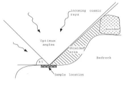
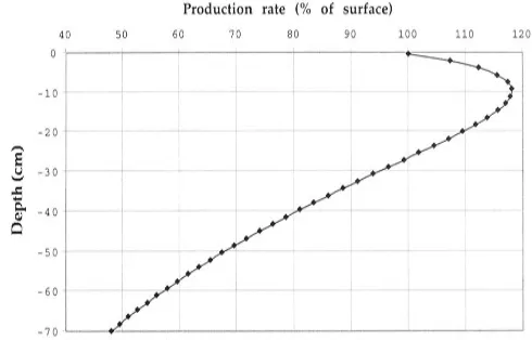
3. 9 Incident angles of the incoming cosmic rays on a rock surface 3.10 Build-up of Chlorine-36 through a rock. . . . . 3 .11 Location map for l\!Ici\!I urdo Sound and the Scott Coast 3.12 Chlorine-36 ages from Cape Bernacchi
3.13 Chlorine-36 ages from :VIarble Point
Vl
31
32
37
39
41
46
47
48
50
51
53
56
LIST OF FIGURES
3.14 Chlorine-36 ages from Dunlop Island 3.15 Chlorine-36 ages from Cape Roberts 3.16 Chlorine-36 ages from Cape Ross ..
3.17 Radiocarbon and Chlorine-36 samples at Cape Ross 3.18 Adjusted chlorine-36 ages for McMurdo Sound
3.19 Chlorine-36 ages with 5,000 years removed .. .
3.20 Relative sea level curve from Vestfold Hills .. . 3.21 Chlorine-36 ages from all McMurdo Sound sites. 3.22 Three possible exposure histories . . . .
3.23 Possible exposure histories for samples from Marble Point 3.24 Exposure histories predicted from the third forward model .
.. Vll 57 58 59 60 61 62 63 65 68 70 71
4.1 Flow chart of modelling process . . . 78
4.2 Schematic diagram of grounded ice below sea level 80
4.3 Gravitational attraction of sea level to an ice sheet 81
4.4 Sketch of the different contributions to the sea level change 82 4.5 Rebound direction of the Earth after the melting of an ice sheet 84
4.6 Characteristic sea level curves . . . 85
4. 7 Sketch of loading of a continental shelf . 88
4.8 Schematic diagram showing the effects of an ice sheet on a continent 89
4.9 Predicted relative sea levels from the Huybrechts (1990) ice model 93
4.10 Relative sea level from two different reconstructions of the Northern Hemisphere ice sheets . . . .
4.11 Maximum reconstruction from Stuiver et al (1981) 4.12 Ice surface reconstruction of Huybrechts (1990) ..
4.13 Nakada et al. 1999 reconstruction showing the ice thickness 4.14 Predicted relative sea levels from distal Antarctic ice . . . 4.15 Predicted r.s.l. from all ice outside the Ross Embayment .
4.16 Predicted relative sea level curves from ice outside of the Ross Embay-ment only . . . .
4.17 Three possible melting histories
96 97 98 99 100 101 102 103
5.1 Contour plots of predicted relative sea level 106
5.2 Field observations providing ice sheet constraints 108
5. 3 Ross Embayment drainage basin . . . 111 5.4 Relative sea level predictions comparing grounding line movement 112 5.5 Predicted r.s.l. curve from the Maximum reconstruction of Stuiver et.
Vlll LIST OF FIGURES
5.8 Predicted relative sea levels from variations on the Stuiver et . al. (1981)
reconstruction. . . 116 5.9 Early melting predictions . . . 117 5.10 Predictions of the r.s.l. in McMurdo Sound from late melting. . . 117 5.11 Predictions of relative sea levels from a modified melting history 118 5.12 Predicted relative sea level curve ofHuybrechts (1990b) in the far-field. 119 5.13 Illustration of a block of ice sitting on a surface . . . 120 5.14 Location of ice blocks on the Nakada et al (2000) reconstruction . . . . 121 5.15 Relative sea level curves for the reconstruction of Nakada et. al. (1999)
with blocks of ice added. . . 122 5.16 Predictions of-the relative sea levels with extra ice to the south 123 5 .1 7 Predictions of the relative sea levels with extra ice to the north 124 5.18 Predictions of the relative sea levels with extra ice to the east 125 5.19 McMurdo Sound with proposed ice flow direction . . . 126 5.20 Ice thickness~s at the LGM for the simple block model. 129 5.21 Predictions of the r.s.l. in McMurdo Sound for the simple block model. 130 5.22 Predictions of the r.s.1. in Terra Nova Bay for the simple block model. 130 5.23 Predictions of the r.s.l. at Cape Ross for the simple block model. 131 5.24 Contour plots of the Ross5 ice sheet reconstruction . . . 133 5. 25 Contour plots of the Ross5 ice sheet reconstruction . . . 134 5.26 Predicted relative sea levels for the Ross5 reconstruction 135
6.1 Present day r.s.l. change in the Ross Embayment from the Ross5 model 142
List of Tables
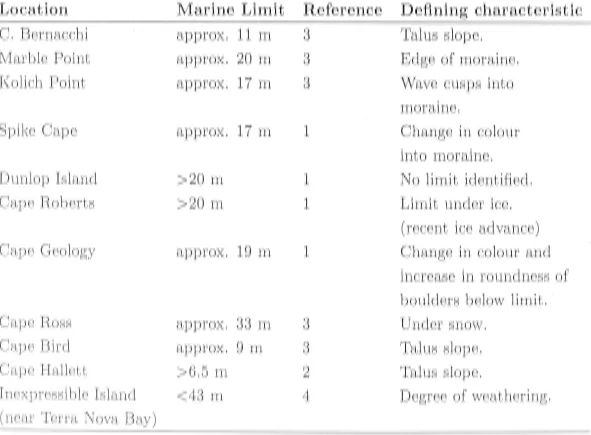
2.1 Table of marine limits . . . 10
3.1 Radiocarbon ages obtained from samples in the Ross Sea 35
3.2 OSL results . . . 45
3.3 Chlorine-36 production rates 52
3.4 Ages for surface exposure dating 55
3.5 N values for MP . . . 67
3.6 Exposure and burial histories for three scenarios 67
3. 7 Times of exposure and burial for two samples from Marble Point. 69 3.8
4.1
4.2
Erosion amounts for model 3 . . . .
Earth models used to determine Earth model dependency Predicted relative sea levels from the Earth models
73
91
92
B.l Measured chlorine ratios 156
B.2
%
K20 values measured 157B.3 Table of Major element analyses for the surface exposure samples . 159 B .4 Analyses of selected rocks for trace elements . . . . 160
B.5 Major element values (%) for the carbonate samples with the undissolved
sediment (non-carbon0te) removed . . . 161
B.6 Measurement values and production rates for all the samples 169
C.1 Sample locations and heights . . . 172
Chapter
1
Introduction
How big was the Antarctic Ice Sheet at the Last Glacial Maximum? Where was the ice located? How much ice was there? These are questions of immediate relevance to our understanding of recent climate changes on Earth and current debates on how climate may change in the future. To understand the ice sheets, how they effect and are effected by the climate, and what influence the ice sheets have on sea-level is important for modelling the climate system. Yet the answers, the fundamental data which must underpin the debate, are not easily obtained. This thesis addresses some of these issues concentrating on the change in ice volume from the Ross Embayment sector of the Antarctic Ice Sheet since the time of the Last Glacial Maximum. This sector is an important part of the Antarctic Ice Sheet extensively draining both the West Antarctic Ice Sheet and the East Antarctic Ice Sheet. It may also have had the largest retreat area of the Antarctic Ice Sheet since the Last Glacial Maximum and possibly the largest ice volume change as well, of any part of Antarctica.
1.1
Why the Antarctic Ice Sheet
Antarctica, and the Antarctic Ice Sheet , plays an important role in influencing the global climate. The ice sheet stores a vast quantity of water that can be released through global warming. With much coastal development occurring within a few metres of sea level a loss of only a small fraction of this ice volume has the potential to greatly alter coastal areas globally and to impact on large populations. By knowing how the Antarctic Ice Sheet behaved over the last glacial cycle we provide the basis for making informed predictions of how it may behave in the future.
A key element in Antarctica's direct effect on the world climate is the global ocean circulation. Sea-ice formation around the edge of the continent leads to the production of cold, relatively saline water that sinks off the edge of the continent and circulates northwards to modulate the flow of the warmer surface currents that in turn influence the global climate. Thus, any changes in the rate of deep-water formation around the
2 CHAPTER 1. INTRODUCTION
Antarctic margin impacts directly on global climate.
Sea levels have been measured to be around 120 to 130 m lower at the Last Glacial Maximum (Fairbanks 1989; Chappell and Polach 1991; Yokoyama 1999; Nakada and Lambeck 1987). A large part of this sea level change is due to water released from the Northern Hemisphere ice sheets which are relatively well defined compared to the Antarctic Ice Sheet. The last Northern Hemisphere Ice Sheets consisted of the Lauren-tian, InuiLauren-tian, and Cordillerian ice sheets over North America; Fenoscandinavian and Barents-Kara ice sheets over northern Europe; the Greenland Ice Sheet, and smaller ice caps on the British Isles , Greenland and Iceland. Evidence obtained from palaeoglaciol-ogy of large-scale flow-generated lineations (Boulton et al. 2001), relative-sea-level curves from beneath the former ice sheet (Dyke and Peltier 2000), continental shelf deposits (Sejrup et al. 2000) , marine limits from beneath the former ice sheet (Cofaigh 1999), stratigraphy and dating (Forman et al. 1999) etc. has made it clear that the history of these ice sheets is complex. However much more is known about the history of ice locations and volumes for the long vanished Northern Hemisphere ice sheets than for Antarctica.
Most estimates for the Northern Hemisphere ice sheet component of sea level rise since the Last Glacial Maximum are around 80 to 90 m equivalent sea level (Nakada and Lambeck 1988; Tushingham and Peltier 1991), leaving 30 to 40 m equivalent sea level to be sourced elsewhere on Earth. Limits have been placed on ice in the other possible locations such as Tibet (Kaufmann and Lambeck 1997). These sources are minor on a global scale with a maximum model for an ice sheet over the Tibetan plateau containing 6 m equivalent sea level. This leaves a substantial amount to be attributed to the Antarctic Ice Sheet (25 to 30 m). Because of this discrepancy and field evidence in Antarctica itself, there is general agreement that the Antarctic Ice Sheet was greater at the Last Glacial Maximum than at the present day (Stuiver et al. 1981, Bentley 1999 , Berkman et al. 1998, and Anderson et al. 2002). The present-day ice volume in t he Antarctic Ice Sheet is equivalent to about 70 m of global sea level rise so the Last Glacial Maximum volumes may have been as much as 45% larger than the present ice sheet.
Where, then, was t he extra ice located in Antarctica? The ice sheet itself can give us some information through ice cores which, depending on where they are located, can provide a record back more than 400,000 years (Petit et al. 1999). Ice core records from the interior of the ice sheet indicate that little change in elevation has occurred at the ice domes, and possibly a reduction in altitude by about 100 m in central East Antarctica ( J ouzel et al. 1989) . During the Last Glacial Maximum sea ice extended
1.1. WHY THE ANTARCTIC ICE SHEET 3
the coast is provided by exposure ages of bedrock and erratics (e.g. Brook et al. 1995). Evidence for the ice extending further onto the shelf than today, and in some cases out to the edge of the shelf, is provided by high resolution surveys of the shelf floor ( e.g. Anderson et al. 2002).
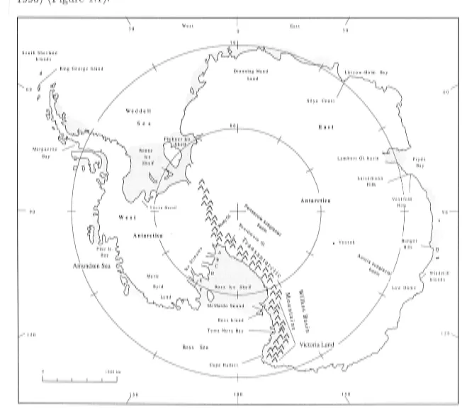
Records of Antarctic Ice Sheet retreats and advances can also be found on ice free areas. Many mountains and valley walls have records of former ice levels in the form of trimlines and lateral moraines (Bentley and Anderson 1998, Denton et al. 1989, Stone et al. 2003). Coastal areas provide moraines, ice scoured bedrock and erratics recording advances (Sawagaki and Hirakawa 1999). In areas around the edge of the continent where crustal rebound has exposed formerly glaciated surfaces that were below sea level immediately after melting, relative sea level changes can be documented from lake cores. The cores contain sediments that record the transition from marine to freshwater conditions. These lakes are found in the Vestfold Hills and Larsemann Hills (Zwartz 1995) (Figure 1.1).
Sou th She l land
Is land s
/ King Geo r ge Is land
60 a a(J
fl
Bay
90
Ba y
Amundsen Sea
1 20
30
Weddell
West
1
Antarctica
Ma ric Byrd
I 000 km
)50
West
Ross
Dronning Maud
Land
80
I 0
Ea st
30
SOya Coas 1
East
Lambert GI. basin
Hills
Antarctica
150
\
Figure 1.1 : Location map of the Antarctic continent
60
Vest f o ld
[image:17.1192.84.736.458.1034.2]4
160 °
Inexpressible Island
·-
a..0
....
0
>
Dry Valleys
CHAPTER 1. INTRODUCTION
165 °
170 °
100
I
Cape Adare
ROSS
SEA Q
Franklin Is
Beaufort Island McMurdo 0
Soood ~ l a o d
11 Ross
~ 6'..._ White Island Black Island
Ice
Shelf
70 °
Figure 1.2: Location map of the Ross Sea.
Offshore, core samples and seismic work can differentiate between formerly ice
cov-ered land, ice shelf or open water conditions to tell where the ice sheet was located
at different times (Licht et al. 1996 ; Anderson et al. 1992). Through studying these
sediment packages an indication of the location of the ice margin and the timing (where
true or relative dating is possible) of the fluctuations of the ice margin through time
can be obtained . I(nowing the ice margin is valuable in estimating the volume of ice in the ice sheet.
This thesis focuses on the Ross Embayment area, specifically field lo cations south of
Terra Nova Bay (Figure 1.1). The drainage basin comprises a grounded ice sheet over
East Antarctica, part of which drains through the north-south trending Transantarctic
por-1.2. OUTLINE OF THESIS 5
tion of the ice sheet over West Antarctica also drains into the ice shelf and contributes to the ice loading in the Ross Embayment. The Ross Ice Shelf calves over a wide front in the Ross Embayment ( see Figure 1.1). Part of the Ross Ice Shelf ( the McM urdo Ice Shelf) presently calves at the southern end of McM urdo Sound, close to the field locations.
The main field sites in this thesis are along the coast of McMurdo Sound with an additional location further north at Cape Hallett. In the Ross Embayment there are trimlines of former ice levels in the mountains which provide ice sheet height constraints (Denton et al. 1989), sediments on the continental shelf which provide grounding line constraints (Licht et al. 1996, Anderson et al. 1992), ice-shelf debris which provide timing constraints (Kellogg et al. 1990), drift sheets providing constraints on ice sheet extents and timing (Stuiver et al. 1981; Brook et al. 1995) and raised shorelines which indirectly constrain crustal rebound amount and timing. Together, these different pieces of evidence provide direct and indirect constraints on the history of ice volumes and a starting point to establish ice locations within the Ross Embayment.
1.2
Outline of thesis
The observational evidence for the limits and thickness of the past ice sheet over the Ross Sea Embayment is fragmentary in time and space, and some of the observational material provides only indirect measures of the ice extent. In the absence of a compre-hensive data set we therefore use mathematical models to relate the observed quantities to parameters that define the ice sheet and which can be used to interpolate between the fragmentary evidence. In this thesis it is mainly the shoreline height-age relation-ships that are used to constrain the ice sheet. The position of past sea-level relative to its present position is a function of changes in ocean volume and of land movements. Both, in the absence of tectonic processes, relate to the ice history through the eustatic change and through the isostatic rebound of the Earth to the changing ice-water load. In this case the model links the relative sea level change to ice history through the equations governing the response of the planet to loading and the equations governing the redistribution of the ice and water load as ice sheets grow or decay. In a complete model the ice sheet evolution is expressed by the equations of ice flow and ice accumu-lation drawn by a particular climate scenario. Ideally the ice-earth models should be coupled: the ice thickness that can accumulate in a function of the amount of deforma-tion beneath the growing ice load, but to date fully coupled models have not yet been developed and the two aspects of the modelling are usually carried out in an iterative manner.
6 CHAPTER 1. INTRODUCTION
spatial and temporal distribution of field evidence, as for the British Isles (Johnston and Lambeck 1999). In many other situations unique solutions are not possible. For example, a particular sea level curve showing a falling sea level for the past 6,000 years could mean that a considerable amount of ice was removed over a large area at some remote place or that a small near by ice load was removed in more recent time.
This is the case for the Ross Sea Embayment and instead of using inverse methods we use forward modelling methods to test glaciological models based on different field-data sets and on different ass umptions about the mechanics of ice sheet formation. From discrepancies or agreements between the observed and predicted sea level change inferences are then drawn about the past ice cover over the area.
The success of this approach depends on the availability of good quality sea level curves from lo cations for which different isostatic responses are anticipated: for example from sites well within the former ice margin and from near the ice margin. Secondly, it requires observat ional data that extends as far back in time as possible in order to constrain the early part of the deglaciation history. But in the case of Antarctica the observational evidence is very limited and is difficult to access. At the time of starting the thesis work t he principal evidence was that for Terra Tova Bay (Baroni and Orombelli 1991 ) where the record extends back to 7,5 00 14C years BP. Later the results of 14C dating of shells and seal fur by Hall and Denton (1999) became
available. In between I had started a fieldwork program collect ing relat ive sea level observations in an area to the south of Terra Nova Bay and I used three different dating methods - 14C of mollusc shells and p enguin eggshell, optically stimulated luminescence
( OSL) of beach sands, and cosmogenic exposure age dating of ro ck platforms and beach boulders. Both the OSL and cosmogenic exposure age dating methods were essentially exploratory methods at the time . The rationale for this was that each of the methods have limitations when applied to Antarctic materials and that the cosmogenic exposure age dating has the potential of extending the observational record further back in time.
1.2.1 Thesis layout
In this thesis the field work and dating that contributes to the observed relative sea le\·el cun·e is presented first. This allows my field observations, and other workers obsen·ations, to be described and used as constraints in making the ice sheets that are used as input to the glacio-hydro-isostatic modelling process presented in the second half of the thesis . The obsen ed relative sea level curve is also critical for evaluating the validi y of the ice-sheet models.
The role of isostasy in ice sheet evolution and sea level change is discussed from both a spatial and a temporal perspective in Chapter 4. Understanding these concepts is necessary for the detailed description of the glacio-hydro-isostatic modelling program.
1.2. OUTLINE OF THESIS
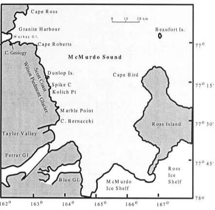
0 10 20km
M cM urdo Sound
Beaufort Is.
0
Ross Ice Sh elf
- 77°
- 77° 15'
77° 30'
[image:21.1192.181.623.123.555.2]• 77° 45'
... _...,.._ __ ... ---_____ .,;;;a_.._ _ _ ... _______ • _ _ _ ___,78°
162° 163° 165 o 166° 167°
Figure 1.3: Location map for McMurdo Sound and the Scott Coast.
such as the ice and water loading of continental shelves.
7
As mentioned earlier in this introduction, the ice sheets of the Northern Hemisphere impact on Antarctica in terms of sea level changes, so the possible effects of varying the models of the Northern Hemisphere ice sheets are examined. That part of the Antarctic Ice Sheet outside of the Ross Embayment area will also impact on the Ross Embayment, not only through changing the sea-level, but also by direct loading of the Earth's surface. Possible variations of the Antarctic Ice Sheet are examined to determine the scale of errors which result from using different models.
Chapter
2
Field Observations
2.1
Victoria Land Coast and Islands
The coastal area along the Victoria Land Coast is ice free in only a few places (Mabin 1986). These ice-free areas consist of low rocky coasts, beaches and high rocky cliffs ( Gregory et al. 1984).
Raised beaches were first recorded by David and Priestley (1914) in the McMurdo Sound area and these were first examined in detail by Nichols (1968) and Kirk (1990). A summary of the early work and radiocarbon dating can be found in Stuiver et al. (1981). Further north, in Terra Nova Bay, Baroni and Orombelli (1991) examined and extensively dated these raised beaches.
This chapter describes and interprets the characteristics of the coastal areas with emphasis on the features and regions examined for this thesis. A description of the sediment sources, morphology and preservation of the beaches is given with examples from the Scott Coast ( western side of McM urdo Sound). The boulder pavements, the rock platforms and the glacial moraine above the marine-influenced area are describ ed with relevant details for the dated sites. Further descriptions of each site visited ( Cape Bernacchi, South Stream, Marble Point, Kolich Point, Spike Cape, Dunlop Island, and Cape Roberts (all in McMurdo Sound); Cape Geology and Cape Ross in Granite Harbour (to the north of McMurdo Sound); Cape Bird on Ross Island and Cape Hallett in Northern Victoria Land) can be found in Appendix A.
2.2
Marine Limit
The marine limit is the highest altitude at which the sea has had some recorded influence on a coast. This elevation is a function of the amount of uplift of the coastline that has occurred since the coast became ice free (from both sea-ice and any land-based ice). The marine limit therefore, is dependent on both the amount of relative-sea-level change and on ice conditions at any particular location. The marine limit is very clearly defined
10 CHAPTER 2. FIELD OBSERVATIONS
in some places (e.g. Kolich Point - Figure 2.1.) where there is an abrupt change from rounded beach boulders of only a few of lithologies (below the marine limit) , to poorly sorted , angular clasts of many sizes and lithologies ( above the marine limit). At Kolich Point , even cusp features ( wave-scalloped areas) are preserved at the marine limit. The majority of marine limits, however, show more subtle changes, with a change in slope or the angularity of the material being the best indicators of the marine limit. The marine limit is often easier to pick from a distance or on aerial photographs (Figure 2.2) than up close. To the south between Cape Bernacchi aI).d Explorers Cove, and also on Cape Bird and Cape Hallett, the marine limit is unclear because of a talus slope or a steep hill of moraine that has subsequently covered the landward edge of the marine influenced area. At these sites the limit of marine influence is defined as the area up to the edge of the talus slopes. Table 2.1 shows the marine limit at each site and how t he marine limit is defined there.
Location
C. Bernacchi Marble Point
Kolich Point
Spike Cape
Dunlop Island
Cape Rob erts
Cape Geology
Cape Ross
Cape Bird
Cape Hallett
Inexpressible Island
(near Terra ova Bay)
Marine Limit
approx. 11 m approx . 20 m
approx . 17 m
approx. 17 m
>20 m
>20 m
approx. 19 m
approx. 33 m approx . 9m
>6.5 m
<43 m
Reference 3 3 3 1 1 1 1 3 3 2 4
Defining characteristic
Talus slope.
Edge of moraine.
Wave cusps into
moraine.
Change in colour
into moraine.
o limit identified.
Limit under ice.
( recent ice advance)
Change in colour and increase in roundness of boulders below limit. Under snow.
Talus slope,
Talus slope.
Degree of weathering.
Table 2.1: Marine limits on the Scott Coast , Cape Ross, Cape Bird , and Cape Hallett.
Refer-ences: 1. Nichols (1968); 2. Kirk (1990); 3. This thesis; 4. Claridge and Campbell (1966).
2.3
Beaches
[image:24.1192.93.684.464.899.2]2.3. BEACHES 11
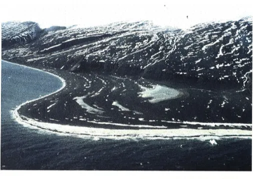
Figure 2.1: The marine limit at Kolich Point. The marine limit here is defined by the change from multiple lithologies, angular clasts and greater weathering above the marine limit to brown, rounded clasts with sand interspersed below the marine limit. The view is from above the marine limit looking down the slope such that the foreground shows the region above the marine limit and the background shows the region below. The size of the larger boulders in the photo are approximately 0.5 min· diameter.
active Antarctic beach is not dissimilar to that of a temperate beach (Figure 2.3) and is predominantly composed of a sand and gravel mix, with small boulders. Generally, the beaches are clast supported (boulders with interstitial sand) with clast sizes up to about 30 to 40 cm in the more active areas. In the front of the beach there is a
[image:25.1192.175.588.128.641.2]12 CHAPTER 2. FIELD OBSERVATIONS
Sea 1c'e
Figure 2.2: Aerial photo showing the raised beaches and marine limit at and to the South of Cape Bernacchi. On the right shows the sea ice, raised beaches up to the marine limit and the pitted moraine above the marine limit.
than it is lower down on the beach. The top of the beach is typically q_uite flat , with a gentle slope back towards t he swale behind the berm. This swale is made up of finer overwash material.
2.3. BEACHES 13
Figure 2.3: Sketch of a profile through a typical Antarctic beach. The scale is vertically
exaggerated but shows the area where sea level is normally on the beaches and the high berm formed during storms. The height of the storm berm varies between about 0.5 min low energy areas to about 4 m in exposed sites. The distance between the berms is dependent on the overall slope of the shore and the wave energy. Cusps form from wave action.
layered, although the characteristics of the layers are usually similar between different layers in a beach, such as the roundness of the pebbles.
Successions of beaches along the shores of McMurdo Sound occur commonly on short stretches of coastline between rocky headlands where the sediment supply is sufficient. The raised beaches consist of a series of 3 to 5 ridge and swale systems up to the marine limit (Figure 2.4). The source of the material that forms Antarctic beaches is likely to be a local reworking of moraine and littoral sediments (Kirk 1970). However, longshore currents supply sediments to a few beaches such as at Kolich Point and Cape Hallett, and sea-ice transports material from gravel size to boulders. The largest boulders on the beaches are erratic boulders up to several metres in size.
In the case of the Scott Coast on the western side of McM urdo Sound the local rock types found in the beaches are granite, granodiorite, dolerite, marble, schist, gneiss, quartzite and the occasional piece of volcanic rock - some of which is sea-ice rafted in from Ross Island. At Cape Bird and Cape Hallett the local rock type is volcanic ( olivine basalt to trachytes at Cape Bird and basanite to basalt to hawaiite at Cape Hallett (Le Masurier 1990)).
The dominant beach-forming process is water and wave action, although ice is a feature of Antarctic beaches and ice push features can sometimes be recognised. Ice push features are formed on the active beach, and occasionally are preserved on the raised beaches, such as at Cape Ross. These ice push features occur when a large piece of shore-attached ice is bulldozed up the beach from the breaking-up sea ice. The ice and gravel mix forms an ice-cored 1nound at the end of the bulldozed area with a flat area seawards of where the ice was. Large pieces of stranded ice can also be incorporated into the beaches which, when they melt , form melt-out pits in the beaches.
14 CHAPTER 2. FIELD OBSERVATIONS
Figure 2.4: Photo looking at the southern point at Cape Bird, Ross Island. A series of raised beaches extend out and around the cape to a height of about 9 metres above present day sea level. The small patches of snow or ponds pick out the swales behind each ridge. The marine limit is at the base of the small cliffs. For scale the distance from the cliffs to the point is approximately 500 m.
Geology. Figure 2.5) are examples of a lack of development due to fewer open water seasons. At present the beaches in McMurdo Sound become ice free in mid-January and the sea ice re-freezes between late-February and early-March. When (if at all) an area of sea ice breaks out depends somewhat on whether it is a whole bay or only a section of an exposed straight coastline that needs to break out. The true break-out times of the sea ice at the head of McM urdo Sound are difficult to estimate in the
-modern era due to ice-breaking activities by ships that loosen ice earlier in the season than would otherwise occur. Extrapolating break-out times into the past, therefore, becomes even more difficult .
[image:28.1192.127.633.134.492.2]2.3. BEACHES 15
Figure 2.5: Photo of poorly formed ridges at Cape Geology. The marine limit is marked by
the yellow line on the right-hand-side of the photo. The marine limit is also visible from t he roundness of boulders below the marine limit.
major ridges. These have probably formed in events smaller than those that caused the larger ridges , but not large enough to form a true ridge.
The beaches along the Scott Coast range from very low energy environments ( very sandy with little other material) to very high energy environments (large boulder banks). In general, the main fetch (wave generation area) direction is from t he nort h east in McM urdo Sound and this is reflected in the higher energy levels of t he north-east facing beaches. The wave energy is also reflected in the morphology of the beach ridge (Figure 2.6 ). Lower energy beaches are flatter and wider. In the case of Spike Cape t he height of the beach ridges reduces significantly where the former-islands (now penin-sulas) stopped waves originating from the dominant fetch direction. On t he sout hern side of all the capes there is only the short fetch of McM urdo Sound ( in most cases less than 80 km ) and often the sea ice does not break out of the sout hern side of t he point so the beaches there tend t o be sandier. The same sandy t endency is seen in bays where the sea ice rarely breaks out (such as in Explorers Cove). Low energy beaches and shore deposits still form in these locations from t he little wave energy propagated through the sea ice into the small ice-free st retch at the wat ers edge t hat develops in the summer.
16 CHAPTER 2. FIELD OBSERVATIONS
Figure 2.6: Top: High rocky berms found at Kolich Point. These berms are up to 5 m in
2.3. BEACHES 17
The height of the berm above the relict beaches can vary from half a metre to several metres, depending on the wave energy that formed the beach. Because of this height variation, the berm tops are not reliable measures of beach height and a feature such as the break in slope in front of the berm that occurs on both the modern and relict beaches is a more reliable indicator of the relative sea level on the relict beach.
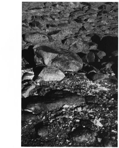
The extent of weathering on the raised beaches must also be accounted for. The wearing down of boulders and filling of the swales can give a false impression of the beach berm height and provides another reason not to use the berm for a measure of beach height. The amount of weathering of the beach boulders is also an important consideration for surface exposure dating because an incorrect estimate of the erosion depth will lead to an incorrect age ( see chapter3). Weathering of the beaches increases with height above sea level and the boulders on the top beaches are heavily weathered in places with 'tails' of crystals downwind of the predominant southerly wind direction in the area ('tail' size depends somewhat on boulder material - marble weathers fastest). In many cases the boulders have weathered into a well rounded form. Coarser grained rocks, such as granite, weather by individual crystals breaking off but the marbles also weather by a process of losing flakes. Endolithic algae grow at a depth of 1 to 2 cm within the marble rocks, providing a weak layer at which the rock will flake. Phonolithic ( wind sculpting) weathering, common in many places in Antarctica, does not occur below the marine limit because this type of weathering requires a long time of exposure. Chemical weathering is active on the beaches as well, but the physical weathering is dominant. Iron staining is an obvious feature here and appears to be most extensive on the southern facing beaches. All the beaches have a deflation surface of small pebbles less than 30 mm and individual crystals weathered from the surrounding cobbles and boulders (Figure 2. 7). The deflation surface is formed by the wind scouring of the finer material, similar in appearance to pebbled concrete.
2.3.1
Sandy beaches
18 CHAPTER 2. FIELD OBSERVATIONS
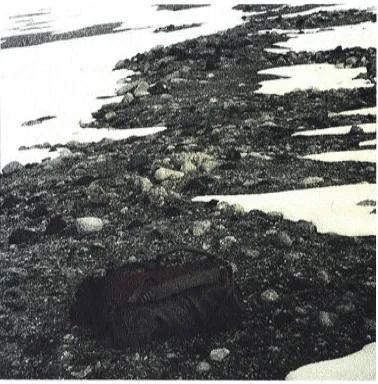
Figure 2. 7: Deflation surface on the beaches at Marble Point with a gravel surface and small
scattered boulders. The view is along one of the raised beaches on the south side of Marble Point. Snow to the left-hand-side fills the swale from the seaward beach and the leading edge of the beach berm. The length of beach shown in the photo (to the edge of the hill) is approximately 800 m and a day-pack is in the foreground for scale.
more boulder-rich deposits down a succession of relict beaches (progressively younger). This indicates that it is likely that the sea ice did not break out progressively more over time but rather t hat seasonally open-water conditions have existed for the entire time of beach formation.
2.4. BOULDER PAVEMENT
19
2. 3. 2
Boulder beaches
Boulder beaches are at an extreme end of the beach types seen along the Scott Coast. They retain all the features of a sand and gravel beach but have a larger typical clast size which can be up to a metre in diameter. On one site where the boulders have been used for surface exposure dating ( Cape Bernacchi) the beach faces north-east and is seasonally open to the Ross Sea. Cape Bernacchi appears to become ice-free regularly ( on its north-east side) so will be exposed to large storm events capable of building the large rocky berms. There are three wide relict beach ridges above the present-day beach. Any potential higher beaches than this are unformed or covered by the edge of a very steep moraine-covered hill on the back of the beaches with a minor talus slope. Cape Ross is the other sampled location with boulders of a sufficient size for surface exposure dating. This is on the northern side of Granite Harbour and is ice free much earlier in the season than the rest of McMurdo Sound.
2.4 Boulder pavement
Raised shorelines feature boulder pavements in varying stages of development. As their name suggests, they are very flat surfaces formed by the planing action of sea ice which removes the tops off the boulders. In the case of Cape Roberts, where the boulder pavements are superbly developed (Figure 2.8), the boulder pavements consist of former beach ridges made of interlocking boulders . The underside and sides of these boulders are rounded in the usual way of beach boulders but the tops are smoothed flat. There are no ice scours on the top of the boulders but a polished surface is also not developed. There is very little sand on these ridges, only gravel between the boulders and in the swales. The boulder pavements are developed on both the northern and southern sides of the cape whereas the present day beach is well formed only on the northern side. At Cape Roberts the present beach on the northern side is also a boulder ridge but rather than showing evidence of erosion it is a depositional feature, suggesting a change in sea ice and erosion conditions. Each boulder pavement at Cape Roberts was sampled for surface exposure dating.
2.5
Rock Platforms
20 CHAPTER 2. FIELD OBSERVATIONS
...
-<ll>~'t¥;:
, 1'!':"t''~··"""'
~ -... ,,.,
~- ·....,_; '
... ~~> , '1.'7~ ~~',;-tt~••'"'"'r ;.,,#.,,.~ • 4'\'
"' "
Figure 2.8: Boulder pavement at Cape Roberts. View along one of the raised beaches on the
northern side. Note the very flat tops on the boulders with rounded sides. Beaches extend for several hundred metres. The rocky berm on the right-hand-side in the middle ground is the active beach.
If the bottom is rock the ice cuts and polishes the rock into a step. At a later stage some wave action may modify the ice cutting, but the polish retained suggests this is minimal. Because the scouring occurs at the base of the sea ice approximately 2 m below sea level, the platform that correlates to a beach ridge is actually below the beach ridge in true height by about 2 to 3 m, depending on the wave energy that formed the beach. The sampling of wave/ice cut rock platforms for dating purposes has not been attempted in the Antarctic before, although has been successfully used elsewhere -such as on the main rock platform in Scotland (Stone et al. 1996).
2.5.1
Deltas
2.5. ROCK PLATFORMS
sea ice
0
water
\
scou ring area
\
shore attached ice
height of corresponding beach
21
Figure 2.9: Formation of rock platforms by ice scouring. Wave action moves the loose sea ice in an elliptical motion over the scouring area, eroding the bedrock.
from ice melting, of the surfaces in the swales . The beaches are wide ( approximately 40 m) , composed of well-rounded clasts, with a rise of approximately 2.5 m. The beaches become less distinct towards the delta as they decrease in height and grain size until the ground becomes hummocky with ice-melt pits up to 30 cm deep. On the south side of the stream the beaches are slightly more confused due to multiple streams from the hill slope behind. The ground is well sorted, but pitted, and appears to merge into the highest beach ridge .
The flattening of the beaches and the reduction in grain size suggests a lowering of energy towards the delta. A low wave energy environment with little movement of material would be required to ensure the preservation of the deltas as the sea-level dropped. This could be achieved by a reduction of wave energy levels as waves refract around the Marble Point headland (the dominant wave-front direction is from the north-east). In such a scenario waves arriving in the area of the delta would have very litt le energy for reworking the deposit .
Aerial photos of the beaches on the northern and southern sides of the delta show that they are at approximately the same altitude. Slightly further up t he valley, skirting the top end of the delta, the marine limit probably lies close to but above the delta because it contains marine shells . This would put the marine limit around 15 m asl which is between the limit seen at Marble Point (around 20 m asl) and the 12 m seen at Cape Bernacchi. The surface of the delta is almost as high as the surrounding beach ridges, indicating that it must be younger than the top-most ridges. Steps lower in the delta ( closer to present day sea level) that could be interpreted from the aerial photo as a marine limit may actually be lower beaches.
22 CHA P TER 2. FIELD OB SERVATIONS
delta
ma rine li mit Sea Ice
mo raine beach ridges
N
l
Figure 2.10: Aerial photo of the delta at South Stream, Scott Coast and the surrounding beach ridges. The delta edges are clearer on the ground (see the next figure) but this view shows the marine limit and the beach ridge height lessening towards the head of the bay. The ridge-like appearance across the delta are stream cuts in-filled by snow in this image. Width of the photo is approx. 4 km.
size analysis shows an overall upwards coarsening trend but with a shift to a fining
se-quence in the middle part of the section. A coarsening trend suggests shallower water
or a higher water inflow (it can carry larger grains). A shallowing of water depth would
correlate well with relatively rapid delta formation. Fluctuations in the grain size can be interpreted as a function of changing environmental conditions supplying sediment. Diatom analysis shows a large percentage ( average 60%) of fresh water species with the remainder being of brackish or marine origin. There is a larger percentage of marine species at the base of the section. Deposition of the delta would occur in summer when the melt-water streams are flowing and this is when the diatoms would be growing as well. The large influx of fresh water into the near-shore area could provide conditions for the fresh-water and brackish-water diatoms to be deposited in a marine environment . This interpretation fits wifh the fresh-water algae found in the delta. Stuiver et al. (1981) have described this algae and have used it as part of their dating of the delta (later it will be shown that the ages are consistent with the shell dates).
2.6. ROSS SEA DRIFT 23
elliptica. The presence of these shells and the sediments and diatom assemblage indicate
that the delta formed in a marine environment.
2. 6
Ross Sea Drift
While glacial moraine information does not give direct evidence of the rebound along the coastal area, it can provide clues on ice sheet extents and the timing of the glacial advances and retreats. Positively identifying a moraine on a hillside with a particular glacial event ( in this case the last glaciation in the area) provides a limiting estimate of the maximum ice sheet elevation in the area. This in turn can be useful in constraining the total size of the ice sheet.
Denton et al. (1989) attempted to provide a constraint for the overall size of the Ross Ice Sheet by this method (see Figure 2.13) using information from the Reedy Glacier, Beardmore Glacier and Hatherton / Darwin glaciers that flow into the Ross Sea from the East Antarctic ice cap. By determining the youngest moraine in each valley and assuming a constant age for these, maximum limits of ice height in the Ross Sea have been obtained since the ice could not have been higher than the moraines at the outlet end of the glacier. Orombelli et al. ( 1991) examined the glacier profiles and moraines of the Terra Nova Bay region and provided constraints on the Ross Ice Sheet in this area.
The Ross Sea Drift is a term given by Stuiver et al. (1981) to the area covered by
the last expansion of ice in the Ross Embayment. Aerial photos of the region clearly show the Ross Sea Drift as a covering of sediments around the mouths of the valleys and coastal areas (Figures 7-4 and 7-5 from Stuiver et al. (1981) show this well). The drift sheet, characterised by numerous eskers and minor moraines, has end moraines around the McMurdo Sound region and in the Taylor Valley. The geographical distribution of the terminal moraines has been mapped, along with their heights above current sea level (see Figure 2.14). The Ross Sea Drift is described by Stuiver et al. (1981) in terms of its soil development characteristics ( very little development) and its boulder frequency and lithology. The dating of sediments from a pro-glacial lake dammed in the Taylor Valley (Stuiver et al. 1981) and from small ponds (Hall and Denton 2000b) have constrained the time of this drift sheet to the Latest Pleistocene.
2. 7 Hjorth Hill Moraines
24
Wilson Piedmont Glacier
Scale between top of delta and stream
5m delta
--
-
-
...-CHAPTER 2. FIELD OBSERVATIONS
moraine approx. marine limit
delta
Stream
delta
surface of delta
Figure 2.11: Top : Overlay for the photo of the South Stream delta. Bottom: Delta at South
Stream. The delta here is cut by modern streams leaving 'islands ' of the former delta. Snow
covers most of the bed of the stream in t he photo. Distance to the Wilson Piedmont Glacier is
2. 7. HJORTH HILL MORAINES
Stratigraphic Column
~
g Unit Descriptions
E Beddip
-;;; cO I.. mean grain siz
(phi)
\°"
6 5 4 3 2 I 0 -1 -2Sample location
i., "ij Foreset dip
(/) ..c
4.5 4.0 3.5 3.0 2.5 2.0 1.5 1.0 ... ··· ... ...
0 ... 10 I O I 0 0 0 I I O O 1 0 0 0 0 0 I I O O O O IO 1 0 0 o l - - - ---<
.. ... ...
.... ... ... ... ...
··· ... .. ... ... .. .. ... ... .. ...
'' '' ' '' ' ' ' ' ' ' '•' ' ' ' '•' '•' ''' A9
e O f I O I O O O I O I O O I t t O t O t I I I t I IO O 1 - - - <
··· ... , .. , ... ... .
• • • • • • • • • o • • • • • • 0 • • I O 0 • • • 0 • • • • 0 I O I O O I • • 0 0 • e I
Lag surface; subround-angular pebbles 2 - 40 mm dia. Oasts of quartz, marble, granite, dolerite.
MediUII\ sand, foreset bedded, poorly consolidated (unfrozen), subround-angular pebbles (dropstones) up to 40 mm throughout .
Fa resets, dip 56 deg. at 052 .
Laminated (3 - 6 mm) medium sand and silty sand, coarsening upwards.
Wedge of very coarse sand-fine pebbles, well rounded, cross stratified I cm beds alternating coarse/ fine, overall fining
h-rim+mmrrmWrrrmin
11
-;., 1
,t,~ _;... _~ _-_-_-_-_-_-_--~ upwards. Dip at top 28 deg. at W6, dip at base 38 deg. at 074.
A7
••••I••••••• I•••••• I• I••••• lU__ L _ _ _
·::.').<'\\:•::.'.':::: :·:~·,',' r===i] ~ e laminated mediUII\ sand.
:::::::::::•:•:•~;:,:•:•:•:-:::::1---
A6 ... ... ::::~:::::::·.·:~::·.· ··••,.••···•,.•··· ... ·· ... . , .. , ::::·.-:~···::~·::::::·.·:.'.' ····.. .. •, , ,• •··· .. •·· ... . . . ' ... ' ... · ... .;:::~-:-:-:-:.:.:-:·:-:-~:::
• t t • o IO I ' I • 0 0 o • I • ' • I • o o t • 0::::•:-:-:·::-)?\·:-:-:-:-:·:·:.:.::
...
• • • • • • • • • • • • • • ' 1 - - - -- l
... ' ...
. . . . . . ' ...
ice layer, 3-4 cm thick, fine sand / silt entrained within ice.
MediUII\ sand, alternating rippled and planar lamination 3 - 15 mm thick, cross stratified ripples. Ripple dimensions; wavelength = 7 -20 cm, amplitude = 6 - 25 mm. Basal 20 cm not rippled or laminated. Overall coarsens upwards.
lnterbedded, rippled, mediUII\ sand / silty sand, I - 2 cm beds, wavelength = 20 cm, amplitude = 2 cm.
Planar, 2 - 3 mm, laminated medium sand.
_)6. ... ...._ _ _ _ _ _ __ _ __ _ _
...
.. 0 ... ...
1---l
..
:::::::::~::::::;'::::
: : .·.o-. ·. ·,·::: :. ·. ·. ·. ·,·:: .· .·. ·. ·. ·.
... ... ... ... ... ... ... ... .... ... ... .... .. ... . . . ' .. .. ... .
• 0 • • I • o • t t I O • • o
... . . . . . . . . ' ... .
• •'''C3•· ·,., •• a.··, .... Q,
. . . , 1 - - - , ~
High angle (37 deg. apparent dip), cross stratified coarse sand.
Large block of ice entrained within unbedded mediUII\ sand.
Coarse sand fining upwards to mediUII\/ fine sand, small <!cm pebbles thoughout, occasional ripples.
Coarse sand containing small , <I cm subangular-subround pebbles, fining upwards to fine sand. Sharp basal and upper contacts .
Basal dip = 9 deg at 058 .
lnterbedded, ripple laminated fine / silty sand. Wavelength= 8
cm, amplitude = I cm. Thicker (3cm) upper layers. Contains complete
Adamussium colbecki shells.
Coarse sand layer, 1.5 cm thick, orange (oxjdi.sed) colour. Dip = 9 deg. at 058.
lnterbedded, ripple laminated fine/silty sand. Sharp upper contact.
lnterbedded fine sand and sil t, 3 mm laminations. Graded
0.5 contacts.
(fc - o
- 0
-Al
Dark, non-laminated silt. Contains small bivalves, blocks of ice and dropstones. Graded upper contact, basal contact not
exposed.
25
Figure 2.12: Stratigraphic column of section through the South Stream delta. From \iVebb
26
3500
3000
2500
?
~ 2000
~
"' ~ 1500
~
1000
500
0
- - - Reedy I ice surface
- - - - • Reedy II ice surface
- - - - • Reedy 111 ice surface
f\!\f\f\f\M\ Present ice surface
l\ce stream ~ \ce Sheet) .5 "'
',Nest }\ntarctlC §
0
::E
50 75
CHAPTER 2. FIELD OBSERVATIONS
----"' u "' c.. .9 "' u---
-
-
-
-EED'l GLACIER t'c Mountains)
R h Transantarc i
lOut\et Glacier thfoug
100 125
Distance from Ross Ice Shelf (km)
150 175
Figure 2 .13: Interpreted palaeo-ice surfaces of the Reedy Glacier ( flows into the Ross Sea about 86°S) from former glaciations. The former surfaces are only dated by relative dating and are referred to as the Reedy I, Reedy II, and Reedy III ice surfaces. Projections of the
ice surface to the Transantarctic Mountain front places a limit on how much ice was in the Ross Sea (it cannot have been higher than the lateral moraine) and likewise at the inland end (approximately where the nunataks are marked). Quartz Hills, Caloplaca Hills, and Polygon Spur are mountain ranges in the Transantarctic Mountains that are cut by the glacier ice. From Denton (1989).
produced a hummocky ground of meltout pits and stream beds. Sediments older than t he Ross Sea Drift appear higher on the slopes of Hjorth Hill and Hogback Hill. The lithology of these glacial sediments is the same as the lower sediments but the degree · of weathering and soil development is much greater. Brook et al. (1995) have taken 12 surface exposure dating samples from two sites in this area to compare the ages of older and younger moraines. The dates of the older moraine at Hjorth Hill range from 104, 000 to 567,000 and the younger moraine range from 8,000 to 106,000.
The moraines on these same hills show there is more than one set of moraines within
t he younger drift sheet and that there is some overprinting of glacial moraines onto ot her m aterial. Hall and Denton ( 2000a) have closely mapped and dated fresh-water algae from the various moraines. This mapping, together with my field observations , suggests t hat an ice sheet overrode the coast from the east and merged with the Wilson Piedmont Glacier , with various advances and retreats over the Late-Pleistocene and Holo cen e.
2.8
Wilson Piedmont Glacier
2.8. WILSON PIEDMONT GLACIER
Mt. Morning
McMurdo Sound
6 Kilometres .50
•
Ross Sea driftii
Older drift27
Figure 2.14: Location of Ross Sea drift and older drift sheets. After Brook et al. (1995).
The light grey is the Ross Sea drift from the last glacial period which extends up to 300m on Hjorth Hill and Hogback Hill, and into the Taylor Valley where the ice blocked the valley mouth between 23,800 and 8,340 14C years before the present (Hall, 1999b).
beach ridges. At four field sites visited the beach ridges extend beneath the glacier. In the case of Kolich Point the profile of a sandy beach ( shown in appendix A) comes from a point about 20 to 30 m from where this beach extends beneath the glacier. Old aerial photos of this area ( from the 1960 's) show that the whole area, extending almost
28
CHAPTER 2. FIELD OBSERVATIONS'rolling' motion over the surface and does not move any rock material. Similar evidence for this can be found to the north at Spike Cape and at Cape Roberts. Beaches at Cape Roberts show some sign of minor disturbance for 10 to 15 m away from the face of the Wilson Piedmont Glacier, but this is limited to the occasional rolling of the small boulders/ cobbles on the top of the beach ridge - the structure of the ridge remains unchanged. At this site there is evidence of water movement ( silt covering the rocks in places) which may have moved the surface rocks. At the southern part of the Wilson Piedmont Glacier there is less evidence of erosive power ( either way) of the glacier.
2.9
Summary
Observations from McMurdo Sound provides information about ice extents and former sea levels in a variety of ways. Evidence from glacial moraines in the surrounding valleys and along the hills of the Scott Coast area indicate that the Ross Sea drift, the ice sheet of the last glaciation, extended some 300 m above present-day sea level on this portion of the coast. Former sea levels are preserved up to an altitude of about 33 m at Cape Ross and decrease southwards to about 11 m at Cape Bernacchi and westwards to about 9 m at Cape Bird on Ross Island. Cape Hallett has a very low recorded marine limit. Below the marine limit raised beaches (typically 3 to 5 beaches) or correlatable rock platforms are found except where the ice-free land ends in cliffs. The formation time, sediment supply, formation energy and preservation are all important features of t he beach that must be known before a meaningful interpretation can be made about the local relative-sea-level change. It must have taken a change in conditions to preserve