A demonstration of the utility of fractional experimental design for finding optimal genetic algorithm parameter settings

A demonstration of the utility of fractional

experimental design for finding optimal genetic

algorithm parameter settings

DJ Stewardson1and RI Whitfield2* 1

University of Newcastle, UK; and2University of Strathclyde, Glasgow, Scotland

This paper demonstrates that the use of sparse experimental design in the development of the structure for genetic algorithms, and hence other computer programs, is a particularly effective and efficient strategy. Despite widespread knowledge of the existence of these systematic experimental plans, they have seen limited application in the investigation of advanced computer programs. This paper attempts to address this missed opportunity and encourage others to take advantage of the power of these plans. Using data generated from a full factorial experimental design, involving 27 experimental runs that was used to assess the optimum operating settings of the parameters of a special genetic algorithm (GA), we show that similar results could have been obtained using as few as nine runs. The GA was used to find minimum cost schedules for a complex component assembly operation with many sub-processes.

Journal of the Operational Research Society(2004)55,132–138. doi:10.1057/palgrave.jors.2601703

Keywords:genetic algorithms; scheduling; sequential experimentation; regression; optimization

Introduction

Design of experiments (DOE) techniques provide a systema-tic, effective and efficient approach to the investigation of a phenomenon.1 The approach is often sequential in nature, potentially increasing in complexity as the knowledge and understanding of the application and domain evolves.2The main advantages of the strategy are the savings in time and resources expended compared to other approaches and the resulting mathematical models that help users to better understand the phenomena under investigation more fully. This investigation demonstrates the application of a number of efficient experimental designs to re-address a previous application of DOE techniques within the optimization of the structure of a GA. The particular experimental designs considered within this investigation include: a two-level ‘full-factorial’ design with one centre point in nine experimental trials; a Box–Behnken design with 13 trials, and, a central composite with 15 trials. The focus is on demonstrating that these designs, in particular, the nine trial designs may be used with a fitness check of the model to assess whether there is any requirement to undertake further trials. In computer simulation work of this nature, there is no penalty from adding later trials, unlike the situation in industry where ‘blocking’ or ‘nuisance effects’ are often observed. By this, we refer to changes over time in the response that is being measured. In an industrial setting, for example, we may see different results at night, the next day, or because a shift has

changed. Material inputs may become different, environ-mental conditions may change, and thus adding the results of trials run at a later time may result in wrongful conclusions unless these potential effects are considered. In simulation work this is not an issue, running a program with the same parameters and the same initialization will always produce the same results. The paper suggests that a minimum number of treatments can be investigated which need only be added to later, if the initial analysis suggests that this is required, resulting in a considerable saving in time when investigating large and complex problems like this one. The paper goes on to show how, in this case, a reduced number of experimental runs would have produced a similar result to those found in the actual investigation. A brief description of the scheduling problem is given first, then we show how experimental design techniques were used to determine the ‘best’ structure of the GA and then the adoption of a sequential strategy is discussed. The use of this particular study as an example should, we hope, serve as a springboard for others to use these methods in other computer program optimization work. It has been over-looked by some writers that computer programs have good and bad ways of being written, and optimum programs can often achieve better results.

Scheduling problem description

Scheduling has been defined as ‘the allocation of resources over time to perform a collection of tasks’.3These types of problems are often difficult to solve because they involve complex combinatorial optimisation and can only be solved *Correspondence: RI Whitfield, CAD Centre, University of Strathclyde,

G1 1XJ.

E-mail: [email protected]

by non-deterministic polynomial algorithms. These pro-blems are well suited to solving by Heuristic means. In particular, the use of GAs has been shown to speed discovery of good solutions.

The work analysed here involved using the Genetic Algorithm (GA) to produce improved solutions for a large, computationally intensive scheduling problem,4,5 in which several other popular optimization techniques had been shown to produce very much inferior schedules. The GA used was based on a modification of the Goldberg algorithm6that includes a repair function to avoid infeasible solutions. The capital product being assembled had six levels of product structure, 46 components, 497 machining operations and 39 assembly operations, which were performed using 24 machine tools and one assembly area. The fitness function minimized the various cost penalties that were associated with either being early or late with the various components in the assembly.

Experimental design

Pongcharoen et al5 investigated the application of genetic algorithms for scheduling the production of capital goods using existing data. Experiments were designed which varied the population size, number of generations, and, mutation and crossover probabilities. It was discovered in that work that algorithms with large population sizes and that ran for many generations tended to produce the largest improve-ment with the best solutions having approximately 80% lower penalty costs than the original company schedules. This work was extended using designed experiments to select the most efficient GA parameters to achieve minimum total costs and spread within a specified execution time.4 The number of generated chromosomes was fixed at 1200 in all cases. The population/generation combination and crossover and mutation probabilities were varied according to Table 1 with these values chosen on the basis of previous investiga-tions—Pongcharoenet al5and Todd.7Each trial run of the algorithm took 2.5 h to complete on a PC.

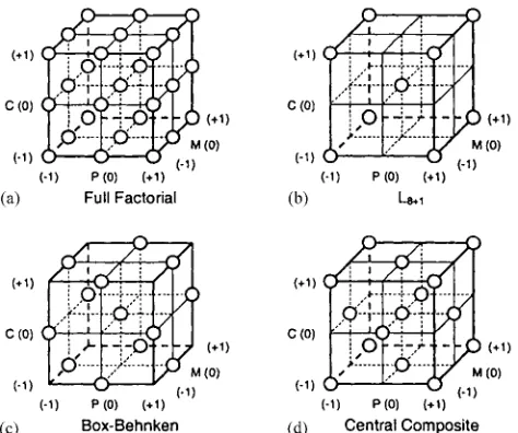
A full factorial experiment was used to investigate cost schedules over these three specific levels or settings of the parameters and was replicated five times using different random number seeds to facilitate the determination of real predictors—Figure 1a. A full factorial refers to the fact that every possible combination of the specific settings is used in

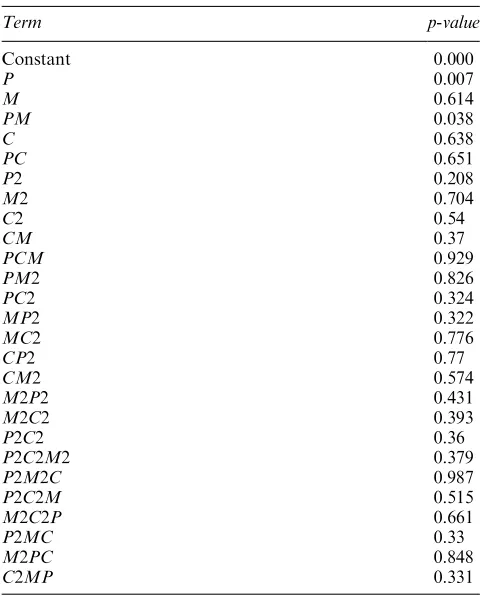
the set of trials. Thus, for three-factors (here the GA parameters) at three levels, we get 27 trials in total. In factorial designs, it is possible to estimateN1 terms for a plan involving N trials. A three-level factorial over three factors like this will provide us with a mathematical model or polynomial that has up to 26 terms, plus a constant that represents the effects on the response (here the cost) of the parameter settings in combination. This will include, where deemed necessary, quadratic terms as well as first-order ones, plus interaction terms that consider the changing effects on the response of one parameter as another is varied. Table 2 shows the full range of terms available from this three-level full factorial including the constant. The ‘P ’-values shown here indicate that factors P and M are considered important if all the terms are considered together in an analysis. In the table, a ‘2’ in the first column of terms indicates a quadratic term or quadratic component of a term.

These models can be quite comprehensive and provide a good approximation to reality over the whole range of the chosen settings, including combinations not chosen in the trials run, even in situations displaying considerable non-linearity. The results were analysed with a multiple regres-sion-based method known as ‘best subsets’. A fuller general

Table 1 Experimental parameter settings

Parameters with denoted coding Parameter settings and coded values

(1) (0) (þ1)

Populationgeneration combination size—P 20:60 40:30 60:20

Chance of crossover—C(%) 30 60 90

Chance of mutation—M(%) 2 10 18

description of the method is given in Draper and Smith,8 Montgomery9 but the essence is to look at all possible combinations of the potential terms within the mathematical model. Important terms are deemed to be significant if by adding them to the model there is significant improvement in the predictive capability of the mathematical model as discussed in a later section. Other methods are possible, such as ANOVA—the analysis of variance—or graphical meth-ods that are covered in later sections. In ANOVA, the terms are given the well-known ‘p’-values that display the probability of the term not being important. Traditionally, a term with ap-value of 0.05 or less is taken as important and thus retained in the model. This point is further discussed in later sections.

Parameters and associated effects found to be significant using ‘best subsets’ and sequential ANOVA wereP,Mand the interaction betweenPandM(PM). The results indicated that the crossover probabilityCis not significant within this application, across the region considered, which concords with results in Pongcharoen et al.4,5 _{None of the other} potential model terms were found to make a significant difference to the results. This paper assesses trying small subsets of the whole factorial to determine that a smaller design with fewer runs would have been sufficient to discover the same important parameters.

Fractional experimental design

A number of different smaller experimental designs were considered within this investigation including: a two-level fractional-factorial with one centre point (denotedL8þ1) in nine runs as described in Grove and Davis;10 a Box– Behnken design with 13 trials (see Box and Draper1), and, a central composite first described in Box and Wilson11with 15 trials—Figure 1. All are based on the relevant subset of the data from the full factorial using all five replicates. ‘Fractional’ indicates that the design is a fraction of a full factorial.

The L8þ1 experiment uses the extreme points on the vertices of the design plus a centre point, an extra trial run with all parameters set in the middle of their range, over the five replicates giving a total of 45 trials—Figure 1b. The results from this combination were then used to produce standardized coefficients (these are weighted in relation to the standard deviation associated with their estimation) as in Grove and Davis,10as well asT-values which are displayed within Figure 2. These results are interesting since they again suggest that the dominant predictor isP, however, the only other significant predictor, according to ANOVA isM, with thePM interaction and all other predictors being insignif-icant. In a screening experiment (a term used to denote that we are at the first stage of a set of trials and may add to them later) it should be borne in mind, however, that effects that appear at first sight to be too small by traditional standards (where terms with ap-value over 0.05 were excluded) may in fact be important, see for example Box and Liu.2In Sexton et al,12_{it is pointed out that effects with aP-value of 0.2 or} less should not be excluded in these initial stages. The reason for this is that in small screening designs the statistical power of the analysis, literally our ability to detect real effects, is reduced because of the smaller number of runs conducted. Thus, a larger p-value, traditionally attributed to insignif-icant effects, has to be viewed in relation to the amount of information available. A fuller discussion of this, in relation to the structure of GAs, is given in Poncharoenet al.13In the half-normal plot in Figure 2, that is basically a normal probability plot that is folded in half, the standardized coefficient10for the curvature (denoted curve) can also be seen to be small giving no indication of curvature on main effects within the design space. Details of the procedure used to determine the ‘curvature’ are also given in Grove and Davis.10This suggests that we do not need to determine the magnitude of the effect of the quadratic terms, and the current model is sufficient as a good predictor of the response. Of course, in our case we know this already from the full factorial results, but it is instructive that this smaller design gives similar results to our bigger experiment with all 27 trials. Previous investigations have, however, demon-strated that the test for curvature within a main effect may fail if the design space contains or surrounds a saddle point,14so some care has to be taken.

Table 2 p-values and terms for full ANOVA analysis of original full factorial

Term p-value

Constant 0.000

P 0.007

M 0.614

PM 0.038

C 0.638

PC 0.651

P2 0.208

M2 0.704

C2 0.54

CM 0.37

PCM 0.929

PM2 0.826

PC2 0.324

MP2 0.322

MC2 0.776

CP2 0.77

CM2 0.574

M2P2 0.431

M2C2 0.393

P2C2 0.36

P2C2M2 0.379

P2M2C 0.987

P2C2M 0.515

M2C2P 0.661

P2MC 0.33

M2PC 0.848

The design space was tested for saddle points within the PM plane, by examination of the PM plot based on the mathematical model (see Figure 5) and was discovered to be relatively flat and free from such phenomena. Thus, we can trust the fact that the ‘curve’ estimate is reliable in this case. Analysis of ‘best subsets’ (see Montgomery9or Hines and Montgomery15 for a fuller explanation by writers from an engineering background) was also tried in order to find the best regression equation based upon a number of standard criteria as shown in Table 3. In this table, column 1 shows the number of terms in the model on that row, the specific terms are listed by s in the last seven columns. The criteria are:

the coefficient of multiple determination, Rp2 which

represents the proportion of the sum of the squares deviation in the response variabley, about the predicted valuesyˆ, that can be attributed to the regression; the adjusted determination coefficient RR2_p, that accounts

for the number of predictors used in the model and the number of treatments within the experiment;

the square root of the mean squared error,s;

and, Mallow’sCpstatistic which is a measure of the total

mean square error for the regression model, compared to the estimate of background uncertainty, but adjusted forp.16

As the Rp2 criterion increases, so does the predictor’s

collective ability to predict the response, hence the largest value for Rp2generally represents the best model. However,

the coefficient of multiple determination rises as the number of predictors grows. The adjusted coefficient of determina-tion (RR2

p) is independent of the number of predictors in the

model and is consequently a more useful indicator thanRp2.

Increasing values ofRR2_prepresent increasingly better models. Mallow’sCpmay be used to estimate the relative amount of

bias, with less biased models having lower values for Cp,

which are usually close or equal to the number of predictors within the model. It can be seen from Table 3 (that gives the two best models for each number of terms in the model up to 5) for example that the model with onlyPMandPis not as good as the model withPandMmain effects. The results Figure 2 Half-normal plot and ANOVA for standardizedL8þ1coefficients.

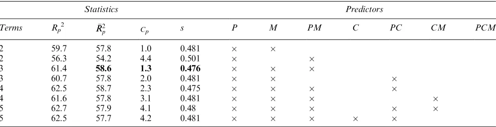
Table 3 Best subsets regression forL8þ1

Statistics Predictors

Terms Rp

2 R R2

p Cp s P M PM C PC CM PCM

2 59.7 57.8 1.0 0.481

2 56.3 54.2 4.4 0.501

3 61.4 58.6 1.30.476

3 60.7 57.8 2.0 0.481

4 62.5 58.7 2.3 0.475

4 61.6 57.8 3.1 0.481

5 62.7 57.9 4.1 0.48

suggest that a model including just P, M and the PM interaction is the ‘best’ one. No increase in predictive power or reduction in uncertainty in the statistical model can be achieved from adding more terms. The best model with four terms has almost identicalRp2,RR2p andsvalues and a higher Cp. We can rely on the model with three terms.

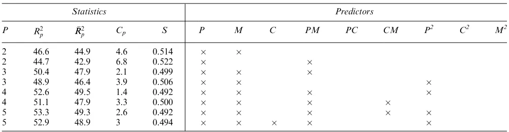
The central composite design is composed of a standard two-level factorial or fractional factorial design augmented with one or more centre points run in the middle of the design space, as in the design just discussed above, plus two extra runs per main predictor known as star points. The star points can be run in the centre of each ‘face’ of the cube portion of the design—Figure 1d. The idea of the star points is to enable estimates of the quadratic terms if the test for curvature suggests that this is necessary. Thus the CCD in this case is just theL8þ1 design with the addition of star points and thus not surprisingly gave similar results to the L8þ1. In fact, it is clear from the results above that inclusion of the star points would not provide better models. The Box–Behnken design is another quadratic design that does not contain an embedded factorial or fractional factorial matrix—Figure 1c. In this design, the treatment combina-tions are at the midpoints of the edges of the design space plus one at the centre. It is mostly used in situations where the most extreme conditions of the experimental space are difficult or impossible to run. The Box–Behnken design gave similar results, as shown in Table 4. We can see that the addition of the quadratic form of parameterPdoes improve the model slightly. As a rule of thumb, to justify the addition of another term to a model, a fall insshould be greater than the equivalent of the inverse of ‘the number of trials run minus 1 minus the number of parameters in the model’ (here 744¼70). So a fall of over 0.499/70¼0.00712 is required and so the addition ofP2does not really improve the model in this case.

Sequential experimentation

The idea of a sequential strategy is well suited to computer experimentation, there being no penalty from adding extra trial results at a later stage. In the industrial experimental

setting, we must take account of blocking or time effects and treat the results using split-plot analysis.9_{Here there are no} time effects, we can add extra results knowing that they will be identical to ones run under the same combination of factor settings at any time. Thus, the optimum strategy would be to run the minimum number of trials, observe the results, and if necessary add further trials as required. In this case, if the centre point results from theL8þ1had indicated the presence of curvature in a main effect, we could run the star points in order to estimate the quadratic effects that cause the curvature. Another tool used to assess regression models is the residual plot. This is simply the plot of the difference between observed values and model predictions for those observations, against various criteria. These plots would usually include; the order of experimentation, the factor settings and the fitted values of the model. In the case of computer experiments, the run plot is immaterial but if a pattern exists in the other types this may indicate the need for a missing term in the model. By the sequential use of these plots, and the model assessing criteria shown in Table 2, we can continue until a good model is selected. Figure 3 shows the fitted values against residuals for theL8þ1model and Figure 4 the mutation settings against the same residuals. No particular non-random patterns are visible although one possible outlier is present.

Table 4 Best subsets regression for Box–Behnken

Statistics Predictors

P R2

p RR2p Cp S P M C PM PC CM P

2

C2 M2

2 46.6 44.9 4.6 0.514

2 44.7 42.9 6.8 0.522

3 50.4 47.9 2.1 0.499

3 48.9 46.4 3.9 0.506

4 52.6 49.5 1.4 0.492

4 51.1 47.9 3.3 0.500

5 53.3 49.3 2.6 0.492

5 52.9 48.9 3 0.494

If the residuals had indicated a clear pattern, then we could have added the star points or the edge midpoints from the Box–Behnkin design. Clearly, such a strategy will lead to savings in time and computer resource in many cases. In the present case, running just the L8þ1 would have led to a saving of 66% in the time taken to run the original experiment. Cases with a greater number of factors can lead to many times this saving, see for example Poncharoen.13A sparse design, if considered prior to the original investiga-tion, could also have included the separate investigation of the population count and number of generations, rather than including these combined as a ratio as they were in this case. Other research suggests that mutation appears to be more useful than crossover for small population sizes;17 while crossover may be more useful than mutation for large population sizes.18

Follow up experimentation

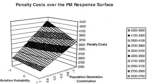
Having discovered the best settings for the parameters, in this case setting the population generation combination at

the high level (60–20) and setting the chance of mutation at the high level (18%) we can see that the experimenters had not yet found the optimum solution. Figure 5 shows a 3D response surface of the final model7 over the PM design space. The model was: Predicted total cost

d¼3380553P180Mþ149PM.

It can be seen that the optimum would appear to be somewhere off the plot at higher levels of the probability of mutation and higher populations. By adding a few more runs in the ‘direction of steepest descent’ which is easily determined,9 we could track smaller and smaller penalty costs until we found a design area that contained a minimum. The strategy would then be to run another small factorial experiment around the new minimum, possibly augmenting with star points if determined necessary, to find the definitive minimum. In the event, further work13showed that a better GA (with differently written mutation and crossover operators) existed so further work using this particular one has ceased. It should also be noted that crossover probabilities became important in the new GA, whereas here they were not. It should be noted further that the probability range for crossover is completely different than that for Mutation. We can only say that probabilities in the range of 0.3–0.9 make little difference to results, but a choice of, say, 0.1 may well make a difference, we cannot tell from these results.

Strategy for DOE-based computer program development

Establish the parameters or factors over which experi-ments will be conducted. These can be measured on categorical, ordinal or continuous scales. They should be able to be controlled (that is, can be set at particular levels) during the experiment, independently of the other factors. If this is not true, derived factors of these that can be set independently may be used, such as the ratio between two factors. Categories may be the type of coding, a program structure or a problem type. Include as many factors as possible.

Decide on the response to be optimized. This can also be measured on categorical, ordinal or continuous scales. This could also be a derived measure such as a ratio or sum.

Decide on the range of parameter settings. These should ideally be wide enough to cover factor levels that might show a discernable difference in the response. Typically, the highest and lowest possible, where a scale is available, are chosen.

Decide for each factor if a quadratic term may be likely to be needed. If so this will require three levels in the design, meaning at least a centre point.

Decide on an initial ‘screening’ design. This will mean choosing as few trials as possible that cover the design space over all the factors. This should be as sparse as Figure 4 Plot of absolute value of residual versus coded

probability settings for mutation.

possible and will typically have no fewer than (2N)þ1 trials forNfactors.

Run the screening design and analyse the results to produce an initial mathematical model.

Discard all unimportant factors and run further trials if the results are not clear or if the need for more complicated terms in the model is indicated.

Now search for the most optimum combination of factors, possibly moving outside the original range of factor settings and running more experiments.

Report the optimum model and use to demonstrate the best computer program.

Use the model as a benchmark against which to compare new programs and developments in future as these occur. Add new runs as necessary to include new factors as they surface.

Conclusions

This paper demonstrates how a sequential strategy using experimental design for investigating a GA would have resulted with significantly fewer experimental treatments than that performed within the actual investigations. The L8þ1 design demonstrated how similar conclusions would have been drawn with a more parsimonious initial design. Identical results to those obtained from the full design were also obtained using the central composite design. The overall conclusion is that a sparse experimental design would have sufficed in this case, however, additional experimental runs could have been conducted had the analysis indicated the need to do this or if the designer suspected the need to do so. Further experiments could be used to add to the experi-mental area once the direction of the optimum solution has been established. We have argued that computer experi-ments are an ideal use of DOE due to the lack of any experimental error that is usually experienced in real-life applications because of unplanned differences between experimental conditions. We have given a brief roadmap for the use of these designs and highly recommend a sequential strategy based on these designs in all such investigative work whatever the nature of the computer program being written.

References

1 Box GEP and Draper NR (1987).Empirical Model Building and

Response Surfaces. Wiley: New York.

2 Box GEP and Liu PT(1999). Statistics as a catalyst to learning by scientific method part I—an example.J Quality Technol31: 1–15.

3 Adams J, Balas E and Zawack D (1988). The shifting bottleneck procedure for job shop scheduling.Mngt Sci34: 391–401. 4 Pongcharoen P, Hicks C, Braiden PM, Stewardson DJ and

Metcalfe AV (2000). Using genetic algorithms for scheduling the production of capital goods. In: Grubbstro¨m RW and Hinterhurber HH (eds). Proceedings of the 11th International Working Seminar on Production Economics, February 21–25 Austria, Igls, Innsbruck, Austria.

5 Pongcharoen P, Hicks C and Braiden PM (2004). The development of bicriteria genetic algorithms for the finite capacity scheduling of complex products, with multiple levels of product structure.Eur J Opl Res152:215–225.

6 Goldberg DE (1989).Genetic Algorithms in Search, Optimisation and Machine Learning. Addison-Wesley: Reading, MA. 7 Todd D (1997).Multiple criteria genetic algorithms in

engineer-ing design and operation. PhD thesis, Engineering Design Centre, Department of Marine Technology, University of Newcastle upon Tyne.

8 Draper NR and Smith H (1966).Applied Regression Analysis.

Wiley: New York.

9 Montgomery DC (2001).Design and Analysis of Experiments,

5th edition. Wiley: New York.

10 Grove DM and Davis TP (1992). Engineering Quality &

Experimental Design. Longman: London.

11 Box GEP and Wilson KB (1951). On the experimental attainment of optimum conditions.J R Stat Soc13(1): 1–38. 12 Sexton CJ, Dunsmore W, Lewis SM, Please CP and Pitts G

(2000). Semi-controlled experiment plans for improved mechan-ical engineering designs.Proceedings of the Institute of Mechan-ical Engineers, Part B,J Eng Manuf214: pp 95–105.

13 Poncharoen P, Stewardson DJ, Hicks C and Braiden PM (2001). Applying designed experiments to optimise the perfor-mance of genetic algorithms used for scheduling complex products in the capital goods industry. J Appl Stat 28(3&4): 441–455.

14 Stewardson D, Porter D and Kelly T(2001). The dangers posed by saddle points, and other problems, when using Central Composite Designs.J Appl Stat28(3&4): 485–495.

15 Hines WW and Montgomery DC (1990). Probability and

Statistics in Engineering and Management Science. Wiley: New York, USA.

16 Mallows CL (1973). Some comments onCp.Technometrics15: 661–675.

17 Eshelman L (1995). Philips Laboratories, Briarcliff Manor, NY, USA, personal communication.

18 Spears WM and Anand VA (1991). A study of crossover operators in genetic programming. In: Ras ZW and Zemankova

M (eds). Proceedings of the International Symposium on

Methodologies for Intelligent Systems, Methodologies for In-telligent Systems. Volume 542. Springer-Verlag: Berlin, pp 409–418.