The Effect of Fishing on the Evolution
of North Sea Cod
Jessica Bridson
Submitted for
Degree of Doctor of Philosophy,
Department of Statistics and Modelling Science,
University of Strathclyde.
Young boy with two cod fish, Battle Harbour, Labrador ca. 1900
(PANL VA 21-18)
Copyright
c
The copyright of this thesis belongs to the author under the terms of the
United Kingdom Copyright Acts as qualified by the University of Strathclyde
Regulation 3.51. Due acknowledgment must always be made of the use of any
Abstract
With the recent collapses of many major fish stocks and North Sea cod
seeming to be the next on a long list, it has become apparent that our actions
have a great effect on fish populations. This thesis looks at how fishing can not
only have an immediate effect such as causing declines, but can also affect the
evolution of a stock.
A population model is built which is first examined for stability properties.
A comparison is also made of the model under fishing and when fishing is absent.
A measure of population fitness in terms of ability to invade other populations
is then established. This measure is used to examine the sensitivity of the model
to parameter values. This is also done for models which use different functions
to model life history in order to determine the importance of model choice.
Components of fishing mortality are considered with respect to their impact on
the stock, for both the main model and the alternate models. Finally, spatial
and seasonal considerations are added in a simple way to check if a single region
model can be trusted to model the whole of the North Sea.
It is found that although the model is sensitive to the choice of growth
function, generally growth has the most effect on population fitness. It is also
shown that the level of fishing has more impact on the fitness and yield of the
stock than the initial capture length. Thus, it is more important to reduce fishing
effort, than change aspects of the fishery such as mesh size in nets. Furthermore
the spatial model shows that the establishment of reservoirs, or no-fishing zones,
should be done carefully in order not to favour a decrease in growth rate of the
Acknowledgments
I would like to start by thanking the University of Strathclyde for making it
financially possible for me to study for this degree. I must also thank my two
supervisors. First Dr. S. Blythe, my original supervisor, for the many useful
ideas he suggested as well as his advice and practical help. I am also severely
indebted to Prof. W. Gurney, who became my supervisor for the writing up stage
of the thesis and has provided much needed advice, support and encouragement.
Special thanks are due to Craig, Colin, Shima and my parents who all proofread
parts of the thesis at various stages of completion. I would also like to thank Ram
Myers for encouraging my interest in fisheries modelling as an undergraduate
student.
It would be remiss of me to forget my colleagues in the department, who
dur-ing the three years have become friends. Their optimism and encouragement, as
well as their willingness to listen to my ponderings on cod, is much appreciated.
I also thank Craig for his love and understanding during the peaks and troughs
of writing up. Finally, I must thank my family who have always been a source
Contents
I
Introduction
1
1 The Life History of Cod in the North Sea 2
1.1 Cod and its Place in the World . . . 2
1.2 The North Sea . . . 4
1.3 The Life of a Cod . . . 6
1.4 The Recent Past . . . 10
2 A Modelling Background for Fish Stocks 13 2.1 Modelling Populations . . . 13
2.2 Stock Assessment Models . . . 16
2.2.1 Data Collection Methods . . . 18
2.2.2 Assessment Models . . . 22
3 Thesis Plan 26
II
Single Population Models
30
4 Construction of a Model 31 4.1 Creating a Single Population Model . . . 314.1.1 Age Structured Model . . . 31
4.1.2 Finding Equilibrium States . . . 33
4.2 Fitting Mortality Parameters . . . 35
4.2.1 Natural Mortality . . . 35
4.2.3 Fishing Mortality . . . 42
4.3 Fitting Parameters for Fertility . . . 44
4.3.1 Proportion Mature . . . 45
4.3.2 β . . . 47
4.3.3 K . . . 47
4.4 Models . . . 48
5 Behaviour of the Population 51 5.1 Stability of the Model . . . 52
5.1.1 Finding Stability Equations . . . 52
5.1.2 The Boundaries of Stability Behaviour . . . 54
5.2 Finding Stability in Complicated Models . . . 56
5.2.1 Fourier Transforms . . . 56
5.2.2 Fast Fourier Transforms . . . 57
5.2.3 Simulation Method . . . 60
5.3 Results and Robustness . . . 63
5.3.1 Results . . . 63
5.3.2 Robustness . . . 67
5.4 Summary . . . 70
5.4.1 An Unfished Population . . . 71
5.4.2 The Addition of Fishing . . . 72
5.4.3 Discussion . . . 72
III
Competing sub populations
80
6 Evolution through competing phenotypes 81 6.1 Introduction . . . 826.1.1 Clonal versus Genetic Models . . . 85
6.1.2 Different Methods of Examining at Evolution . . . 87
6.2 Competing Populations . . . 90
7 Finding the Best Fishing Policy 95
7.1 Introduction . . . 95
7.1.1 Methods of Sensitivity Analysis . . . 96
7.1.2 Introduction to Factorial Design . . . 98
7.1.3 Taguchi’s Design Method . . . 103
7.1.4 Examination of Sensitivity Method . . . 104
7.2 How Do Life History Parameters Affect Population Fitness? . . 106
7.2.1 Comparison of Full and Fractional Designs . . . 109
7.2.2 Implications for the North Sea Cod . . . 112
7.3 Robustness of Sensitivity Results . . . 116
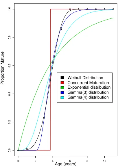
7.3.1 Alternate Functions for Proportion Mature . . . 116
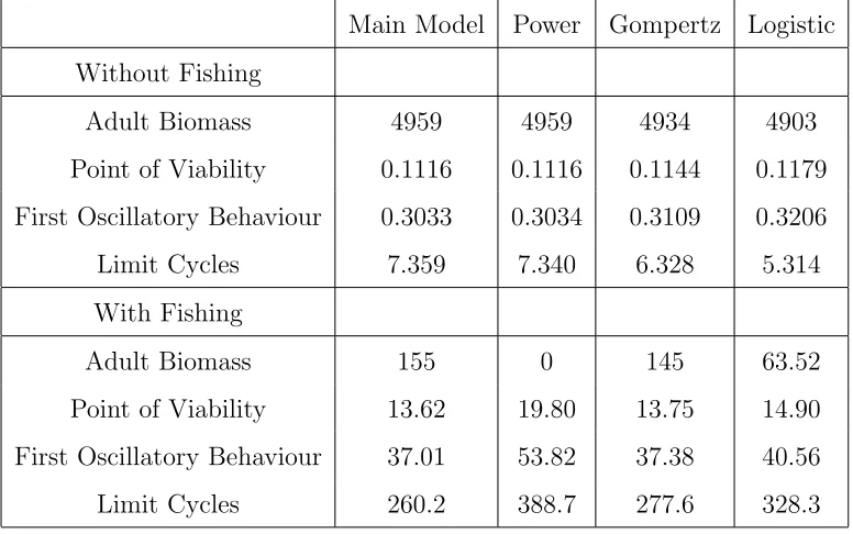
7.3.2 Alternate models for Growth . . . 121
7.3.3 Comparison with Results from Similar Work . . . 126
7.4 Reducing Fishing for Maximum Results . . . 127
7.4.1 Construction of Design . . . 127
7.4.2 Results . . . 129
7.4.3 Implications for the Fishery . . . 131
7.4.4 Alternate maturation models . . . 132
7.5 Conclusions . . . 133
8 Seasonal and Spatial Considerations 136 8.1 The Effect of Seasonal Reproduction . . . 136
8.1.1 Transfer Functions . . . 137
8.1.2 Simulation results . . . 139
8.2 The Effect of Migration . . . 143
8.2.1 Introduction to Spatial model . . . 143
8.2.2 Examination of Results of Simulations . . . 144
8.3 Discussion . . . 150
IV
Discussion and Conclusions
152
B Solver Programs 164
B.1 Constants Program . . . 166
B.2 Definition Program . . . 168
List of Tables
4.1 Natural Mortality at Age . . . 35
4.2 Defining Points for Fishing Mortality . . . 43
4.3 Fishing Mortality at Weight . . . 44
5.1 Equilibrium Values . . . 63
5.2 Stability Boundaries with Respect to Fertility (β) . . . 64
5.3 Equilibrium Adult Biomass under Different Maturation Schemes 68 5.4 Stability Boundaries for the Models under Different Growth Schemes 69 7.1 A Simple 2 Level Design . . . 99
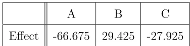
7.2 Effects of a 2 Level, 3 Factor Design . . . 99
7.3 A Simple 2 Level, 3 Factor Fractional Design . . . 100
7.4 Fractional Design Effects . . . 101
7.5 Alias Creation for Factor A . . . 102
7.6 Chosen Parameter Values for Sensitivity Analysis . . . 106
7.7 Grand Average Effects . . . 107
7.8 L27(313) Aliases . . . 110
7.9 Grand Average Effects for Fractional Designs . . . 111
7.10 Parameter Values for Alternate Proportion Mature Models . . . 117
7.11 Chosen Parameter Values for Alternate Growth Models . . . 122
7.12 Chosen Parameter Values for Sensitivity Analysis of Fishing Pa-rameters . . . 128
7.13 Grand Average Effects for Fishing Parameters . . . 129
List of Figures
1.1 North Sea Spawning Areas . . . 5
1.2 The Life Cycle of Cod . . . 7
1.3 Adult Biomass . . . 11
4.1 Natural Mortality Survival Curve . . . 36
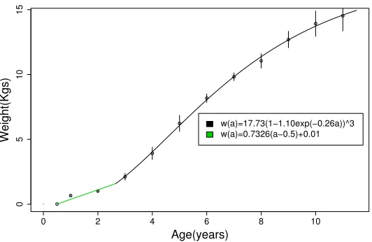
4.2 Weight at Age . . . 37
4.3 Comparison of Growth Curves for Young Cod . . . 40
4.4 Weight at Age under Different Models . . . 40
4.5 Natural Mortality at Weight . . . 41
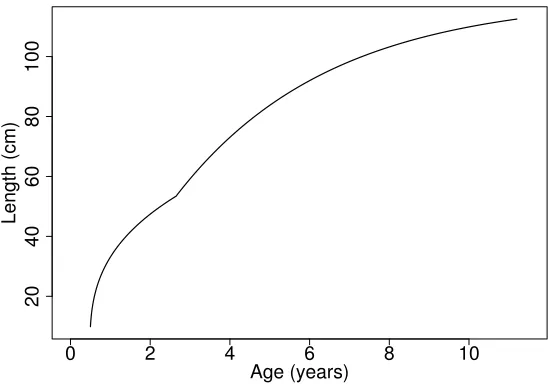
4.6 Length at Age . . . 42
4.7 Fishing Mortality at Length . . . 43
4.8 Survival Under Both Natural and Fishing Mortality . . . 45
4.9 Proportion Mature . . . 49
4.10 Approximations for Proportion Mature . . . 50
5.1 A Simple Exponential Function and its Fourier Transform . . . 59
5.2 FFT of an Exponential Function . . . 61
5.3 u(a) for the Unfished and Fished Models . . . 75
5.4 Behaviour at Different Fertility Values . . . 76
5.5 Behaviour at Different Fertility Values . . . 77
5.6 Stability Behavior forpy . . . 78
5.7 Stability Behavior forw∞ . . . 79
7.1 Average Responses of Life History Parameters . . . 108
7.3 Interaction Plots . . . 111
7.4 Equilibrium Plots . . . 113
7.5 Effect Plot for Model with No Fishing . . . 115
7.6 Effect Plot for Gamma(3) Maturation . . . 118
7.7 Effect Plot for First Alternate for Proportion Mature . . . 119
7.8 Effect Plot for Second Alternate for Proportion Mature . . . 120
7.9 Effect plot for Gamma(4) Maturation . . . 120
7.10 Effect Plot for Power Growth . . . 123
7.11 Effect Plot for Logistic Growth . . . 124
7.12 Effect Plot for Gompertz Growth . . . 124
7.13 Fishing Effect Plot . . . 130
7.14 Interaction Plots . . . 131
7.15 Plot of Effects of Fishing Parameters on Fitness in Model with Gamma(3) Maturation . . . 133
7.16 Plot of Effects on Fitness for Power Growth Model . . . 134
7.17 Plot of Effects on Fitness for Gompertz Growth Model . . . 134
7.18 Plot of Effects on Fitness for Logistic Growth Model . . . 135
8.1 Transfer Functions . . . 140
8.2 Simulation Plots . . . 142
8.3 Spatial Behaviour . . . 147
8.4 Spatial Behaviour . . . 148
8.5 Spatial Behaviour . . . 149
C.1 Interaction Plots . . . 177
C.2 Interaction Plots . . . 178
C.3 Gamma(3) Effect Plots . . . 179
C.4 Concurrent Maturation Effect Plots . . . 180
C.5 Exponential Effect Plots . . . 181
C.6 Gamma(4) Effect Plots . . . 182
C.7 The Effects of Life History Parameters . . . 183
C.9 The Effects of Life History Parameters . . . 185
Part I
Chapter 1
The Life History of Cod in the
North Sea
1.1
Cod and its Place in the World
Cod (Latin nameGadus morhua) is one of the most important fish species in the
world both historically and economically. The family of fish to which it belongs,
the Gadiformes or codfishes, is one of the three most utilized families in marine
fishing (Lindberg 1974). Other members of this family caught by world fisheries
are the haddock, pollock (also known as saithe), whiting, hake and Pacific cod.
In total 6 million tons of gadiform fish are caught each year and more than half
of this is Atlantic cod (Kurlansky 1997).
The cod is so popular due to its abundance and use as a food source. It
is the whitest of the white flesh fish, has virtually no fat (.3%) and very high
protein levels (18%), even in comparison to other fish (Kurlansky 1997). Almost
every body part is used or eaten, including the throat, cheeks, airbladder (also
used to make a clarifying agent and in some glues), roe, stomach, tripe, milt (or
sperm which is eaten in Iceland and Japan), bones which are softened and eaten
in Iceland, and the skin which is eaten in some places and also used to make
leather (Kurlansky 1997).
The cod fishery has a long history and has influenced many of the countries
is Newfoundland, an island province of Canada, which had battles waged for
its cod and was settled by fishermen needing land to dry their catch. At one
time the richest fishing grounds lay off its shores on the Grand Banks, and fish
were so plentiful that the Duke of Milan was told ‘the sea there is swarming
with fish, which can be taken not only with the net, but in baskets let down
with a stone’ (Harris 1998). The fish has had such an impact on the culture and
economic survival of the occupants, that the word ‘fish’ is synonymous with cod.
In the 1960’s onward, ships from around the world could be seen in harbours
and offshore, with countries such as Spain, Portugal and Russia playing major
roles in the development of the fishery.
However, tragically, in the 1980’s overfishing was to devastate the stocks
sur-rounding Newfoundland. A moratorium on fishing was finally declared in 1992,
which has still not been lifted in the northern waters, apart from the occasional
‘food fishery’ intended for individuals to fish only enough to provide cod for
their own tables. This collapse can be blamed almost completely on overfishing
(Myers, Barrowman, Hoenig, and Qu 1996), although at first other hypotheses
were made, such as seal predation or climate change. Hyperstability had a role
to play in the decline, with cod densities in certain locations increasing while
numbers decreased on the stock basis, resulting in misleading assessments of the
stocks (Rose and Kulka 1999). The stocks have reached such dire levels that it
has been recommended by Dr. K. Bell (a Memorial University of Newfoundland
fisheries ecologist) that cod should be added to Canada’s endangered species
list (Harris 1998), although they currently have only been listed as vulnerable.
There are also serious questions on whether the northern stocks will ever return,
as originally their return was forecast in 5 years, and 10 years later there still
seems no evidence that the stocks will ever reach their previous levels. This
return to former glory has been slower than predicted partly due to the low
fertility of the stock (Oosthuizen and Daan 1974).
The problem with drastic declines in numbers is unfortunately not restricted
to Newfoundland; in the late 80’s the Barents Sea stock also suffered a serious
the stock (Oosthuizen and Daan 1974) has seen this stock rebound to levels not
seen in 25 years (Harris 1998), and it is still, along with the Icelandic fishery,
one of the two most important fisheries of cod (http://www.fishbase.com). The
North Sea has also undergone declines, for instance in 1902 the British found
that its cod stocks had been depleted (Kurlansky 1997). In 2001, it was decided
that a decline in stocks was such that it required a moratorium from February
to April (for certain areas) while drastic quota cuts have been implemented in
recent years.
The economic power of cod is clearly demonstrated by the fact it is one of
the few species that wars have been fought over. To some extent, as previously
mentioned, the desire for cod has led to battles over Newfoundland waters. A
more recent example, which is certainly remembered in Britain, is the Icelandic
cod wars. In the late 1950’s till early 70’s, Iceland expanded its fishing limits
on other countries to 12, then 50 and finally 200 miles offshore (Kurlansky
1997). These increases in limits prompted what have become known as the ‘cod
wars’. Although no lives were lost, Icelandic boats did cut the trawls of vessels
inside the limits with 84 trawlers losing their nets in a year of conflict in 1971
(Kurlansky 1997). Shots were fired during the wars, and on May 26th, 1973 a
hole was blown in the hull of a British trawler (Kurlansky 1997).
In the rest of this chapter, we will first examine the area of interest to this
thesis, the North Sea, and then look at the life cycle of a cod in this body of
water. We will then continue by examining the current state of the North Sea
cod stock and the problems the area is experiencing.
1.2
The North Sea
The North Sea is a body of water surrounded by Europe: on the west side
the United Kingdom, to the north east Norway, with Denmark, Germany, the
Netherlands and Belgium all having coast along its edge. It is a fairly shallow
basin, varying in depth from 30 to 200 meters (Brander 1994). Its surface area
Figure 1.1: The North Sea : The black lines show the limits of what is considered
as the North Sea. Speckled areas are spawning grounds used by cod. The map
was drawn with the help of http://odin.dep.no/md/html/conf/map and the Atlas
of the seas around the British Isles(1981)
through the northern North Sea (Brander 1994).
Different ages of cod are found in different places in the North Sea. Age 1
cod are most common along the coast of the Netherlands and northeast England
as well as in the German Bight, as are age 2 cod, although they also are found
in the Northern North Sea. Age 3 cod are mainly in the northern North Sea,
while age 4 cod and older are scarce throughout (Brander 1994). Spawning areas
are scattered across the North Sea as shown in figure 1.1, where they are the
speckled regions.
The North Sea can be divided into six distinct regions using hydrography
have, however, found no clear sub-stocks which are identifiable within these
regions (Brander 1994). Hence, in terms of fisheries assessment, the North Sea
is normally considered as a single region, sometimes also including the areas
between Sweden and Denmark, known as the Skaggerak and Kattegat.
1.3
The Life of a Cod
The life cycle of cod has several different stages (figure 1.2). Cod start as eggs,
progress through a juvenile stage which switches level in the ocean, and finally
reach maturity. The timing of this life-cycle differs according to region, and
the first age at maturity in a stock can range from 2 years to 7 years depending
on which region the stock inhabits(http://www.fishbase.org). As such, although
the general life history is the same from stock to stock, the differences in duration
of life stages means that the reaction of the stocks to fishing pressure can be
quite different.
The eggs are extremely small (approximately 1.4 mm (R. Myers, Stock
and Recruitment data base, http://www.fish.dal.ca/ myers/welcome.html)), and
float on the surface drifting with the current. Cod eggs are spawned between
January and April, with latitude affecting the peak time of spawning: for
in-stance, the Southern Bight peaks in February while the northern North Sea peak
in spawning is in March (Brander 1994; Daan 1978). There is limited spawning
in the autumn, but the main spawning season is during the spring (Brander
1994; Anonymous 1981). Spawning takes place in many different areas of the
North Sea and figure 1.1 shows where these areas are found. It should be
men-tioned that due to the similarity between haddock and cod eggs, it is not known
exactly where the cod spawn as both spawn at similar times (Daan 1978; Fox,
O’Brien, Dickey-Collas, and Nash 2000).
In order to develop normally the sea temperature to which the eggs are
exposed should be between 1.5 and 12 degrees Celsius (Thompson and Riley
1981), so years with exceptional sea temperatures can have an effect on the
Figure 1.2: The Life Cycle of Cod. This includes 5 life stages with
all cod becoming adults by the age of 6 years (Background image from
hatching (Heesen and Rijnsdorp 1989). Mortality is assumed to be caused mainly
by predation, as eggs supply such an easily obtainable food source, and several
species eat cod eggs. Herring have been cited as one of the main predators, and
the ‘gadoid outburst’ has been suggested to have been caused by a decline in
the herring stocks. However, Daan found herring eat only between 0.04% and
0.19% of eggs in the North Sea (Daan, Rijnsdorp, and Overbeeke 1985).
Once cod hatch they become larvae, although according to Brander (1994)
very little is known about this stage. This is due to two main reasons. During
the early stages of life, the rates of production and mortality of eggs and larvae
change rapidly making accurate modelling of this age range very difficult.
Sec-ondly there is no assessment of the catching efficiency of gear for fish of this age,
preventing good estimates from being made of the percentage caught (Sundby,
Bjorke, Soldad, and Olsen 1989). The combination of these two properties makes
drawing any conclusions from data on this age risky.
The egg sac does not disappear immediately upon hatching. Larvae live off
the egg sac for about 6 days, by which point it has been completely resorbed
(Brander 1994), although some larvae do begin to feed at sizes as small as 3.1
mm (Last 1978). After this stage larvae fend for themselves, and many will
perish by drifting into areas where food of a suitable size is scarce (Northern
Cod Science Project). They feed on phytoplankton and zooplankton, principally
eating nauplii and copepodites of calanoid copepods, with prey being determined
by the mouth size of the larvae (Last 1978; Thompson and Riley 1981). At this
stage mortality is still very high, and as many as 99.9% of fish die in the first 4
months of life(Northern Cod Science Project).
The next stage of life, that of juveniles, can be divided into two parts. A
pelagic life stage where fish live towards the top of the water column, and a
demersal life stage where fish settle towards the bottom. The pelagic stage
differs in duration between areas, being very short or perhaps nonexistent for
fish in the southern North Sea (Brander 1994). In other areas, particularly
off the coast of Jutland and in the central North Sea, this stage may last as
juveniles are found in shallow areas of the North Sea (Daan 1978). Robb and
Hislop concluded that competition for food is not great among these juveniles
(Robb and Hislop 1981). Cod this age eat mainly copepods until they are 3
centimeters in length, after which their diet is dominated by fish, the largest
component being Norway Pout, another gadoid fish (Robb and Hislop 1981).
By 6 months the juveniles have settled to the bottom layer of the ocean,
where rocks and weeds give cover to avoid predation, a major consideration for
the smallest fish. They are eaten by several other gadoid fish, including cod,
whiting, and saithe. At this stage they consume mainly crustaceans although
as their size increases fish become a more important component in their diet
(Daan 1973). It has been found that juvenile cod (mainly under 15 cm) make a
significant contribution to the diet of other cod, being 10% of the diet by weight
in the northern North Sea, while only 1% to 2% in the southern North Sea
(Daan 1973). My model will start with this life stage, avoiding the difficulty of
modelling the extremely high mortality experienced in the previous 3 life stages.
The final stage of a cod’s life is adulthood, although very few of the eggs
spawned will actually produce adults. Some cod become mature as young as
age two, but some cod in the North Sea do not mature until they are six years old.
(Oosthuizen and Daan 1974). Males mature earlier than females (Oosthuizen
and Daan 1974), although in my model this is not considered as there are not
separate models for the two sexes. As adults, the key role of the fish is to
reproduce, with older female fish spawning more eggs over a longer time period
than their younger counterparts (Harris 1998). The current levels of fishing,
however, prevent there being many of these older female fish, and most fish will
die before maturation. When stocks are being rebuilt, it is the re-establishment
of a healthy population of these older female fish, which will vastly increase the
rate of recovery. Fish migrate to spawn, with spawning grounds generally to the
south of feeding areas (Brander 1994), although these migrations are relatively
short. Adult cod mainly eat fish, including many species used by commercial
fisheries including young cod. Mature cod are relatively large fish, and as such
1.4
The Recent Past
Historically, the North Sea has not been the most abundant producer of cod;
in the 16th through 19th centuries Dutch fishermen sailed to Iceland for cod
rather than staying on the North Sea (Brander 1994). There was, however, a
large increase in numbers of cod in the 1960’s, a phenomenon seen in many
gadoid populations, and given the name the ‘gadoid outburst’ (Holden 1981).
This rise in numbers is thought to possibly be linked with the decrease, due to
overfishing, of the herring population (Daan, Rijnsdorp, and Overbeeke 1985).
For a while afterward, spawning stock biomass (or adult biomass) fluctuated,
but from 1981 there has been a steady decrease in the population, and biomass
is now at the same levels as before the 1960’s (Brander 1994). In fact, levels are
so low that the spawning stock biomass is now considered to be well below the
safe biological limit of 150 000 tonnes for the stock (Brander 1994). This level
(known as MBAL orBpa) is believed to be the spawning biomass below which the
probability of low levels of recruitment increases. Another reference point used
in fisheries management is Blim, the lowest value of spawning biomass observed
for the population. This value has been set at 70000 tonnes for the North Sea
cod stock (ICES 2002). There is great concern for the stock as spawning biomass
has hovered around this value for all of the 1990’s.
The current situation in the North Sea is definitely worrying. In 2001 forty
thousand square miles of ocean were closed to fishing from February to April
in order to protect the spawning stock, and the European Union council of
ministers has agreed to the lowest total allowable catch (TAC) ever. This quota
cut is necessary as there is a lack of large spawning fish due to the long term
rise in fishing effort and a decrease in recruiting young cod (Christensen 2001).
A fisheries collapse in the North Sea has been predicted for many years, and
during the last ten years fishermen have barely managed to catch their quotas,
with ever smaller fish being caught (Christensen 2001). Hopefully, the actions
of the European Union in closing the grounds and cutting catches will have the
Figure 1.3: The Decline of Adult Biomass in the North Sea (Data from ICES
(2002)):Plots of both adult biomass and recruitment are given. They clearly show
that the population levels have dropped in the 1990’s
1970 1980 1990 2000
50
100
150
200
250
Year
Adult Biomass (thousand tonnes)
1970 1980 1990 2000
200
400
600
800
Year
in the North Sea and the cod stocks off Newfoundland. There is some argument,
however, over the level to which it can be hoped the stock will return. It may be
unrealistic to expect a return to the levels of the 1960’s and 1970’s which were
Chapter 2
A Modelling Background for
Fish Stocks
This chapter will examine modelling as a tool for learning about fish populations.
It will start by discussing how models can be used to solve problems raised about
populations, and then mention the main models used for fisheries assessment in
the North Sea. Although these models are not used in this thesis, they are
crucial to virtually any work done for populations, as parameters are frequently
set using information which has come from such stock assessments.
An important aspect of fisheries assessment is data collection. The different
methods are discussed, in order to give a sense of the complexities involved in
making an assessment. Upon consideration of the difficulties involved with
as-sessing ocean stocks, much respect is gained for the difficulties faced by both
fisheries scientists and managers in trying to assess stocks and set sensible
guide-lines for fishing.
2.1
Modelling Populations
The first question is why should populations be modelled? The simple answer
is that models are a tool to help us understand the complexities of the world
around us. A good model should be simple to use and understand, give results
the field of interest. Models, by necessity, are a simplification of the world. It is
impossible to quantify the effect of every part of the environment. Such a model
would take so long to create and use that it would not be practical to build.
The model would also produce unreliable results as it is not clear how to model
many environmental factors and the interactions between factors which affect a
population. Hence, models tend to choose a few key factors which are felt to be
essential to finding the answer that is sought. These factors will often include
ranges of environmental factors grouped into one parameter and thought of as a
noise or an environmental effect. Some of the defining characteristics of models
and how they will be treated in this thesis will now be discussed.
One key aspect of modelling is to decide which questions the model will
be answering. For example, is the interest in modelling an entire ecosystem,
a sub-community of the ecosystem, a particular species, or how an individual
copes with living in its environment. In each case the model produced will
be substantially different. This thesis will focus on cod at the species level.
Therefore, although we recognize that the population consists of a number of
individuals whose weight and maturation are modelled, a general maturation
and growth scheme for the population as a whole shall be used. An
alterna-tive approach would be to assume that individuals follow a general growth and
maturation scheme, but that for each individual this scheme differs slightly. By
tracking individuals the picture of the general population can be constructed.
This method, often referred to as individual based modelling, has the advantage
that it is a more accurate depiction of the population, as not all individuals will
grow identically. It was felt, however, that as we are interested in examining the
impact of fishing on the population as a whole, this was a complication to the
model which was unnecessary. Furthermore, the entire ecosystem will not be
modelled. It will be assumed that food is distributed so that all cod have equal
supplies, mortality affects the population as a whole and does not have a spatial
term (although in chapter 8 this assumption will be changed), and that human
fishing is not affecting food supply for the cod at the same time as it affects
still allowing us to examine the impact of fishing on the population.
The next key point is how time should be modelled. Fishery models
fre-quently make use of discrete time models, where time is considered as moving
forward in chunks, often using a spacing of a year. Simulations of the
popula-tion are then easy and data collected for the growth, maturity and mortality
of the stock can be used without having to make assumptions of the functions
underlying the life history. In this thesis, however, a continuous time model will
be used, as growth and fertility are modelled as gradually occurring processes
for the population, as opposed to processes which occur in sudden leaps and
bounds. Although this is more realistic, the impact the function chosen for a
certain aspect of life history will have on any results must be considered. Using
a continuous time model implies that when simulations are run, a different
dis-crete time step model shall be used, however, by using small time steps for the
simulations, differences in results can be minimized.
It is also important to recognize that random events have an impact on
the behaviour of populations. There are two ways to approach this random
behaviour when modelling. The first, deterministic modelling, ignores the
ran-dom behaviour and instead is aimed at finding the main trend. It necessarily
assumes that the random behaviour is insignificant in comparison to the
un-derlying trend. When the results of such a model are compared to what is
seen in the environment, it is expected that model results will not be an exact
replica of the real world. Instead it is hoped that, on average, a deterministic
model is accurate. This requires that environmental fluctuations will not take
a regular pattern with respect to the deterministic solution, and secondly, that
these fluctuations will not be so large that they hide the deterministic effects.
Another approach to treating random effects, is stochastic modelling. Instead
of the model giving, for instance, the decrease in population over a time period,
the stochastic model gives a probability of a certain decrease in population over
the time period. As such stochastic modelling can sometimes be thought of like
an experiment, where several realizations can be averaged to give an idea of the
world situation can change, and if enough realisations are run there should be
some which resemble what has happened in the environment. The main trend
found by a stochastic model may be the same as the trend found by a
determin-istic model, but there exist situations where there is little resemblance between
the two. I have chosen to use a deterministic model, as it was felt to be the
simpler of the two methods and would let me solve problems numerically as well
as through simulation.
A final consideration is the inclusion of spatial dynamics into a model. I shall
begin by not including spatial considerations, assuming instead that the North
Sea is uniform in its distribution of food, mortality, and numbers and weight of
fish. However in chapter 8 a glimpse of what can happen when the North Sea
is divided into different spatial regions shall be given. Only two regions shall be
used, but even with such a small change, the complexity of the model increases
as now immigration and migration have a role to play.
These are some of the main considerations when building a model. It must
then be determined which individual aspects should be included, for example,
numbers, weight, length, maturity, condition, toxicity levels, or a combination
of factors in the model. These same basic tools can build models to answer
a variety of questions about a population, such as the effect of temperature,
sunlight, pollution, food levels or fishing.
2.2
Stock Assessment Models
One of the initial questions frequently asked in fisheries is ‘how many fish are
there and how many can we safely catch?’. Since it has been realized that
the oceans have their limits, and are not an inexhaustible source of fish, several
different models for stocks have been used. In this section several of these models
shall be introduced.
There is no standard model which is used for all fisheries assessment. For
instance a survey done by the National Marine Fisheries Service in the United
age-structured models, 28.3% with abundance models, 8.0% with production models,
6.1 % with stock reduction models and further stocks were either not assessed,
or assessed using professional judgement or other means (Committee on Fish
Stock Assessment Methods et al. 1998). In section 2.2.2 I shall discuss in detail
the age-structured models which are generally used for North Sea cod (such as
extended survivor analysis), however I note that there are many other models
which are found to be appropriate for other regions and species.
We start with a rather obvious question, but one that must be answered,
‘Why should fish stocks be assessed?’. The clear answer is that whatever the
state of a fishery, there are always inherent problems or dilemmas which must
be solved. For developed fisheries these are quite obvious questions, such as
‘how many fish can be caught next year safely?’ or ‘is the fishery reducing the
population to unfishable levels?’. For underdeveloped fisheries, questions such
as ‘How much can this stock yield?’ and ‘How can we best plan to exploit the
fishery?’ are important (Gulland 1983).
The second question is how accurately can populations be assessed.
Accu-racy of fish assessments is indeed a serious problem. In the collapses of both
North Sea herring and Newfoundland cod stocks, assessments did not show that
the populations were crashing until stock levels had already decreased
consider-ably (Hilborn and Walters 1992). This was compounded in both cases by the
management of the stock. In the case of North Sea herring quota cuts were
recommended in 1970, yet in 1974 managers of the fishery agreed to a TAC
which was larger than the total population (Hilborn and Walters 1992). There
are many worries about the catch data which is frequently used in analysis, as
many scientists are skeptical of the ability to detect stock trends using such data
(Hilborn and Walters 1992). It is also known that such data can have serious
biases. Some stocks can become easier to catch at low numbers due to increased
shoaling. If old values are used to estimate the ability to catch a stock this can
have profound consequences. Catch records may also ignore discards and in the
worst case scenario have been falsified. There are further worries as most stock
other populations. The North Sea is one area in which multi-species analysis
is used periodically, however, Daan (quoted in Hilborn and Walters 1992) has
pointed out that such models are very data intensive and that the tools for doing
multi-species models properly don’t exist as of yet. A final difficulty with
assess-ing fish populations is that population numbers are difficult to assess, in that
although some acoustic and sonar methods are used, fish cannot be counted or
observed as easily as animals living on the surface. Instead they must generally
be caught in order for assessments to be made, adding the extra difficulty of
assessing how well equipment catches the population and if it catches a
repre-sentative sample.
A quick run down of different data collection methods will now be given,
followed by a brief summary of different assessment models.
2.2.1
Data Collection Methods
There are four main ways to collect data, by using commercial fishery data,
research vessel surveys, tagging data and lab experiments. Each of these different
methods has different relative costs, advantages, and uses for fishery scientists.
Upon examining the different methods of data collection it becomes apparent
that this is a major area of consideration in fisheries assessment. Without good
data on which to base models, there is little hope that accurate assessments of
populations can be achieved or that any model of population behaviour can be
accurate.
Commercial Fishery Data
Commercial fishery data has the advantage that it examines exactly how
fisher-men are interacting with stocks, and if unbiased and truthfully reported will give
an accurate picture of the mortality inflicted on a stock. In terms of ecosystem
management, commercial data is grossly biased. Fishermen will only target fish
which are financially rewarding, and hence not give an accurate idea of stock
levels for all species in the oceans (Gulland 1988). The most important data
observa-tions on the amount of fishing and corresponding catch, and the size and ages
included in the catch (Gulland 1988).
Catch and effort data is best collected by on-board observers. These
ob-servers can give accurate accounts of when and how the fishery is conducted,
as well as giving information on bycatch, discarding and violations of
conserva-tion measures (Hilborn and Walters 1992; Committee on Fish Stock Assessment
Methods et al. 1998). All of this information is very difficult to obtain without
having an impartial observer on board boats. These observers can also take
information on the specifics of the catch, such as species, age and sex
distribu-tion caught. However, the problem with obtaining data in this manner is that
observers are expensive, in that they must be well trained before being used
and sometimes constitute (in terms of the economics of a fishing boat) a useless
member of the crew. Careful assumptions must be made when extrapolating
observer data to the full fishing fleet as it can be expected that observers will
affect fishing practices in many cases, rules are more likely to be strictly followed
and gear maintained properly.
Another method for using commercial data is on shore observations of catch.
During the sale of fish catches, records are kept on size and weight as a matter of
course, and these records can be used by scientists to assess the catch.
Further-more there are programs which sample catches as they come in for age and sex
distribution (Committee on Fish Stock Assessment Methods et al. 1998). Of
course such methods are not capable of assessing discards of undesirable species
or fish too young to be caught in legal mesh sizes, and hence lose some of the
data an observer can provide. This collection method is, however, much cheaper.
A third method used in commercial fisheries is examination of logbooks of
fishermen. For instance, in Australian trawl fisheries, notes on the start and end
locations and the size of the catch are made in the logbook, allowing spatial maps
of the population to be created (Hilborn and Walters 1992). Unfortunately, this
method rarely gives information on age and species caught, and depends on the
fishermen giving an accurate report of what has happened at sea. Once again
tends to produce the most accurate data.
Research Survey Data
The second method of data collection is by using research surveys. These surveys
are very expensive as a boat must either be owned or hired to do the survey,
and is unable to catch fish in a competitive commercial manner. The main
advantage of such surveys is that they can use good sampling designs and study
the ability of different gear to catch fish. Furthermore, as they are used for
research purposes, not commercial purposes, an accurate picture can be built
of the proportions of different species in the oceans. Three different ways of
obtaining data from research surveys shall now be discussed.
For some populations visual observation can be adequate, if the species
sur-faces frequently. Assumptions must then of course be made about frequency of
surfacing and also observer reliability (Hilborn and Walters 1992) in order to
estimate numbers. This method of observation will only provide data on
num-bers and is unlikely to allow observers to collect any data on sex or age of the
population. As such it is rarely used.
Electronic and hydro-acoustic surveys can also be performed. The advantage
being that this method does not harm the fish. In order to collect good data,
however, certain problems do need to be solved. For instance, the strength of the
signal received from targets must be calibrated with the number of individuals,
and there is also the problem of species identification (Hilborn and Walters
1992). Many aspects of the population will not be measured in such a survey,
including individual size, sex and age of the species monitored. Such methods
have been used for tracking migrations of populations, and discovering where
in the water column populations live at particular times of the day, year or
migratory route.
The most frequent use of research vessel surveys is using commercial fishing
gear in imitation of the commercial fishery. Whatever is caught can be fully
documented, for all important characteristics such as weight, length, age, sex
inter-est, rather than targeting only areas where fish are known to congregate as in
commercial fisheries. The exact configuration of the gear will also be known,
allowing for an accurate assessment of its performance. The only assumption
which needs to be made is the proportion of fish captured by the gear and its
selectivity (Hilborn and Walters 1992). This can be assessed by using a
combi-nation of gears (for instance with different mesh sizes) to evaluate the ability of
the larger mesh size to catch fish.
Tagging Data
The third method of data collection which is in standard use is tagging. This
is done by putting a tag on the fish through a fin or embedded in flesh. This
method allows for the survival, movement, mortality and abundance of fish to be
estimated by using the recovered tags to estimate how the population lives. Some
tags send radio or acoustic signals, so that the fish can be tracked continuously
by boats on the surface. This is generally used to examine daily migrations,
changes in depth, or eating patterns. Other types of tags must be recaptured in
order to allow assessments of migration or movement, and likely abundances and
mortalities to be estimated. Recovery of tags can be difficult sometimes, as many
will not be returned when the fish is caught. Thus estimates need to be made
for tags not recovered as to how many are due to tag loss, natural mortality, and
lack of reporting. Further assumptions must then be made on whether the tags
have any effect on the fish carrying them. As such it is often difficult to obtain
accurate results through tagging, or even sometimes to estimate how accurate
results are (Gulland 1988).
Laboratory Experiments
A final method of data collection which can be useful to the fisheries scientist
is laboratory experimentation. It has both the weakness and strength that
conditions can be strictly controlled. This is an advantage in that life-history
parameters such as growth can be measured accurately knowing the true age
laboratory results can not be expected to translate fully to life in the wild where
conditions alter from hour to hour and region to region. Furthermore, there are
size limits on how large and deep a laboratory tank can be, making it difficult
to truly replicate a wild environment. The difficulty of observation in the ocean,
makes this a very attractive method for gaining data on virtually every aspect
of life-history and behaviour.
2.2.2
Assessment Models
The models for assessment, which depend on these data, will now be introduced.
Assessment models are frequently based mainly on commercial data, however
other types of data, such as tagging data are essential for their information
on natural mortality. Tests are also being made of models using only research
survey data to see if there is any advantage in excluding fisheries data and if
these models could act as a check on the normal assessments (Cook 1995).
There are several different assessment models used for commercial fisheries.
The type of fish being examined and the method of fishing affect which model
will be used. I will examine in detail only two models, as these are the models
which are used most often for North Sea cod.
Many other simple assessment models do exist. Stock-recruitment models
are perhaps the most simple as they are generally used for stocks where age
effects are not important (Hilborn and Walters 1992). Thus the spawning stock
is thought of as a single group which reproduces in the same manner for all
ages. Hence this model is frequently used for species which spawn only once in
their lifetime. Tretyak (1999) has expanded this model to use age-classes for
North-Eastern Arctic cod.
Production models are another type of model which do not require that the
population is broken into age-classes. Under this model the manager sets a
level of biomass which should be maintained and which, by setting the catch
to be less than the growth and new recruits contribution to the population
biomass, should either remain constant or increase. This is frequently used by
estimates of management parameters than age structured models, as shown
by Ludwig and Walters(cited in Hilborn and Walters (1992)). Furthermore for
populations which are difficult to age, such as many tropical stocks (Jones 1984),
these methods are the best available.
However, when fish reproduce over a long lifetime and change how well they
spawn with age, a model which breaks the population into age-classes can often
provide better advice. In the North Sea two such models, XSA and MSVPA are
used.
Age-Structure Models
The first age-structure model we shall discuss assesses a single species, and is
often known by the name virtual population analysis (VPA), although there are
many more models, similar in approach, such as ADAPT, CAGEAN and Stock
Synthesis (Committee on Fish Stock Assessment Methods et al. 1998). The
extended survival analysis model (XSA) is the version which is currently used
in the North Sea. Each cohort or year class of fish, is treated separately under
these models. The basic premise used is that
Nt,a =Nt+1,a+1eM +Ct,ae
M
2 (2.1)
where Nt,a is the number of fish of age a in year t, M is natural mortality and
Ct,a is the catch of age a fish in the year t (Hilborn and Walters 1992; Myers,
Hutchings, and Barrowman 1997). Generally this method is used to estimate
backwards in time, and thus, only estimates numbers for cohorts which are no
longer in the population. Also, fish are only considered once they reach the
age of entry into the fishery, avoiding tracking the population for ages where
natural mortality is high. In order to estimate forwards, natural mortality rates
are assumed to be constant and assumptions are made about the fishing
mor-tality on the oldest age class (Hilborn and Walters 1992; Myers, Hutchings, and
Barrowman 1997). One way to do this is to assume
whereF is fishing mortality,Eis effort andqis catchability. Parameter estimates are made for q from previous cohorts and then adjusted using data on cohorts which have not completed their life cycle. For the North Sea an XSA iteration
begins with an initial guess at how many fish will survive past the oldest age
group for which records are kept. A standard VPA is then used and catchability
and an exponent linking numbers to the CPUE index of abundance estimated. A
series of iterations is then repeated until convergence is obtained for the estimates
of sizes of cohorts (for more information see Lassen and Medley (2001)).
Although VPA has many advantages, in that it can use full age data, it is
not a perfect assessment model. For instance, collecting the age data required
can be very expensive (Committee on Fish Stock Assessment Methods et al.
1998). The heavy dependence of this assessment method on catch data can
cause problems when catchability of a stock or age class changes with declining
stock numbers. This is a particular danger for clupeoid stocks, which have a
tendency to increase their catchability when stock numbers are low (Hilborn and
Walters 1992). Further difficulties become apparent if there is immigration into
a population or two stocks are assessed as one. The VPA model could show a
decrease in fishing mortality while one of the substocks was completely fished
out (Daan 1991). Similarly misreported landings can have a serious effect on
this method (as well as the methods previously mentioned) as this can lead to
numbers or fishing mortality be estimated incorrectly (Patterson 1996). As a
final note, it is important that aging is done accurately. If a certain percentage of
fish are thought to be mis-aged every year, then if a weak cohort is preceded by
a strong cohort, it is possible that numbers in the weak cohort are overestimated
(Hilborn and Walters 1992).
A further extension to the VPA modelling idea has been implemented in the
North Sea, that of Multi-Species Virtual Population Analysis (or MSVPA).
Un-der this method, stock assessments for more than one population are made by
separating mortality into three components: fishing mortality, mortality inflicted
by other cohorts included in the analysis, and natural mortality not otherwise
inter-actions between stocks, for instance giving a possible answer to the question of
whether one stock will increase if another is fished down, the quantity of data
required for an assessment is overwhelming. For each age class of each species
considered, stomach data must be found in order to estimate predation rates on
the species and age classes in the model. Only the computer advances of the
last few years have meant that such a model can be used. Daan’s message that
we ‘don’t really have the tools for multi-species analysis though single species
analysis is inadequate’ perhaps best summarizes the current situation (Hilborn
Chapter 3
Thesis Plan
The main aim of this thesis is to examine the impact fishing has on a population.
As cod is fished heavily in the North Sea, fishing is one of the most important
factors in the natural selection of cod. If it is possible to ensure that the yield
obtained from the fishery is sustainable in the short term (or on the ecological
time scale), it would be even more valuable to show that it is sustainable on the
evolutionary time scale. Thus we wish to discover if the results of the high level
of fishing now, will be a population in a hundred or two hundred years which is
unfishable, due to the decreased size or fertility of the population, or if there will
be relatively little effect. Although of interest from a modelling point of view, if
the impact of fishing is not felt within at most 500 years, it may not be worth
changing fishing practices, as environmental changes may swamp such an effect.
Knowing what pressures fishing can have on a population, can also help us
to understand what may happen in such environmental changes. For example,
if water temperature was to change such that fish grew more slowly and fishing
favored fish which grew quickly, this would be an indication that the
environ-mental change would have a serious effect on the fishery. If this was the case,
it would be worth lowering the level of fishing in order to give the population
some resiliency to environmental change.
If it is found through modelling that we can expect fishing to have a large
impact on the population it should then be considered when fisheries assessments
maturity schedule incorporated into fisheries assessments should be updated on
a regular basis, as fishing is likely to decrease size and age at maturity. Blythe
and Stokes (1991) find that there has indeed been a pressure on North Sea cod
to decrease size at maturity, further supporting Dr. Rochet’s calls for diligence
in assuring maturity ogives used are accurate. Their work demonstrates clearly
that we cannot expect fish stocks to remain stationary, they will react to the
pressures that we exert, and in assessing stock levels we should always remember
this.
The model in this thesis is strongly based on the model of Blythe and Stokes
(1991) and works to expand the complexity of their model. They assume that
all fish become adults at the same time, ageτ, where as the model in this thesis assumes a gradual change in proportion mature over a span of six years. It shall
be shown that a model allowing a gradual increase in proportion mature will also
favor changes in the life history parameters which decrease the age at maturity.
Another difference between the two models is that I have only modelled from age
six months upwards as I wished to avoid trying to model the life stages where
natural mortality is extremely high and changeable. The results found are quite
similar to the result found in Stokes and Blythe (1991) where they discovered
that harvest levels are now high enough to cause pressure for the weight at first
maturity to decrease.
The impact of finding that fishing is having a serious effect on growth and
maturity of cod could be important. If such effects are likely to become apparent
in the short term, it is certainly of consideration whether fishing practices should
be changed in order to lessen these effects. Assessing the importance of different
elements of fishing mortality is crucial, we shall try to do this by looking at three
different aspects of the fishing curve namely: the initial age of fishing, the peak
age for fishing mortality, and the overall level of mortality. If it is possible to
assess which of these factors is most important, it is possible to advise fishery
managers on how pressure on the stocks should best be reduced.
Cod is currently caught in a mixed fishery with a species which is much
are about 23 centimeters at maturity, about a third of the size of a cod at their
average age at maturity of four years (Alverson, Freeborg, Murawski, and Pope
1994). However the current mesh size catches fish at about size 30 centimeters,
with the legal limit for cod being 35 centimeters, obviously these sizes being far
too small as most cod are not yet mature at this age. Ideally cod would not be
caught until an age where a significant percentage of the population had been
given the opportunity to spawn at least once (Alverson et al. 1994), in order to
ensure that there was a resistance to extinction built into the population. It has
been shown that if a fished population has a sufficiently high maximum annual
reproductive rate and a policy of fishing was followed such that all fish were
allowed to spawn at least once, then fishing mortality could be increased to any
level without causing the population to become extinct (Myers and Mertz 1998).
If the initial size of capture is the most important determinant of the pressure
on the stock, then obviously the mesh size with which fisheries are practiced
should be increased so that only older cod are caught. This is a controversial
issue however, with Norway already advocating such an increase, while countries
such as Britain which catch large numbers of whiting resisting such an increase
due to the decrease the whiting catch would experience (Oliver 2001).
If it is found that the peak age of capture should be changed, i.e. the shape
of the fishing curve, then different measures are called for. This could be done
by examining selectivity of gear and trying to change the amount of each type
of gear used in the fishery, or by changing such things as mesh size in nets.
Lowering the overall level of fishing would perhaps be the easiest change to
make, as this could be changed by reducing quotas and effort in the North Sea,
or using less efficient methods for catching fish.
As a result, I will look at not only which life history parameters are likely
to change under current levels of fishing, but also which fishing parameters are
most likely to relieve such pressure if altered. I shall start by creating a model for
a single population and examining its stability properties, establishing whether
the population is viable in the long-term, and the type of behavior exhibited.
examine competition. A measure of fitness will then be found, enabling the two
populations to be compared in their ability to cope with the environment. In
chapter 7 I will look at a sensitivity analysis of the model which will help answer
the two main questions posed in this thesis. Finally I shall examine the effect
of two more additions to the model. First reproduction will be changed to a
seasonable variable, to see if this will have a noticeable effect on the population.
Secondly a very simple spatial model will be introduced to check if changes in
Part II
Chapter 4
Construction of a Model
4.1
Creating a Single Population Model
4.1.1
Age Structured Model
In this chapter I shall build the model which will be the basis for all work in
this thesis. The thesis characterizes a deterministic model for North sea cod and
hence the lack of goodness of fit tests in this chapter does not detract from the
usefulness of the model. Fertility and mortality have been modelled as depending
on age (and for later chapters size), rather than using blanket values across the
whole population. Growth and maturation are modelled as continuous processes
rather than as step functions as in many fisheries models.
After some consideration a standard model was adopted, the
McKendrick-von Foerster equation as described in Ecological Dynamics (Gurney and Nisbet
1998). The notation of Gurney and Nisbet will be used in the following
discus-sion.
This model is built by assuming that f(a, t) is a continuous age distribution of the number of age a fish at time t of the population, having the property that f(a, t)da is the number of individuals at time t that are in the age range
is given by
∂f(a, t)
∂t =−
∂f(a, t)
∂a −δ(a, t)f(a, t) (4.1)
where ∂f(a, t)/∂a is the change in f(a, t) with respect to age and δ(a, t)f(a, t) gives the mortality rate at time t. This model assumes that all cod which join the population at the same time grow in exactly the same manner. An
unrealistic simplification, but one that was felt necessary to avoid complications
which would make analytic work with the model impossible.
Clearly there must also be a mechanism for adding fish to the population and
as the model is of a closed population, this mechanism is the birth rate. Fish will
only be modelled from age six months, thus there is a six month delay term in
reproduction. Fish younger than this live in a different ocean layer (Anonymous
1981), and thus experience a different environment making it sensible to separate
out this group. Furthermore, mortality rates for very young fish and eggs are
extremely high and changeable due to natural causes making them difficult to
model as mentioned in chapter 1. As the production of fish obviously depends
on the population numbers and fertility of the population this leads to
f(0.5, t) = R(t) =
Z ∞
0.5 B(a, t−0.5)f(a, t−0.5)da (4.2) where B(a, t−0.5) is the production of half year old fish.
A changing environment is not used for the first part of this thesis, thus
mortality can be assumed to be independent of time. Hence the probability
that a fish will survive to age a (S(a)) is simply
S(a) =exp
Z a
0.5−δ(x)dx
(4.3)
and f(a, t) can be calculated for any age using R(t) and S(a) as
f(a, t) =S(a)R(t−a).
Notice that this now means using equation 4.2, the Lotka renewal equation
(Gurney and Nisbet 1998)
f(0.5, t) =R(t) =
Z ∞
holds true.
Now that the model form has been established, the two key components,
mortality and fertility, will be examined. The functions for both will be fitted in
sections 4.2 and 4.3. The mortality function is divided into two parts, natural
mortality and fishing mortality. Fishing mortality is defined as the mortality
imposed by human fishing, while natural mortality includes all other mortality
such as predation by birds, mammals and other fish, cannibalism, and death
due to human causes other than fishing. All fish are assumed to die by age 50
in the case of a population with no fishing and age 25 in a fished population as
survival rates are essentially zero for these ages (as will be seen in section 4.2).
The fertility function at age a and time t is
B(a, t) =βc(t)w(a)p(a) (4.5)
where β is the production parameter, c(t) is the competition function, w(a) is the weight at age, and p(a) is the proportion mature. Notice that by using the proportion mature in the fertility function, the average fertility at age is
used as mature and non mature fish are not separated into different groups.
The competition function c(t) gives a limit on how successful breeding is, and has the form c(t) = exp(−A/K) where A is the adult biomass and K is a limiting factor. The form of the competition function ensures that at very high
population levels fertility is low, possibly as there is higher mortality of very
young fish due to crowding and increased predation. This competition function
does not lower fertility at low population levels. Weight is included in the
fertility function as the number of eggs produced by fish is a linear function of
body weight (Oosthuizen and Daan 1974), hence fertility can be expected to rise
with body weight.
4.1.2
Finding Equilibrium States
The equilibrium values of a population provide important information. For any
real population there is always an equilibrium value of zero, such that if this
labelled the trivial equilibrium of the population, as it is obvious that if there are
no fish in the population there can obviously be no fish in the future, unless they
migrate into the area from another region. Furthermore, if the only nontrivial
equilibrium values are negative, it is a clear indication that the population is not
viable, and will in a matter of time become extinct. Hence, the next step is to
find the general form of the equilibrium for the population, under the assumption
that mortality and fertility are time independent.
If the population is assumed to be at equilibrium then
R⋆ =
Z ∞
0.5 B
⋆(a)S⋆(a)R⋆da (4.6)
and canceling R⋆ gives the renewal condition
1 =
Z ∞
0.5 B
⋆(a)S⋆(a)da. (4.7)
The fertility B from equation 4.5 is now substituted into equation 4.7 to give 1 =
Z ∞
0.5 βp(a)w(a)c
⋆S⋆(a)da (4.8)
hence
1
c⋆ =
Z ∞
0.5 βp(a)w(a)S
⋆(a)da. (4.9)
Using the form of the competition function,
e(A⋆/K)=
Z ∞
0.5 βp(a)w(a)S
⋆(a)da (4.10)
then
A⋆ =Kln
Z ∞
0.5 βp(a)w(a)S
⋆(a)da (4.11)
giving an easy way to calculate the equilibrium adult biomass. Using equation
4.6 it is seen that
R⋆ =βc⋆
Z ∞
0.5 p(a)w(a)S
⋆(a)R⋆da. (4.12)
But as adult biomass is simply
A⋆ =
Z ∞
0.5 p(a)w(a)S
⋆(a)R⋆da (4.13)
this gives
R⋆ =βe−A⋆/K
4.2
Fitting Mortality Parameters
As mentioned in section 4.1 mortality has been divided into two different
compo-nents. This is a natural thing to do in fisheries, mainly as one type of mortality
is uncontrollable (natural mortality) while the second (fishing mortality)
de-pends purely on the actions of fishermen, and is governed by the regulations
and quotas set by fisheries scientists and governments. Discard mortality, which
includes mortality caused by unwanted fish (due to age, size, species etc) being
caught during the fishery and thrown back, has not been specifically included.
Such mortality is difficult to estimate (Alverson, Freeborg, Murawski, and Pope
1994) and it is certainly possible that mortality rates are underestimated,
espe-cially for young fish.
4.2.1
Natural Mortality
The data for natural mortality comes from Cook (1998) and was given at age
as in the following table 4.1. These are standard natural mortality estimates for
the North Sea which can be found in many other papers.
Table 4.1: Natural Mortality at Age
Age 0.5-2 2-3 3-4 4+
Mortality 0.8 0.35 0.25 0.2
The corresponding survival curve, when considering natural mortality alone
(figure 4.1), shows that by age 20 very few fish will still be alive. This is what we
would expect the survival curve for the North Sea to look like if the population
were not fished.
The form of natural mortality has been changed in part 3 of the thesis when
more than one population is under consideration. For a single population having
natural mortality depend on age as opposed to size causes no problems as weight
is a function of age. However, as soon as a second population is introduced there