Rochester Institute of Technology
RIT Scholar Works
Theses Thesis/Dissertation Collections
11-1-2008
Multi-object decision making for supplier selection
in outsourcing
Pushpen K. Mohile
Follow this and additional works at:http://scholarworks.rit.edu/theses
This Thesis is brought to you for free and open access by the Thesis/Dissertation Collections at RIT Scholar Works. It has been accepted for inclusion in Theses by an authorized administrator of RIT Scholar Works. For more information, please [email protected].
Recommended Citation
MULTI-OBJECTIVE DECISION MAKING FOR
SUPPLIER SELECTION IN OUTSOURCING
Pushpen K. Mohile
B.E. (Production Engineering)
University of Mumbai
Thesis submitted in partial fulfillment of the requirements for the degree of
Master of Science in the Department of Industrial and Systems Engineering
in the Kate Gleason College of Engineering of the Rochester Institute of
Technology
KATE GLEASON COLLEGE OF ENGINEERING ROCHESTER INSTITUTE OF TECHNOLOGY
ROCHESTER, NEW YORK
CERTFICATE OF APPROVAL
________________________________________________________________________
MASTER OF SCIENCE DEGREE THESIS
________________________________________________________________________
The M.S. Degree thesis of Pushpen K. Mohile has been examined and approved by the thesis
committee as satisfactory for the thesis requirement for the Master of Science degree.
--- Dr. Sudhakar Paidy
--- Dr. Panchapakesan Venkataraman
Dedicated to
My Beloved Late Poppa
Kirit S. Mohile
Kirit S. Mohile
Kirit S. Mohile
Kirit S. Mohile
My Mommy
Nilam K. Mohile
Nilam K. Mohile
Nilam K. Mohile
Nilam K. Mohile
My Sister
ABSTRACT
ACKNOWLEDGEMENT
The successful completion of this thesis work would not have been possible without the help and guidance from a number of individuals.
First and foremost, I would like to thank Dr. Sudhakar Paidy for his significant support and care during my tenure of thesis study under him. I would like to thank him for all his guidance and advice which helped me develop my skills and knowledge in the areas of Supply Chain and Operations Research.
My special thanks to my two committee members, Dr. Marcos Esterman and Dr. Panchapakesan Venkataraman for their helpful comments and encouragement.
I would also like to thank all the staff members of the Industrial and Systems Engineering Department for their direct or indirect support during my tenure of thesis study.
TABLE OF CONTENTS
CHAPTER PAGE
NUMBER
1. Introduction 1 – 4
2. Supply Chain Management
2.1. Overview of Supply Chain Management 2.2. Challenges in Supply Chain Management
2.3. Supplier Selection in Supply Chain Management
5 – 11
6 7 11
3. Literature Review
3.1. Overview 3.2. Description
3.2.1 Multi-objective methods’ application in any field of study
3.2.2 Multi-objective methods’ application in Supply Chain field
3.2.3 Multi-objective methods’ application in “Supplier Selection”
12 – 20
13 14-20
15
17
19
4. Problem Statement 21 – 24
5. Criteria selection and justification 25 – 29
6. Multi Attribute Decision Making
6.1. Introduction
6.2. MADM application in this thesis study
30 – 34
7. Multi Objective Decision Making methods and examples
7.1. Introduction
7.2. Weighted Objective method 7.3. Goal Programming method 7.4. Evolutionary Algorithm method 7.5. STEM method
35 – 65
36 43 49 57 64
8. A Representative Supplier Selection Problem 66 – 72
9. A Heuristic Multi-Objective Methodology for Supplier Selection Problem
9.1. Overview
9.2. Description & Implementation
9.2.1. PHASE I: Evolutionary Approach 9.2.2. PHASE II: Goal Programming Approach
9.2.3. PHASE III: Progressive Articulation – STEM Approach
73 – 94
74 75-94
76 81 84
10.Conclusion 95 – 98
11.Appendix 1 – Literature Search Tables 104 – 109
12.Appendix 2 – Hardee Toy Example solved using STEM method 110 – 117
13.Appendix 3 – Important terms used in Thesis 118 – 120
LIST OF FIGURES
FIGURE PAGE
NUMBER
Figure 2.1: Basic Supply Chain Process 6
Figure 2.2: Series of links and shared processes between suppliers and customers
7
Figure 2.3: An Extended Supply Chain 8
Figure 2.4: Bullwhip Effect 9
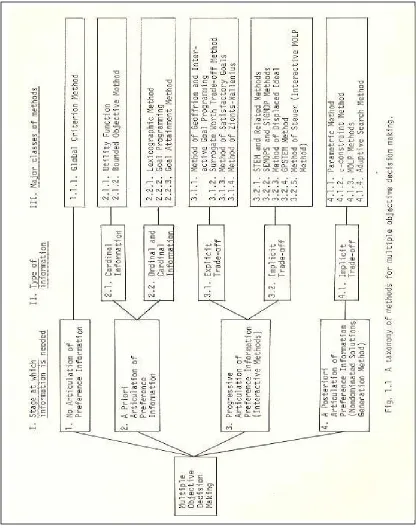
Figure 7.1: Taxonomy of Multi-objective Decision Making Methods
LIST OF TABLES
TABLE PAGE
NUMBER
Table 6.1 33
Table 7.1 45
Table 7.2 52
Table 7.3 59
Table 7.4 65
Table 8.1 68
Table 8.2 68
Table 8.3 70
Table 9.1 77
Table 9.2 78
Table 9.3 83
CHAPTER 1
1. INTRODUCTION
A supply chain is the system of organizations, people, technology, activities, information, and resources involved in moving a product or service from supplier to customer (Wikipedia). Supply chains can be defined as
real world systems that transform raw materials and resources into end
products that are consumed by the consumers. Supply chains encompass a
series of steps that add value through time, place, and material
transformation. Each manufacturer or distributor has some subset of the
supply chain that it must manage and run profitably and efficiently to survive
and grow. (Pinto)
The main and basic challenges in the supply chain are to plan a strategy to manage the resources and meet the demands, to select the suppliers that will deliver the goods and services that are required to build the product, to manufacture the product, to deliver the product to the customers and to make an arrangement for return of the product for servicing through customers, if there is any fault in the product.
future needs. “Some suppliers that meet some selection criteria may fail in some other criteria” (Wadhwa and Ravindran 3726). For example, the supplier selected may meet the “price” criteria but the company might have to compensate on the quality of the product and lead time. Selection of suppliers depends on various different criteria. Some criteria are quantitative such as “price of the product,” “lead-time for delivery,” “transportation cost,” etc., whereas some like “reputation of the supplier,” “cultural barrier,” “risk,” etc., are qualitative. No single methodology appears to be dominant in solving the supplier selection problem. In this study multi-objective decision making methodologies are applied to select the suppliers by optimizing various criteria (objectives) and a heuristic methodology is developed to find a suitable solution (final supplier(s)).
The basics of the supply chain and the extended supply chain which includes the challenges faced in supply chain management are discussed in Chapter 2, “Supply Chain Management.” Various areas of supply chain management and multi-objective optimization were reviewed and are presented in Chapter 3, “Literature Review.” Following the literature search, a supplier selection problem was selected for the thesis and is stated in Chapter 4, “Problem Statement.” Supplier selection depends on various criteria. Hence, criteria used for the supplier selection in the real world industries and by various authors, were studied and some of the important criteria were selected, as discussed in Chapter 5, “Criteria Selection & Justification.”
synthesized and stated along with its data, objectives, and the constraints in Chapter 8, “A Representative Supplier Selection Problem.”
CHAPTER 2
2. SUPPLY CHAIN MANAGEMENT
2.1 Overview of Supply Chain Management
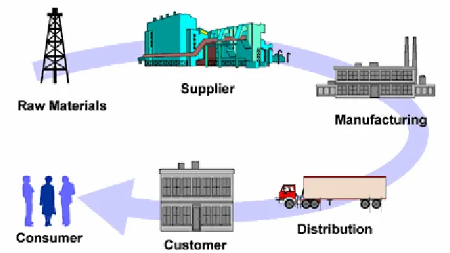
A supply chain is a series of links and shared processes that exist between suppliers and customers.
Figure
2.1: Basic Supply Chain Process
A supply chain is a network of facilities and distribution options that performs the tasks of procurement of materials, transformation of these materials into intermediate and finished products, and distribution of these finished products to the consumers (Ganeshan and Harrison).
Supply chain management is the act of optimizing all activities throughout the supply chain, so that products and services are supplied to the consumers in the right quantity, to the right location, at the right time and at optimal cost (Clarkston).
Suppliers Manufacturer
(value addition activity)
Customers
2.2 Challenges in Supply Chain Management
[image:17.612.154.476.284.465.2]These links and processes involve all activities from acquisition of raw material to delivery of the finished goods to the end user / consumer. Raw material enters into a manufacturing organization via a supply system and is transformed into finished goods. The finished goods are then supplied to consumers through a distribution system. Generally, several companies are linked together in this process, each adding value to the product as it moves through the supply chain (Clarkston) (Figure 2.2).
Figure 2.2: Series of links and shared processes between suppliers and customers
Source: Strahan, Bruce, and Art Van Bodegraven. Logistics vs. The Supply Chain. The Progress Group: White Papers. The Progress Group, Inc., 2004. Web. 10 Mar
2007 <http://theprogressgroup.com/publications/wp2_logs.html>.
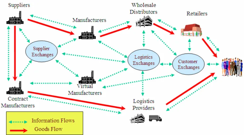
to many suppliers and consumers resulting in a complex extended supply chain (Figures 2.3).
Figure 2.3: An Extended Supply Chain
Source: Bauer, Michael-CSC Consulting and AMR Research. “E-Business: The Strategic Impact on Supply Chain and Logistics.” e-Business:_The Best Document Search Engine!. N.p. 2001. Web. 10 June 2008
<http://www.seeeach.com/doc/90560_e-Business:>.
The following are the five basic tasks for Supply Chain Management:
1. Plan: A strategy needs to be decided for managing resources, meeting demands and production.
4. Deliver: Coordinate receipt of orders from customers, develop a network of warehouses, and pick carriers to get products to customers and set-up an invoicing system to receive payments.
5. Return: Create a network to receive defective and excess products back from customers and support customers who have problems with the delivered products.
Challenges faced while managing the supply chain:
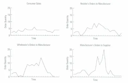
[image:19.612.110.522.366.635.2]Traditional supply chain management assumed that information needs to be shared only with the next point of contact in a supply chain. But this resulted in a Bullwhip effect which means small changes in consumer demand can result in large variations in orders placed upstream (Figure 2.4).
Figure 2.4: Bullwhip effect
2.3 Supplier Selection in Supply Chain Management
CHAPTER 3
3. LITERATURE REVIEW
3.1 Overview
Initially, the literature search focused on the general topic “Multi-Objective Optimization.” As mentioned by recent authors, “supply chain problems are complex and difficult to solve” (Pinto) and since multi-objective optimization methods are capable of solving such complex problems, the literature search later concentrated on “Application of Multi-Objective methods in Supply Chain area.” Through the wide literature review, it seemed that “Application of Multi-Objective methods in Supplier Selection” was in its infancy state. Hence, the literature search narrowed down to a topic, “Application of Multi-Objective methods in Supplier Selection.”
3.2 Description
The literature search in this research study focused on two major areas; “multi-objective methods” and “supplier selection in outsourcing.” The diversity of problems solved using the multi-objective methodology provides a backdrop for addressing the most challenging problem of the supply chain management: Supplier Selection.
3.2.1 Multi-objective methods application in any field of study
Initially general applications of multi-objective methods were studied. There are numerous topics/ areas under which multi-objective optimization studies have been done.
1. Varshney and Rao in their paper “Multi-Objective Crop Planning” use the linear goal programming method to optimize three objectives “to maximize irrigated crop area, to maximize net benefits and to maximize crop production” with “ total land water and crop area fertilizer” as its constraints and “hectares of land used per crop” as the decision variable.
2. Huang, Tian and Zuo in their paper “Multi-Objective Optimization of Three-Stage Spur Gear Reduction” use the interactive physical programming method to optimize three objectives “to minimize volume, to minimize surface fatigue and to maximize load carrying capacity” with “tooth bending fatigue failure, shaft torsional stress, face width interference and tooth number” as its constraints and “core hardness, face width, tooth numbers and diameter of the shaft” as the decision variables.
3. Oliveira, Volpi and Sanquetta in their paper “Multi-Objective programming in Brazilian Forest” use the goal programming method to optimize six objectives “to maximize wood harvest, to maximize number of tourists, to maximize the pasture (creation of buffalos), to minimize number of employees, to maximize the diversity of flora and to maximize the diversity of fauna” with “total land and forest area” as its constraints and “area used for timber, ervamate, leaves, pasture and tourism” as the decision variables.
protein-compound couple’s Van Der Waal’s & electrostatic energy of interaction and to maximize shape complementarities” with “computer specifications, population size and number of generations” as its constraints and “docking configurations (output complex of drug)” as the decision variables.
5. Weber, Charles and Lisa in their paper “Supplier Selection using Multi-Objective Programming” use the decision support system approach (compromise) to optimize three objectives “to minimize price, to maximize quality and to minimize late orders” with “number of units required, number of suppliers required to fulfill demand, quantity of late deliveries and quality restriction” as its constraints and “quantities ordered” as the decision variable.
3.2.2 Multi-objective methods application in Supply Chain field
Further, the search concentrated on the area of “multi-objective optimization in supply chain networks”:
1. Belgasmi, Said and Ghedira in their paper “Evolutionary Multi-Objective Optimization of the Multi-Location Transshipment” use the strength pareto evolutionary algorithm (SPEA2) method to optimize three objectives “to minimize total expected cost, to maximize fill rate and to minimize expected transshipment lead time” with “quantities shipped cannot be more than those available at store and quantities shipped cannot be more than unmet demand at store” as its constraints and “order quantities” as the decision variable.
2. Pinto in her paper “Supply Chain Optimization using Multi-Objective Evolutionary Algorithm” use the non-dominated sorting genetic algorithm-II (NSGA-II) method to optimize five objectives “to minimize total operating cost, to minimize manufacturing cost, to maximize profit, to maximize revenue and to minimize transportation cost” with “plant capacity, supplier capacity, inventory balancing constraints for respective components and total cost” as its constraints and “number of components shipped from plants to supplier, number of products shipped from plants to customer zones and inventory of components at plants” as the decision variables.
3. Mumford in her research “Multi-Objective Optimization for Green Logistics” uses “building multi-objective optimization decision support tools for strategic and operational SCM, with a special focus on environmental issues” as its objective.
cost, to minimize variable cost and to minimize volume flexibility” with “supplier capacity, production requirement, plant capacity, production capacity, throughput capacity, each customer zone assigned to one distribution center, products shipped are equal to products available at plants and total shipments are equal to demand requirements” as its constraints and “quantity of products produced in plants, products shipped from plants to distribution center, products shipped from suppliers to plants and cost” as the decision variables.
The problems within the research work mentioned above are:
1. In the weighted objective method, the decision maker needs to give the prior information about the importance of each objective to the analyst. The analyst can give weight to the objectives based on the information provided to him by the decision maker and optimize the resulting single objective.
2. Similarly, in the goal programming method, the decision maker needs to give the prior information to the analyst about the order in which the goals need to be achieved. The resulting problem is solved via a series of single objective problems (Hwang et al. 56).
3. A considerable number of evolutionary algorithms have been proposed in the last few years. Comparative studies have shown that amongst all the evolutionary algorithms created, the Strength Pareto Evolutionary Algorithm (SPEA2) and the Non-dominated Sorting Genetic Algorithm (NSGA-II) show the best performance (Belgasmi et al. 11). But in higher dimensional spaces, SPEA2 seems to have advantages over NSGA-II (Belgasmi et al. 11).
3.2.3 Multi-objective methods application in “Supplier Selection”
As one can see from the literature search, numerous articles have been written and researched on the topics “general multi-objective optimization technique” and “multi-objective optimization in supply chain management” but less research has been done on the topic “multi-objective optimization in supplier selection.”
Hence, the search narrowed down to “multi-objective methods used for supplier selection in outsourcing.”
1. Thaver and Wilcock in the problem “Identification of Overseas Vendor Selection Criteria used by Canadian Apparel Buyers” use a nine-point scale ranking system to optimize criteria “price, quality, willingness to negotiate prices, lead time for delivery, time for quotation, communication system, quantity required, technical expertise, merchandise fashionability, financial position, export quota, long-term commitment, economic stability in country, registered to quality program, processing EDI, registered to ISO 9000” and select the suppliers.
The subject identified in this paper is one in which there are too many questions and very few answers.
2. “The Outsourcing Institute’s Annual Survey of Outsourcing End Users,” article states, “price, commitment to quality, additional value-added capability, scope of resources, location, existing relationship, cultural match, reputation, flexible contract terms” as criteria for supplier selection.
and linear” as its constraints and “product quantity, binary variables for supplier and price level” as the decision variables.
Wadhwa and Ravindran have made suggestions in their paper that risk quantification and global supplier selection is gaining much importance in the real business world, which can be an extension to their work.
CHAPTER 4
4. PROBLEM STATEMENT
Outsourcing is defined as purchasing ongoing services and parts from an outside company that a company currently provides, or most organizations normally provide for themselves (Wadhwa and Ravindran 3725). Outsourcing is “paying another company to provide you with a service or product that you would otherwise have your own employees conduct” (Anthony). Many large organizations are outsourcing those activities which are not either cost efficient if done in-house or are not core to their businesses (Wadhwa and Ravindran 3725). Outsourcing the activity also means that the work is distributed and hence the time-to-market the final product can be reduced.
Recently, outsourcing has become the prime focus of the company (Wadhwa and Ravindran 3725). Cost reduction is not the only criteria for outsourcing but the ability to focus on core competencies is also an important criteria. Many companies are now evaluating, supply chain procurement and the logistics as the candidates for outsourcing. Various reasons for outsourcing are (Wadhwa and Ravindran 3726):
In many cases the third party can provide procurement services more efficiently. Outsourcing can provide access to specialized technology and operational platforms.
1. Outsourcing can help reduce the staffing levels.
2. The advancement in technologies has made procurement a very specialized service.
In the Outsourcing Institute’s Annual Survey of Outsourcing End Users (The Outsourcing Institute Membership), the reasons for outsourcing are stated as:
3. Gain access to world-class facilities 4. Free internal resources for other purposes 5. Accelerate the reengineering benefits 6. Make capital funds available
7. Share risks 8. Cash Infusion
A survey carried out by the Aberdeen group found that more than 83% of the organizations engaged in outsourcing achieved significant decrease in the purchasing cost, more than 73% of the industries found reduction in transaction cost and 60% were able to reduce sourcing and procurement cycles (Wadhwa and Ravindran 3726).
Once the decision to outsource has been taken by the company, the next most important activity or challenge to the company is the selection of suppliers. The decision for selecting the right supplier is prone to errors. The right supplier will lead to the fulfillment of the company’s needs and the long-term relationship (Wadhwa and Ravindran 3726). The right supplier will also help increase the financial stability as well as the reputation of the company in the market. Selection of the right supplier is a very difficult task. It is possible that some suppliers may satisfy four criteria from a set of nine selected criteria but not satisfy the remaining five. Some suppliers may satisfy the other five criteria but not the first four. Study has shown that these criteria vary from product to product and also by the presence of quality programs within the business (Thaver and Wilcock 56).
CHAPTER 5
5. CRITERIA SELECTION AND JUSTIFICATION
Various criteria used by different researchers in their research against the supplier selection problem were studied to reach the final set of criteria to be used in this study. Thaver and Wilcock in their paper “Identification of overseas supplier selection criteria used by Canadian apparel buyers” use the following criteria and a nine-point scale ranking system for the selection of the suppliers (62):
b. Prices c. Quality
d. Willingness to negotiate prices e. Lead times for delivery
f. Time for quotation, communication system g. Quantity required, technical expertise h. Merchandise fashionability
i. Financial position j. Export quota
k. Long-term commitment l. Economic stability in country m. Registered to quality program n. Processing EDI
o. Registered to ISO 9000
“The Outsourcing Institute’s Annual Survey of Outsourcing End Users” article states the following criteria for supplier selection:
b. Price
c. Commitment to quality
g. Cultural match h. Reputation
i. Flexible contract terms
Wadhwa and Ravindran in their paper “Vendor selection in outsourcing” use weighted objective, goal programming and compromise programming methods to optimize three objectives (3729):
a. Minimize price b. Minimize lead time c. Maximize quality
The criteria to be considered in this thesis for the supplier selection problem and the reasons for their selection are stated below:
The criteria for selection of suppliers depend on the type of product or service to be outsourced. It will not be the same for all the purposes (Thaver and Wilcock 58). In general, the cost of the service outsourced is the main and primary criteria which every company tries to negotiate. In today’s world, a major portion of the company sales is incurred in outsourcing (Wadhwa and Ravindran 3726). For the purpose of competitiveness, it is important that companies keep their purchasing cost to a minimum. Hence, the first criterion to be considered is “price of the goods or services” acquired. Its unit of measure is US Dollars.
The third important criterion is the “quality of the products” being supplied by the suppliers. This can further decide the level of reliability of the suppliers. If the quality is good, one can always keep the customers happy. It is measured quantitatively as “percent rejections” of the parts supplied.
The “transportation cost” is also a determinant criterion to be considered. The suppliers can be located anywhere, locally or else overseas. Since there will be supplier visits and audits conducted by the companies, transportation cost measured in US Dollars is the fourth important criterion to be considered.
The fifth criterion to be considered is the “scope of the resources” which means, the company’s access to the set of resources required to deliver a particular product or service that is outsourced. In this criterion, the range and the power of a particular supplier to access the required resources within minimal time is measured.
The next few important criteria to be considered are “reputation of the supplier” in the current market, “cultural barrier,” “risk;” a particular company has such as receiving the reliable delivery and services etc., and “existing relationship of the company” with the supplier.
The tenth important criterion is the “additional value-added capability” which means, the capability of the suppliers to provide additional value to the services they deliver.
Thus the criteria to be considered in this thesis study are: a. Price of the goods or services
b. Lead time for delivery
c. Quality of the goods or service d. Transportation Cost
g. Cultural barrier h. Risk
i. Existing relationship
j. Additional value-added capability
The first four criteria – “price of the goods or services,” “lead time for delivery,” “quality of the goods or service,” and “transportation cost” – are quantitative ones which can be optimized using multi-objective decision making methods. The other six criteria – “scope of the resources,” “reputation of the supplier,” “cultural barrier,” “risk,” “existing relationship,” and “additional value-added capability” – are non-quantitative criteria (qualitative criteria); rather, they are the attributes in the supply chain problem and hence, can be optimized using multi-attribute decision making methods.
CHAPTER 6
6. MULTI-ATTRIBUTE DECISION MAKING
6.1 Introduction
In the study of decision making in complex situations, terms like “multi-objectives,” “multi-attribute,” “multi-criteria,” “multi-dimensional” are used interchangeably to describe decision making situations (Hwang et al. 12). Multiple attribute decision problems involve the selection of the best alternative from a pool of pre-selected alternatives described in terms of their attributes. In other words, this method is used for selecting an alternative from a small, explicit list of alternatives (Hwang et al. 303).
The MADM methods can be classified as follows (Hwang et al. 304):
1. Methods for full dimensional approach: 1.1 Dominance
1.2 Disjunctive and conjunctive constraints
2. Methods for single dimensional approach 2.1 Maximin
2.2 Maximax 2.3 Lexicography
2.4 Elimination of aspects 2.5 Effective index
3. Methods for single dimensional approach – with utility theory 3.1 Unidimensional utility theory
3.2 Additive utility model
4. Methods for intermediate dimensional approach 4.1 Trade-offs
6.2 MADM application in this thesis study
As stated earlier, the criteria considered for supplier selection in the study are:
a. Price of the goods or services b. Lead time for delivery
c. Quality of the goods or service d. Transportation Cost
e. Scope of the resources f. Reputation of the supplier g. Cultural barrier
h. Risk
i. Existing relationship
j. Additional value-added capability
Out of the above mentioned criteria, “scope of the resources,” “reputation of the supplier,” “cultural barrier,” “risk,” “existing relationship,” and “additional value-added capability” are non-quantitative criteria. These criteria are the attributes in the problem and hence, can be solved using one of the multi-attribute decision making methods.
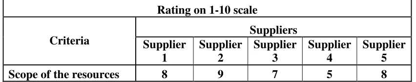
[image:43.612.104.530.633.717.2]For example, consider an ad-hoc method in which the criteria are measured in terms of a 1-10 scale with “10” being the highest score for a particular supplier and “1” being the lowest so as to be on the same terms or units as the other criteria (objectives) which will help optimize the objectives together.
Table 6.1
Rating on 1-10 scale
Suppliers Criteria Supplier
1
Supplier 2
Supplier 3
Supplier 4
Supplier 5
Reputation of the
supplier 9 10 6 6 9
Cultural barrier 10 10 10 8 6
Risk 10 9 9 7 8
Existing relationship 9 6 2 8 4 Additional value-added
capability 7 8 6 4 5
The decision maker will specify certain target values for each objective (criterion) to be achieved. For example, the decision maker will specify that all the suppliers scoring above “7” in the criteria “scope of the resources,” “reputation of the supplier,” and “cultural barrier” and above “5” in the criteria “risk,” “existing relationship,” and “additional value-added capability,” must be selected.
The automatic screening of the suppliers can be done based on the targets specified by the decision maker for the attributes, “scope of the resources,” “reputation of the supplier,” “cultural barrier,” “risk,” “existing relationship,” and “additional value-added capability,” the supplier list can be narrowed to a smaller set.
Based on the scores indicated in the table and the target values given by the decision maker, the qualified suppliers are “Supplier 1” and “Supplier 2.”
Similarly, one of the methods from MADM can be applied to arrive at the optimal decision for these criteria. This thesis study concentrates mainly on multi-objective decision making and not on multi-attribute decision making which is again a vast field of study. Hence, these criteria are not within the scope of the study in this thesis.
CHAPTER 7
7. MULTI-OBJECTIVE DECISION MAKING METHODS AND EXAMPLES
7.1 Introduction
Once the decision to outsource has been made by the company, the next most important activity or challenge to the company is the selection of suppliers. The right supplier will lead to the fulfillment of the company’s needs and a long-term relationship (Wadhwa and Ravindran 3726). It will help increase the financial stability as well as the reputation of the company in the market. Selection of the right supplier is a difficult task. It is possible that some suppliers may satisfy four criteria from a set of nine selected criteria but not satisfy the remaining five and some suppliers may satisfy the other five criteria but not the first four. Studies have shown that these criteria vary from product to product and also by the presence of quality programs within the business (Thaver and Wilcock 56). Thus, this highlights the fact that supplier selection problems are multi-objective problems and not single objective problems. Some criteria are quantitative whereas some are qualitative. No single methodology appears to be dominant in solving the supplier selection problem.
The need to resolve conflicting and multiple objectives in the current supply chain scenarios such as supplier selection requires additional research focusing on the multi-objective methods that will lead to suitable optimization models. For a company to stay competitive in the marketplace, it has to adopt different business strategies. Use of multi-objective optimization techniques to solve the multiple objectives of supply chain scenarios would lead to proper treatment of all critical objectives.
of solutions will be generated and presented to the decision maker in order to reach the final solution. A non-dominated solution is the one in which no objective function can be improved without degrading simultaneously at least one of the other objective functions. A solution can not be chosen as a better solution from a set of non-dominated solutions mathematically. The preference information from the decision maker (DM) is needed to reduce the set of non-dominated solutions as well as in arriving at the final solution. Hwang et al. presented the taxonomy of numerous multi-objective models that use the preference information given by the decision maker to the analyst at a particular stage (8):
1. No articulation of preference information
• • •
• No need for any information from the decision maker to the analyst once the
objectives and the constraints are set-up.
• • •
• Decision maker will accept solution obtained from the method. •
• •
• The advantage is the decision maker is not disturbed by the analyst which may
be preferred by the decision maker.
• • •
• The disadvantage is that analyst needs to make many assumptions about the
decision maker’s preferences which is difficult to do with even the best and knowledgeable analyst.
2. A priori articulation of preference information
• • •
• Preference information is given to the analyst by the decision maker before he
solves the problem.
• • •
• The information may be given in two ways, the decision maker will give some
judgment about specific objective preference levels or he will rank the objectives in order of their importance.
3. Progressive articulation of preference information (Interactive Methods)
• • •
• These methods are known as interactive methods. •
• •
• At each iteration of solution, preference information is expected from the
these cases but he gives the preference information on a local level to a particular solution(s) presented.
• • •
• After the limited number of interactions with the decision maker, these
methods lead him to the final/ preferred solution.
• • •
• The disadvantage is that the decision maker is asked to be involved frequently
as compared to other methods.
4. A Posteriori articulation of preference information (Non-dominated Solutions Generation Methods)
• • •
• In this method, the analyst presents the subset of the complete set of
non-dominated solutions to the decision maker and the decision maker then implicitly uses the trade-off information in order to select the preferred solution.
• • •
• The disadvantage is that there are too many solutions presented to the decision
Figure 7.1: Taxonomy of Multi-objective Decision Making Methods
Source: Hwang, C. L., S. R. Paidy, K. Yoon, and A. S. M. Masud. Multiobjective Decision Making – Methods and Applications. New York: Springer-Verlag Berlin
In this study various criteria would be considered and different multi-criteria methodologies would be studied against more prevalent criteria (supplier selection) and a heuristic methodology would be developed to find a suitable solution. An optimization model would be developed that is best suited for the procurement of the services from the suppliers which can be both local as well as overseas. This model further can also be applied to the procurement of the raw material from the suppliers. The development process will study and contrast various optimization methods being used in the previous research in a variety of problems and use an innovative methodology to solve the supplier selection problem. The methods include the weighted objective method, the goal programming method, the evolutionary algorithm method and the STEM method.
The different multi-objective methods used in this study to solve the supplier selection problem are:
1. Weighted Objective Method (Hwang et al. 32):
This priori articulation method scalarizes a set of objectives into a single objective by pre-multiplying each objective with the user-supplied weight. This method is one of the simplest to optimize a multi-objective problem. For example, if there are two objectives such as minimizing the cost and maximizing the production of a particular product in a company manufacturing two types of products, one would apply weights to these two objectives as indicated by the decision maker and optimize the problem easily. If the cost to be minimized is of high importance to the company as compared to the production of the specific product, the decision maker would give more weight to the cost variable than the product variable.
2. Goal Programming Method (Hwang et al. 56):
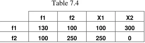
achieved are articulated by the decision maker. For example, suppose in a doll manufacturing company, the company manufactures two types of dolls ‘A’ and ‘B’. For each doll ‘A’ sold, the company makes $ 0.4 profit and for each doll ‘B’ sold, the company makes $ 0.3 profit. Doll ‘A’ requires twice the time to manufacture as compared to that of doll ‘B’. Two objectives the company has are to maximize the profit and maximize the production of product ‘A’. The raw material available for each day’s production of dolls ‘A’ and ‘B’ is limited to only 400. After calculation, the company finds out that the maximum number of doll ‘A’ it can produce is 250 and 0 of doll ‘B’, whereas if one customer asks for 300 dolls of type ‘A’, it falls short of the raw material. In such a situation, the decision maker must specify the priority of his goals. He may specify his first goal, to avoid the over usage of the raw materials, second to satisfy the closest customer by producing as many number of product ‘A’ as possible and the last priority is to maximize the profit as much as possible.
3. Evolutionary Algorithm Method:
There are many different types of evolutionary algorithms such as genetic algorithms, evolutionary strategies, genetic programming and evolutionary programming (Pinto). The basic working principle/logic of genetic algorithm is as explained below (Pinto):
• • •
• Create random population of ‘n’ individuals. •
• •
• These solutions are then compared and evaluated against the fitness
function.
• • •
• Create new members for the next population using the reproductive
operators: crossover and mutation.
• • •
• If the non-dominated set falls below the pre-specified level then there is no
need for increase in population size.
4. STEM Method (Hwang et al. 170):
The STEM method falls under the “Progressive articulation of Preference Information” category. The trade-off information is implicitly specified to the analyst by the decision maker. Trade-off information is the ratio of change in one objective function to the change in another objective function. In the STEM method, multiple phases of computation and decision making are interactive. Hence it allows the decision maker to recognize good solutions and the relative importance of the objectives. A pay-off table (usually a set of solutions in which one of the objectives is at its optimum) is constructed before the first interactive cycle and the best solution is found from it using a min-max strategy where the objective is to minimize the maximum deviation of an objective from its optimal solution. This step is analogous to the Global Criterion method where no articulation of preference information is needed. The cycle keeps repeating, at the mth cycle, the feasible solution is presented to the decision maker, which is the closest solution to the optimal value. The decision maker then compares this value to the ideal solution, if more iterations are required, the decision maker needs to relax some satisfactory objectives in order to improve unsatisfactory ones. The process cycle continues until the decision maker is satisfied with the solution.
7.2 Weighted Objective Method
Weighing objectives to obtain an efficient or pareto-optimal solution is one of the oldest multi-objective solution techniques (Wadhwa and Ravindran 3730). This method scales a set of objectives into a single objective by pre-multiplying each objective with the user supplied weight. It is the simplest way to apply if there are a number of objectives to be optimized. Weighted means are used by the statisticians to compensate for the presence of bias. It is used to give some elements or objectives more weight than others.
It has been shown that line passing through the point of tangency of indifference curve and non-dominated solution set is a source of the optimal values for the weight (Hwang et al. 32), i.e. slope of the tangent is proportional to the ratio of the optimal values of the weights. Thus if the optimal weights can be determined, the multi-objective problem will ensure the most satisfactory solution. However, in practice the weights often are the decision maker’s subjective estimate of the importance of different objectives and not necessarily the optimal values (Hwang et al. 32).
Similar to the two sided coin concept, this method also has its own advantages as well as disadvantages. The advantage of this method is that it is easier to get the weights from the decision maker, who may believe these values are correctly known before the actual solution. The disadvantage of this approach is that the weights depend on the achievement level of the objective functions and relative achievement of the objective functions compared to the achievement levels of the other objective functions (Hwang et al. 32).
decision maker would give more weight to the cost function rather than the product function.
Maximize: w1F1 + w2F2
Subject to: gi (x) ≤ 0 V i = 1, 2, 3……….n
where w1, w2 are the weights on each of the objectives F1 and F2 respectively. The
optimal solution to the weighted problem is a non-inferior solution to the multi-objective problem as long as all the weights are positive. The weights can be systematically varied to generate several efficient solutions. The weighting method is generally used to approximate the efficient set; it is not a good method for finding an exact representation of the efficient solution.
Example:
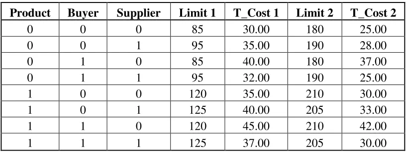
The following example by Wadhwa, Ravindran is illustrated and used in the paper “Supplier Selection in Outsourcing.” This is a supply chain problem in which buyers have to select the suppliers based on the various criteria that buyers decide upon. Often in the supplier selection problem, buyers have a dilemma due to the volume discounts offered by the suppliers, which depend on the volume of the order placed. The criteria considered in this problem for the selection of the potential suppliers are:
Price: Total cost of the purchasing of the parts from the suppliers consists of two factors, Fixed Cost and Variable Cost.
Lead Time: Lead time is the summation of the product of lead time for each part and the quantity of the parts being ordered. Lead time is measured in terms of days.
the parts received by the quality department of the company. It is measured in terms of percent of rejections.
The principal set of indices used to denote the various entities such as customers, parts, suppliers, etc. are shown in Table 7.1:
Table 7.1
INDEX ENTITY QUANTITY
i Part 2
j Buyer 2
k Supplier 2
m
Incremental Price
Break 2
Parameters used in the problem are:
• • •
• Pikm: Cost of acquiring unit of part i from supplier k at price level m,
V i, k, m = 0, 1
• • •
• Fk: Fixed Cost associated with each supplier, V k = 0, 1
F1 = 3500
F2 = 3600 •
• •
• dij: Demand of part i by buyer j, V i & j = 0, 1
d00 = 150
d01 = 175
d10 = 200
d11 = 180 •
• •
• qik: Quality that supplier maintains for part i,
q00 = 0.03
q01 = 0.09
q10 = 0.06
q11 = 0.02
• • •
• lijk: Lead time of supplier k to produce and supply part i to buyer j,
l010 = 17
l001 = 19
l011 = 18
l100 = 24
l110 = 21
l101 = 11
l111 = 12 •
• •
• CAPk: Production capacity of supplier k for part i,
CAP0 = 300 V i = 0
CAP0 = 350 V i = 1
CAP1 = 280 V i = 0
CAP1 = 360 V i = 1 •
• •
• bikm: Quantity at which price break occurs for part i given by supplier k for
buyer j,
b000 = 85 V j = 0, 1
b010 = 95 V j = 0, 1
b001 = 180 V j = 0, 1
b011 = 190 V j = 0, 1
b100 = 120 V j = 0, 1
b110 = 125 V j = 0, 1
b101 = 210 V j = 0, 1
b111 = 205 V j = 0, 1 •
• •
• Lij: Lead time that buyer j requires for part i,
L00 = 18
L01 = 20
L10 = 26
L11 = 13 •
• •
• Qj: Quality level that buyer j requires all suppliers to maintain,
Q0 = 0.095
Q1 = 0.09
Decision variables used in the model are:
• • •
• Xijkm: Number of units of part i supplied by supplier k to buyer j at price
level m
• • •
• Zk: It is a binary variable which denotes whether a supplier is selected or
not
• • •
• Yijkm: Also a binary variable which denotes which price level is selected
The problem consists of three objectives: 1. To minimize the total purchasing cost:
Total Variable Cost: ∑
i∑j∑k∑mPikm
. X
ijkm
Fixed Cost: ∑
k Fk . Zk
Hence, MIN ∑
i∑j∑k∑mPikm
. X
ijkm + ∑
k Fk . Zk
2. To minimize the lead time: MIN ∑
i∑j∑k∑m lijk
. X
ijkm
3. To minimize the number of part rejections: MIN ∑
i∑j∑k∑m qik
. X
ijkm
Under the weighted objective method, the above problem is transformed into the following single objective optimization problem:
MIN w1 ( ∑
i∑j∑k∑mPikm
. X
ijkm + ∑
k Fk . Zk ) + w2 ( ∑i∑j∑k∑m lijk
. X
ijkm ) +
w3 ( ∑
i∑j∑k∑m qik
. X
ijkm )
where w1, w2 and w3 are weights
The problem has the following constraints:
∑
i∑j∑mXijkm≤ (CAPk ) Zk V k = 0, 1
2. Demand Constraint: The demand of buyer j for part i has to be satisfied.
∑
k∑mXijkm = dij V i,j
3. Maximum number of selected suppliers: Maximum number of selected suppliers should be less than the number of participating suppliers
∑
k Zk≤ N
4. Linearizing constraints:
Solution:
The solution according to the paper “Supplier Selection in Outsourcing” by Wadhwa and Ravindran (2007) is as follows,
7.3 Goal Programming Method
Goals are the objectives or targets desired by the decision maker expressed in terms of a specific state in space and time. Thus, while objectives give the desired direction, goals give a desired target level to achieve.
Goal Programming was originally proposed by Charnes and Cooper for a linear model, which was further developed by Ijiri, Lee and Ignizio (Hwang et al. 56). The method requires the decision maker, to set the goals (targets) for the multiple objectives that are ranked according to the priorities in which they need to be achieved. The importance of these goals and the order in which they need to be achieved are articulated by the decision maker. A preferred solution is thus defined as the one which minimizes the deviations from the set goals. Given a portfolio of properly established goals, one tries to achieve them as closely as possible (Wadhwa and Ravindran 3731).
Goal programming is a three step approach as follows (Wadhwa and Ravindran 3731):
Step 1: Get the goals (targets) from the decision maker to be achieved for each objective. Goals are not constraints. Hence some may not be achievable.
For example, for objective function Fi whose target value is Bi; the
goal constraint is written as,
Fi (x) + di
- di +
= Bi
Where, di
= underachievement of goal di
+
Step 2: Get decision maker’s preference on achieving the goals. The preference information can be provided in one of three possible ways:
a. Ordinal: Objectives are ranked according to preference of order by the decision maker.
b. Cardinal: Specific weights are specified by the decision maker for each objective according to the preference order. c. Hybrid: This consists of ranking and weights both being specified
by the decision maker.
Step 3: Find an optimal solution that will be as close as possible to the stated goals, in the specified preference order.
The goal programming problem may be the linear integer goal programming problem or the non-linear integer goal programming problem. The deviations are to be minimized as much as possible. A lower ranking achievement function cannot be satisfied for the detriment function (Hwang et al. 57). The same problem can be solved using the iterative goal programming method. Using the method of linear approximation of non-linear functions, the non-linear goal programming problem can be solved by linear goal programming (Hwang et al. 57).
In this thesis the iterative goal programming method approach is used. The goal programming advantage is that the decision maker can give rankings instead of specifying weights to each objective function. The goal programming method has been widely used in many multi-objective decision making problems (Hwang et al. 58).
company has are to maximize the profit and maximize the production of product ‘A’. The raw material available for each day’s production of dolls ‘A’ and ‘B’ is limited to only 400. After calculation, the company finds out that the maximum number of doll ‘A’ it can produce is 250 and 0 of doll ‘B’, whereas if one customer asks for 300 dolls of type ‘A’, it falls short of the raw material. In such a situation, the decision maker must specify the priority of his goals. He may specify his first goal, to avoid the over usage of the raw materials, second to satisfy the closest customer by producing as many number of product ‘A’ as possible and the last priority is to maximize the profit as much as possible.
Example:
The following example is illustrated and used in the paper “Vendor Selection in Outsourcing” by Wadhwa and Ravindran. This is a supply chain problem in which buyers have to select the suppliers based on the various criteria that buyers decide upon. Often in the supplier selection problem, buyers are in the dilemma due to the volume discounts offered by the suppliers, which depend on the volume of the order placed. The criteria considered in this problem for the selection of the potential suppliers are:
Price: Total cost of the purchasing of the parts from the suppliers consists of two factors, Fixed Cost and Variable Cost.
Lead Time: Lead time is the summation of the product of lead time for each part and the quantity of the parts being ordered. Lead time is measured in terms of days.
Step 1: The decision maker has specified some goals for the three objectives. The problem is solved in the ideal condition and the ideal solution for the three objectives, namely, minimizing price, lead time and quality is found. The target values or the goals are set to 90% of their ideal values. The target values for price, lead time and quality are 102933, 12867 and 21.8 respectively.
Step 2: The order in which the objectives are prioritized is shown below: a. Minimum Cost
b. Minimum Lead Time
c. Minimum Percent of Rejections
Step 3: Analysis:
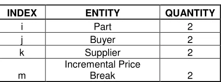
The principal set of indices used to denote the various entities such as customers, parts, suppliers, etc. are shown in Table 7.2:
Table 7.2
INDEX ENTITY QUANTITY
i Part 2
j Buyer 2
k Supplier 2
m
Incremental Price
Break 2
Parameters used in the problem are:
• • •
• Pikm: Cost of acquiring unit of part i from supplier k at price level m,
V i, k, m = 0, 1
• • •
• Fk: Fixed Cost associated with each supplier, V k = 0, 1
F1 = 3500
F2 = 3600 •
• •
• dij: Demand of part i by buyer j, V i & j = 0, 1
d01 = 175
d10 = 200
d11 = 180 •
• •
• qik: Quality that supplier maintains for part i,
q00 = 0.03
q01 = 0.09
q10 = 0.06
q11 = 0.02 •
• •
• lijk: Lead time of supplier k to produce and supply part i to buyer j,
l000 = 15
l010 = 17
l001 = 19
l011 = 18
l100 = 24
l110 = 21
l101 = 11
l111 = 12 •
• •
• CAPk: Production capacity of supplier k for part i,
CAP0 = 300 V i = 0
CAP0 = 350 V i = 1
CAP1 = 280 V i = 0
CAP1 = 360 V i = 1 •
• •
• bikm: Quantity at which price break occurs for part i given by supplier k for
buyer j,
b000 = 85 V j = 0, 1
b010 = 95 V j = 0, 1
b001 = 180 V j = 0, 1
b011 = 190 V j = 0, 1
b100 = 120 V j = 0, 1
b110 = 125 V j = 0, 1
b111 = 205 V j = 0, 1 •
• •
• Lij: Lead time that buyer j requires for part i,
L00 = 18
L01 = 20
L10 = 26
L11 = 13 •
• •
• Qj: Quality level that buyer j requires all suppliers to maintain,
Q0 = 0.095
Q1 = 0.09 •
• •
• N: Maximum number of suppliers that can be selected
Decision variables used in the model are:
• • •
• Xijkm: Number of units of part i supplied by supplier k to buyer j at price
level m
• • •
• Zk: It is a binary variable which denotes whether a supplier is selected or
not
• • •
• Yijkm: Also a binary variable which denotes which price level is selected
The problem consists of three objectives:
1. To minimize the total purchasing cost: Total Variable Cost: ∑
i∑j∑k∑mPikm
. X
ijkm
Fixed Cost: ∑
k Fk . Zk
Hence, MIN ∑
i∑j∑k∑mPikm
. X
ijkm + ∑
k Fk . Zk
2. To minimize the lead time: MIN ∑
i∑j∑k∑m lijk
. X
3. To minimize the number of part rejections: MIN ∑
i∑j∑k∑m qik
. X
ijkm
The problem has the following constraints:
1. Capacity Constraint: Each supplier k has maximum capacity CAPk,
∑
i∑j∑mXijkm≤ (CAPk ) Zk V k = 0, 1
2. Demand Constraint: The demand of buyer j for part i has to be satisfied.
∑
k∑mXijkm = dij V i,j
3. Maximum number of selected suppliers: Maximum number of selected suppliers should be less than the number of participating suppliers
∑
k Zk≤ N
4. Linearizing constraints:
Iteration 1:
MIN d1 +
SUBJECT TO
∑
i∑j∑mXijkm≤ (CAPk ) Zk
∑
k∑mXijkm = dij
∑
k Zk≤ N
∑
i∑j∑k∑mPikm
. X
ijkm + ∑
k Fk . Zk + d1
- d1 +
Iteration 2:
MIN d2 +
SUBJECT TO
∑
i∑j∑k∑mPikm
. X
ijkm + ∑
k Fk . Zk≤ 102933
∑
i∑j∑mXijkm≤ (CAPk ) Zk
∑
k∑mXijkm = dij
∑
k Zk≤ N
∑
i∑j∑k∑m lijk
. X
ijkm + d2
- d2 +
= 12867
Iteration 3:
MIN d3 +
SUBJECT TO
∑
i∑j∑k∑mPikm
. X
ijkm + ∑
k Fk . Zk≤ 102933
∑
i∑j∑k∑m lijk
. X
ijkm≤ 12867
∑
i∑j∑mXijkm≤ (CAPk ) Zk
∑
k∑mXijkm = dij
∑
k Zk≤ N
∑
i∑j∑k∑m qik
. X
ijkm + d3
- d3 +
= 21.8
Solution:
The solution according to the paper “Supplier Selection in Outsourcing” by Wadhwa and Ravindran (2007) is as follows,
7.4 Evolutionary Algorithm Method
Evolutionary algorithms are optimization algorithms that use the Darwinian theory of natural selection as the basis for optimization (Pinto). Evolution, which is a result of natural selection, is an optimization method which has had the luxury of having many years to complete its optimization or at least reach some kind of stable equilibrium. Evolutionary algorithms mimicking this behavior were first thought of for use in optimization by Prof. John H. Holland of the University of Michigan at Ann Arbor (Pinto).
The evolutionary algorithm mimics nature’s evolutionary principles to drive its search toward an optimal solution. Since a number of individuals are processed for each generation, the outcome of an evolutionary algorithm is also a population of solutions. If the optimization problem has a single optimum, all evolutionary algorithm population individuals can be expected to converge to that optimum. This ability to find multiple optimal solutions in one single simulation run makes evolutionary algorithms suitable in solving multi-objective optimization problems. Evolutionary algorithms are reported to give robust results (Pinto).
A considerable number of evolutionary algorithms have been proposed in the last few years (Belgasmi et al. 11). Some of them are genetic algorithms, evolutionary strategies, genetic programming and evolutionary programming (Pinto). Genetic algorithms are iterative and require a certain number of iterations to converge to the optimal solution. The basic working principle/logic of a genetic algorithm is explained below (Pinto):
a. Create random population of ‘n’ individuals.
b. These solutions are then compared and evaluated against the fitness function.
d. If the non-dominated set falls below the pre-specified level then there is no need for increase in population size.
Crossover combines two or more individuals to create a new individual while mutation is performed on a single parent by mutating one or more parameters. Crossover and mutation are the diversity operators that bring diversity to the present population. Research in multi-objective genetic algorithms came about with the development of the Vector Evaluated Genetic Algorithm (VEGA) and the Multi-Objective Genetic Algorithm (MOGA). Later on the Non-dominated Sorting Genetic Algorithm (NSGA) was presented by Srinivas and Deb in 1994 and in 2002 NSGA-II was being developed by Deb et al.
Evolutionary algorithms are sometimes called genetic algorithms (Day). Basic steps described by Day are:
a. Each objective function is solved and its value is determined. b. Pairs of individuals are selected to reproduce.
c. Individuals are forced to undergo Crossover. d. Mutation is performed on the individuals.
e. Fitness test is performed on the children produced. f. Steps are repeated until the destination is reached.
Example:
The following example is illustrated and used in the paper “Supply Chain Optimization using Multi-Objective Evolutionary Algorithms” by Pinto.
Pinto has implemented the Non-dominated Sorting Genetic Algorithm-II in a three stage supply chain problem. The three stages are:
a. Supplier b. Plant
The decision maker has various objectives to be achieved such as minimizing the total operating cost, manufacturing cost, transportation cost and maximizing the profit, revenue. The problem is formulated in such a way that two objective functions are clubbed together in each set to form 4 sets in total and constraints are selected depending on the set of objective functions used.
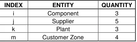
[image:69.612.203.431.279.350.2]Principal set of indices used to denote the various entities such as components, suppliers, plants, etc. are as shown in Table 7.3:
Table 7.3
INDEX ENTITY QUANTITY
i Component 3
j Supplier 5
k Plant 3
m Customer Zone 4
Parameters used in the problem are:
• • •
• Lij: Capacity of supplier j for component i •
• •
• CSij: Cost of making a component i by supplier j •
• •
• STCijk: Transportation Cost of component i from supplier j to plant k / unit •
• •
• Uk: Capacity of plant k •
• •
• LCk: Labor Cost of plant k / unit •
• •
• MCk: Manufacturing Cost of plant k / unit •
• •
• ICk: Inventory Cost of plant k / unit •
• •
• PTCkl: Plant Transportation Cost from plant k to customer zone l / unit •
• •
• Dl: Demand at customer zone l •
• •
• SPl: Selling price at customer zone l / unit •
• •
• Sij: Binary variable denoting whether component i can be supplied by
supplier j or not.
Decision variables used in the model are:
• • •
• Xijk: Number of components i from supplier j to plant k •
• •
• • •
• Iik: Inventory of component i at plant k
Objective Functions:
Set 1: MIN Total Operating Cost (TOC)
MIN Manufacturing Cost (MC) / Total Operating Cost (TOC)
Set 2: MAX Profit
MIN Manufacturing Cost (MC)
Set 3: MAX Revenue
MIN Manufacturing Cost (MC)
Set 4: MAX Revenue
MIN Transportation Cost (TC)
TC = ∑
i∑j∑k Xijk
. S
ij . STCijk + ∑
k∑l Ykl
. PTC
kl
Total MC (TMC) = ∑
k LCk + MCk + ICk
Supplier Cost (SC) = ∑
i∑j CSij
. S
ij. Xijk
TOC = TC + TMC + SC
Constraints:
1. Capacity Constraint:
a. Plant Capacity: ∑
l Ykl ≤ Uk V k = 0, 1, 2
b. Supplier Capacity: ∑
k Sij
. X