Rochester Institute of Technology
RIT Scholar Works
Theses
Thesis/Dissertation Collections
5-30-2008
A Comparative Study of the Robustness of Voting
Systems Under Various Models of Noise
Derek M. Shockey
Follow this and additional works at:
http://scholarworks.rit.edu/theses
Recommended Citation
A Comparative Study of the Robustness of Voting
Systems Under Various Models of Noise
Derek M. Shockey 30 May 2008
Chair: Christopher M. Homan
Reader: Piotr Faliszewski
1453880
1453880
Contents
1 Introduction 1
2 Background 6
2.1 History of Social Choice . . . 6
2.2 Notation . . . 10
2.3 Definitions of Voting Rules . . . 11
2.3.1 Scoring Rules . . . 11
2.3.2 Copeland [11, 27] . . . 12
2.3.3 Maximin [25, 30] . . . 12
2.3.4 Bucklin [7] . . . 12
2.3.5 Plurality with Runoff [9] . . . 13
3 Robustness in Voting 14 3.1 Overview . . . 15
3.3 Theorems . . . 17
3.4 Scoring Rules . . . 20
3.5 Copeland . . . 21
3.6 Maximin . . . 23
3.7 Bucklin . . . 24
3.8 Plurality with Runoff . . . 25
4 Experimental Bounds on Robustness 30 4.1 Overview . . . 30
4.2 Results for Arbitrary Reordering . . . 33
4.3 Results for Elementary Transposition . . . 34
5 Conclusion 35 A Suppression 38 A.1 Definitions . . . 38
A.2 Theorems . . . 39
B Source Code 41
Abstract
While the study of election theory is not a new field in and of itself, recent research has applied various concepts in computer science to the study of social choice theory, which includes election theory. From a security per-spective, it is pertinent to investigate how stable election systems are in the face of noise, disruption, and manipulation. Recently, work related to com-putational election systems has also been of interest to artificial intelligence researchers, where it is incorporated into the decision-making processes of distributed systems. The quantitative analysis of a voting rule’s resistance to noise is therobustness, the probability of how likely the outcome of the election is to change given a certain amount of noise. Prior research has studied the robustness of voting rules under very small amounts of noise, e.g. swapping the ranking of two adjacent candidates in one vote. Our re-search expands upon this previous work by considering a more disruptive form of noise: an arbitrary reordering of an entire vote. Given k noise
disruptions, we determine how likely the election is to remain unchanged (the k-robustness) by relating the k-robustness to the 1-robustness. We
Acknowledgements
Chapter 1
Introduction
Multiple-winner elections are also common for electing officials to multiple-member legislative bodies, usually by proportionally distributing seats based on the number of votes for each party (rather than votes for a specific candi-date). This system is used for the lower house of parliament in France (the French National Assembly) and both houses of parliament in Italy. The lower house of the German parliament (the Bundestag) is elected half by a proportional multiple-winner election, and half by single-winner plurality elections. There are also non-proportional multiple-winner voting systems, which usually fill the n positions with the top n plurality winners, called
bloc voting or plurality-at-large. Generally, a bloc voting system is used for smaller governing bodies, such as a council or a board, though there are instances of legislative bodies being elected by non-proportional voting systems.
The above examples of political elections are founded on a basic principle of “one person, one vote,” giving each citizen an equal say. Outside of the world of politics, this is rarely the case. In corporate elections, for example, each shareholder may vote on issues such as who serves on the board of directors, approval of sales and acquisitions, etc., but the votes of a shareholder are weighted by the number of shares owned. This allows any person or entity owning a majority of shares to retain control of the company, as the majority shareholder cannot be outvoted. Furthermore, corporations can issue different classes of shares with different voting rights. This could allow for a non-majority shareholder to still retain the majority of voting rights, and therefore retain control of the corporation.
Since the 13th century, mathematicians have studied methods for conducting elections, which allow a group of voters to express their opinions on a given set of candidates or issues. It would be reasonable to say that the outcome of an election must best represent the aggregate preferences of the voters, or the election has essentially failed its purpose. The study of elections and voting rules has evolved into the field of preference aggregation, a major component of social choice theory.
account. Resulting from extensive study of social choice mechanisms, many alternative election systems have been developed based on entirely different and more complex mathematical functions that weight the rankings of all the candidates; we will explore several of these, including Copeland, Bucklin, and Maximin.
Most likely, the complexities of these election systems have prevented their widespread use in political elections, even though they may yield a winner who, in some respects, more accurately represents the preferences of the voters. The concerns of practicality are greatly mitigated in an electronic context, however, and as a result the study of preference aggregation has become increasingly relevant in multiagent scenarios and important to the field of distributed artificial intelligence.
Conducting preference aggregation in an electronic context, especially when networked, obviously presents a variety of security issues, many of which have arisen during the deployment of electronic voting machines for use in political elections. The alteration of the aggregate data, whether intentional and malicious or accidental, clearly has the potential for enormous impact on modern society. While the threat pertaining to decision making in artificial intelligence may not seem as serious as in political elections, in both cases there are opportunities to compromise an entire system that utilizes these decision-making mechanisms.
One good measure to determine if a voting rule could be implemented prac-tically in these contexts is robustness. The measure of robustness is the quantitative analysis of the probability that the outcome of an election will not change when the election data is altered by a given amount of noise. The noise could in practice be either intentional manipulation of the data, or unintentional random corruption. The measure of robustness is in some ways applicable to both types, but the resistance of voting protocols to ma-nipulation is an entire topic in and of itself [4, 6, 10, 13, 16, 29] that is far beyond the scope of our research. We will instead focus our efforts on the notion of robustness in the face of random noise.
type of noise would ostensibly be random and unintentional. Procaccia et al. defines the term 1-robustness as being the probability the the outcome of an election remains unchanged after a single fault (one randomly chosen elementary transposition), andk-robustness as the probability of robustness
given multiple (k) faults. Comprising the bulk of the research in Procaccia
et al. are the upper and/or lower bounds in terms of k-robustness for five
different well-established election rules: scoring rules, Copeland, Maximin, Bucklin, and plurality with runoff. The bounds are all strictly worst case, although we discovered in our own work that it is very difficult to prove what specific distributions are actually the worst for a given election rule. Our intention is to expand upon this research using more severe types of noise and to study their effect on the outcomes of the same five election rules. Procaccia et al. equates a single transposition to the flip of a single bit in the bitwise encoding that they devised to represent ordinal preferences in an election. The representation is a rather contrived construct designed to provide a simple plausible explanation for even trivial amounts of noise to have a real impact on the election outcome. Rather than delve into the semantics of representation, we will waive this and suffice it to say that some noise simply results in a specific type of alteration which is more significant than a single transposition. As with Procaccia et al., the forms of noise are intended to be unintentional and uncontrolled corruption, but some of the expanded noise may also have applicability to malicious manipulation of the system.
with increased noise.
Chapter 2
Background
2.1
History of Social Choice
Most historians point to Athens, the ancient Greek city-state of circa 500
bce, as the birthplace of modern democracy. Though it is not generally
considered to be the first democratic state, it is noted to be the most stable and important of the ancient world. Its form of government became a model not only for other Greek cities, but remains an important model today. The word democracy itself is in fact Greek, meaning power or rule (kratos) by the people (demos). The fundamental principle of Athenian democracy was that it wasaggregative, providing the citizens an opportunity to influence the laws by which they are bound; this was in sharp contrast to the monarchies and oligarchies that preceded it. This basic tenet remains the foundation of modern democracies.
made famous by Jean-Charles de Borda in 1770, which we study in depth in this paper; another is the Condorcet criterion [26], described by the Marquis de Condorcet in 1785, which requires the winner of an election to be pre-ferred over every other candidate. We do not study the Condorcet criterion specifically, but two of the voting systems we do study, Copeland [11] and Maximin [25, 30], are Condorcet-compliant.
After the rediscovery of election theory by Condorcet and Borda in the late 1700s, new work continued through the next century, most notably by Charles Dodgson and Thomas Hare. Dodgson, more commonly known by his pen name Lewis Carroll as the author of Alice’s Adventures in Won-derland, was also a mathematician and election theorist. Proposed in an 1876 pamphlet, the system now known as Dodgson’s method is based upon the Condorcet criterion [26]. If there is no Condorcet winner, Dodgson pro-posed a method of determining a winner by choosing the candidate that is “closest” to meeting the criterion [26, 28].
Thomas Hare was a British lawyer and major proponent of electoral reform. Hare published several editions of his electoral theory work between 1857 and 1873, in which he created the Single Transferable Vote (STV) system still used in the Republic of Ireland and Australia [6], as well as the epony-mous Hare quota that is sometimes used with STV. Hare, along with fellow election reform proponent and Member of Parliament John Stuart Mill, also popularized the idea of proportional representation, which is now used in parliamentary elections of many European countries (though ironically not in his home country).
Though many of the foundations of voting theory were laid in the works of Llull, Borda, and Condorcet, the bulk of work has been conducted in the 20th century and beyond. Several of the voting systems we will study were conceived within the last century, including Copeland (1951) [11], Max-imin, also known as Simpson–Kramer [25,30] (1969, 1977) or Minimax, and Bucklin [7] (1911). Other widely-known modern election systems include Black [5], Coombs [8] and Kemeny–Young [23, 24, 31].
how social values can be imposed by a “set of individual orderings,” es-sentially a preference profile consisting of ranked votes, aggregated under a “constitution,” which is a voting rule that maps a set of orderings to one “social ordering.”
An important component of Arrow’s book is a theorem now commonly known as Arrow’s impossibility theorem, or Arrow’s paradox. Arrow de-creed four “reasonable” requirements of any voting system—unanimity (also called Pareto efficiency), unrestricted domain (also called universality), non-dictatorship, and independence of irrelevant alternatives—and mathemat-ically proves that no voting system allowing more than two choices can ever uphold all of these principles simultaneously. The theorem is some-times (controversially) condensed to statements such as “No voting method is fair.” These principles as written by Arrow quickly became an important framework for studying social choice that is still in place today.
In the past two decades, a new discipline has arisen known as computa-tional social choice, in which the studies and principles of computer science are applied to problems of social choice theory. The seminal work in this area is generally considered to be a 1989 article by Bartholdi, Tovey, and Trick [3]. This work provides a proof that in a Dodgson election, in terms of computational complexity it is NP-hard to simply determine if a particular candidate is a winner of the election. Perhaps more importantly, the work also provides a class of “impracticality theorems” which are somewhat anal-ogous to Arrow’s impossibility theorem, as they assert that any fair voting scheme must require excessive computation to determine a winner in the worst case.
Just a few months after their first article, Bartholdi, Tovey, and Trick pub-lished a second article [2] that specifically addresses computational complex-ity of manipulating an election, as well as an election system that is resistant to computational manipulation. This work provided much of the foundation for future study of computational complexity. Hemaspaandra, Hemaspaan-dra, and Rothe have written extensively on this subject in the past decade, covering topics such as the complexity of Dodgson elections [19], manipulat-ing elections to prevent a specific candidate from winnmanipulat-ing [21], and resistmanipulat-ing manipulation by using hybrid elections [20].
such a way that there are relatively few candidates, the work is able to provide specific bounds on the computational complexity of manipulating several different election rules. Both individual manipulation and “coali-tional” manipulation by several agents in concert were considered. Conitzer and Sandholm were able to determine that given information about other agents’ votes, manipulation is very easy, even by an individual agent, as long as votes are unweighted. They also concluded that manipulation under a system of weighted votes is generally intractable. The conclusions of this work and related works are generally that manipulation of an election is easy, especially if the intended manipulation is “destructive,” meaning the goal is simply to prevent one candidate from winning.
The emerging field of computational social choice was formalized in Decem-ber 2006 with its first international workshop [12]. It is from the proceedings of this conference that the primary basis for our research comes: a study on the robustness of election systems by Procaccia et al. [27]. The work is certainly not the first research pertaining to this field, however. Kalai [22] es-sentially studied robustness of elections, but without using the specific term “robustness.” Kalai’s work proposed the more general question of “How likely is it that small random mistakes in counting the votes in an election between two candidates will reverse the election’s outcome?” Assuming a uniform and independent distribution of preferences, the work uses social welfare functions with simple voting rules to analyze the robustness. Kalai also defined the notion of “social chaos,” which is related to the probability of finding cycles in the preferences. Interestingly, Kalai was also able to re-late the the robustness under random noise the likelihood that a candidate
ais preferred toc, given that ais preferred tob and bis preferred to c. As
a whole, Kalai’s work is concerned more with social welfare functions and random noise, rather than the specific voting rules and noise types of our research.
but rather to affect the outcome of the election in some way.
The robustness of an election is defined to be the probability for which an election’s outcome will remain unchanged given a certain disruption in the voting data. Procaccia et al. [27] investigates the robustness of vari-ous common voting systems with respect toelementary transpositions. An elementary transposition is essentially the least significant possible change that can be made to an election: in a single voter’s ranked preference list of candidates, the positions of two adjacent candidates are swapped. The work focuses specifically on the “1-robustness,” which is the probability of robustness given a single such transposition. Procaccia et al. provides up-per and/or lower bounds on the 1-robustness of five voting systems: scoring rules, Copeland, Maximin, Bucklin, and Plurality with Runoff.
2.2
Notation
Procaccia et al. [27] uses conventional social choice notation from Brams and Fishburn [6] to mathematically represent elections and their components. In order to assist in both viewing this work as an extension of Procaccia et al., as well as within the context of computational social choice, we will follow this same basic notation, with a few of our own additions.
Let the set of voters be V = {v1, v2, . . . , vn} and the set of candidates be
C={c1, c2, . . . , cm}wheren=|V|andm=|C|. The indexiin superscript
refers to voters, and the index j in subscript refers to candidates. The set
of all linear orders onC is denoted by L =L(C). Each voter ihas ordinal
preferences!i∈ Lwhere the candidates are rankedc
j1 !i cj2 !i · · ·!i cjm. !V=#!1, . . . ,!n$ ∈LN is apreference profile. πl(!i) denotes the candidate
that voter i ranks in the l’th position; similarly, the notation li
j indicates
the ranking of candidatecj in ordinal preference list !i. The winner of an
election is decided by the voting rule, which is a functionF :LV →C. This
2.3
Definitions of Voting Rules
The voting rules we have chosen to focus on are scoring rules, Copeland, Maximin, Bucklin, and plurality with runoff. It is intentional that these are the same rules studied in Procaccia et al. [27], as this allows us to make a direct comparison between the results on robustness of elementary transposition and arbitrary reordering. These rules are all firmly established and well-studied within the field of social choice. This section defines, both formally and informally, each of these rules. Though there is no one universal method for tie-breaking an election in which more than one candidate has the highest score, for the purposes of this work, a winning candidate will be selected arbitrarily from the set of candidates with the highest score.
2.3.1 Scoring Rules
Scoring rules are actually representative of a generic class of election rules, rather than a specific rule; however, since they can all be generically repre-sented in the same way, we can study them together. Scoring rules are based upon a scoring vector "α of size m that provides a score for each rank. A
candidate’s score in a given preference profile is simply the sum of its scores based on its rank in each vote. The formal definition is as follows: given a scoring vector "α =#α1, . . . ,αm$, the score of a candidate j is sj =!iαli
j,
and the winner of the election isF(!) = argmaxjsj.
Though the scoring vector"α is not constrained to any specific values, there
are some common scoring rules that have been studied (we were unable to find authoritative references for plurality and veto, but these definitions are widely accepted). Although our results are general and applicable to all scoring rule implementations, we will focus these specific scoring vectors for our experimental results:
• Borda: "α=#m−1, m−2, . . . ,0$[26] • Plurality: α" =#1,0, . . . ,0$
2.3.2 Copeland [11, 27]
The Copeland election rule is based upon the rankings of each candidate relative to every other candidate. A series of pairwise elections is conducted, each of which compares exactly two candidates to each other. The resulting scores of the pairwise election are simply the number of times each candidate was ranked higher than the other; the degree by which their ranks differ is not a factor. For Copeland, every candidate competes in a pairwise election against ever other candidate, and each candidate’s score is the number of other candidates they beat. In the original Copeland definition, ties were awarded half points; in some later works, including Procaccia et al. [27], this is not done. The formal definition of Copeland as used in Procaccia et al., and for the purposes of this work, is as follows:
Candidatejbeatsj! in a pairwise election if|{i:lij < lji!}|> n/2. The score
for candidate j, sj, is the number of candidates that j beats in pairwise
elections. The winner of the election Copeland(!) is argmaxjsj.
2.3.3 Maximin [25, 30]
Maximin, sometimes called Minimax or Simpson–Kramer, consists of a series of pairwise elections comparing each candidate to every other candidate, similar to Copeland. In Maximin, however, the candidate’s score is itsworst
pairwise score against the other candidates. The winner of the election is still the candidate with the highest score, however, which could be thought of as “the best of the worst.” Formally, the definition of Maximin is: The score of candidate j is sj = minj!|{i : lij < lji!}|, and the winner of
Maximin(!) is argmaxjsj.
2.3.4 Bucklin [7]
The Bucklin election system, while somewhat confusing in its mathematical definition, is fairly simple in principle. A candidate needs a majority score, more than half of n, to win. The election proceeds in rounds. The first
has a majority, the election proceeds to the second round, where the top two ranks are considered, and so forth, iterating through each successive rank. A candidate’s score is simply the total number of combined votes it has in all currently-considered ranks. If at any time a candidate reaches a majority score, the election is stopped, and that candidate is declared the winner. Formally, Bucklin is defined as:
For all candidatescj and l∈ {1, . . . , m}, let Bj,l ={i:lij ≤l}. The winner
of Bucklin(!) is argminj(min{l:|Bj,l|> n/2}).
2.3.5 Plurality with Runoff[9]
Plurality with Runoff is a hybrid election, which always consists of two rounds. The first round is a plurality election, as defined above in Scoring Rules; however, rather than a single winner, this first round returns the two candidates with the highest plurality scores. These two candidates proceed to a runoff election, which is pairwise. The runoff candidate with the higher pairwise score wins the overall election.
More formally, the two candidates who maximize|{i∈ N : lij = 1}|, move
Chapter 3
Robustness in Voting
Function TranspositionLower BoundReordering TranspositionUpper BoundReordering Scoring Rule m−1−aF
m−1
(# m
aF+1$!)aF+1
m!
m−aF
m 1−
2m(aF−1)−aF2−aF+1
2m!
Copeland 0∗ 0† 1
m−1 1−
(m+1)(m−1)!−2 2m!
Maximin 0∗ 0† 1
m−1 1−
(m−1)!−1
m!
Bucklin m−2
m−1
""m−1
2
#
!#2
m! 1∗ 1†
Plurality w. Runoff m−5/2
m−1 67m‡
m−5/2
m−1 + 5/2
[image:21.612.126.593.348.474.2]m(m−1) 9m4m−210‡
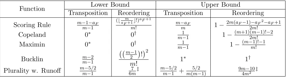
Table 3.1: Comparison of the upper and lower bounds of various scoring rules for elementary transposition and arbitrary reordering. The bounds for elementary transposition are from Procaccia et al. [27]; the bounds for arbitrary reordering are from our own work and discussed in detail in this chapter.
∗These bounds are as provided in [27], but it is unlikely they represent actual bounds.
In these cases the authors indicated they felt the actual bounds were inconsequential.
†These values are not intended to denote the actual bounds, but simply indicate these
particular values were beyond the scope of this work and have been replaced by the absolute minimum or maximum bound.
‡These bounds only hold for values of m ≥ 3, but we find this to be a reasonable
3.1
Overview
Recently, Procaccia et al. [27] conducted research on robustness in voting. Specifically, the work was focused on the the smallest possible amount of noise, the single elementary transposition. Procaccia et al. derived upper and/or lower bounds for five different established voting rules. The authors offer a specific binary representation of a preference profile in order to sup-plement their fault model. Specifically, the representation uses a single bit to represent each of the"m
2
#
candidate pairs; a value of 1 indicates the first candidate is preferred to the second, and a value of 0 is a preference for the second candidate over the first. While it is intuitive that this is not the most compact form of representation, which the authors note, they do elaborate on some advantages; specifically, there is the possibility to check for certain properties of the election in constant time using bitmasks. It has a major disadvantage in that it is possible to represent an inconsistent preference profile, in that there the transitivity can be violated. While this is not dif-ficult to detect, it is still an impossible occurrence in a more conventional list-based representation.
We will expand the notion of noise to include more significant alterations to the preference profile; specifically, we will examine the impact of a voter’s ordinal preferences being scrambled (arbitrarily reordered), which itself is actually equivalent to a series of elementary transpositions confined to the context of a single voter. In our preliminary research, we also investigated the notion of suppression, in which a single voter’s entire ordinal preference list is not considered in determining the election outcome; however, we were unable to obtain interesting results from this, and consequently removed it from the final work. The preliminary work regarding suppression can be found in Appendix A.
imple-mentation details to be generally irrelevant to the actual impact of the noise on the robustness of the election. Given these expanded criteria for noise, we will examine the effects on the k-robustness of the same election rules
as Procaccia et al. [27]: basic scoring rules (Plurality, Veto, and Borda), Copeland, Maximin, Bucklin, and Plurality with Runoff.
3.2
Definitions
Procaccia et al. [27] focuses exclusively on one type of noise, theelementary transposition. This consists of a swap between the rankings of two adjacent candidates in a single voter’s ordinal preference list, and is arguably the “smallest” amount of noise possible. As such, it can even be considered the building block of more exaggerated forms of noise, and we will use it as such. We include here the Procaccia et al. definition of elementary transposition:
Definition 1. A preference profile!V
1 is obtained from a preference profile
!V by anelementary transposition (write: !V!!V
1) if there exists a voter
vi and l∈ {2, . . . , m}such that:
1. for alli! (=i,!i!=!i1!
2. πl(!i) =c=πl−1(!i1)
3. πl−1(!i) =c! =πl(!i1)
4. !i↓
C\{c,c!}=!i1↓C\{c,c!}
The !i↓
C\{c,c!} notation is used by Procaccia et al. [27] without a specific
definition, but we understand it to be defined as the preference profile !i
with candidates{c, c!}removed from consideration.
Definition 2. Given a preference profile !V and a voter vi ∈V, the
pref-erence profile !V
1 is obtained from !V by anarbitrary reordering if for all
i! (=i,!i!=
!i!
1.
We measure the effects of noise on an election or voting rule in terms of robustness: the probability that given some sort of noise, disruption, or alteration of the preference profile data, the outcome of the election is un-affected. Specifically, we are interested in thek-robustness, which is defined
here as the probability of robustness givenkindependent noise faults: Definition 3. The k-robustness of a preference profile !V under an
arbi-trary reordering ofk voters vi ∈V for i= 1, . . . , k, written φk(!V) =!V1,
is:
ρφk(F,!
V) = Pr &V
1∼φk(&V) $
F(!V) =F(!V1)
% .
The notation!V
1∼ φk(!V) is adapted from Procaccia et al. [27], in which it
is defined to be the probability of obtaining!V
1 from!V bykfaults chosen
randomly and independently.
Once thek-robustness of the preference profile is established, it is
straight-forward to link the robustness to the voting rule itself:
Definition 4. Thek-robustness of a voting ruleF under arbitrary
reorder-ing of k voters vi ∈ V for i = 1, . . . , k with n voters and m candidates
is:
ρn,mφ
k (F) = min &V
1∈L(C)n
ρφk(F,!
V
1).
3.3
Theorems
Largely in order to simplify our contention that the arbitrary reordering is strongly linked to the elementary transposition, which consequently simpli-fies proofs of our work in relation to Procaccia et al. [27], we explicitly prove the relation:
Proposition 1. Every arbitrary reordering can be obtained by a series of at most m2−m
Proof. Since the arbitrary reordering is confined to a single voter’s ordinal preference list,!i, the elementary transpositions take place on one list of size
m, i.e.| !i|=m. It therefore can take at mostm−1 transpositions to get
the first list element in!i to match its position in the arbitrarily reordered
list; that is, to order the list such that π1(!i1) = π1(!i). Subsequently, it
will take at mostm−2 transpositions for the second element, m−3 for the
third, etc., resulting in the summation
m&−1
h=1
m−h. It is straightforward to
see that this summation is equal to m2−m
2 , which is the upper bound to obtain an arbitrary reordering via a series of elementary transpositions.
Following the proof of Proposition 1, it is a simple case to prove that an ar-bitrary reordering can alter the outcome of an election. Procaccia et al. [27] already proves this for elementary transpositions in Theorem 1, included below.
Theorem 1 [27]. LetF :LV →Cbe a voting rule such thatRange(F)>1.
Then there exists a preference profile!V and a profile !V
1 which is obtained
from!V by an elementary transposition, such thatF(!V)(=F(!V
1).
Theorem 2. Let F : LV → C be a voting rule such that Range(F) > 1.
Then there exists a preference profile!V and a profile !V
1 which is obtained
from!V by an arbitrary reordering, such thatF(!V)(=F(!V
1).
Proof. Since !V
1 can be obtained from !V by a series of elementary
trans-positions, per Proposition 1, the proof of this claim follows inherently from the Procaccia et al. [27] proof for Theorem 1.
To provide a link betweenk-robustness and 1-robustness, Procaccia et al. [27]
boundsk-robustness by thekth power of 1-robustness, as seen below in their
Proposition 2. We do the same, but define k in terms of an arbitrary
re-ordering.
Proposition 2 [27]. ρn,mk (F)≥(ρn,m1 (F))k.
Proposition 3. Givenk arbitrary reorderings, ρn,mφ
k (F)≥(ρ
n,m φ1 (F))
Proof. Consider the preference profile!V
1 and the preference profile!V
k
2
ob-tained from it bykindependent and random arbitrary reorderings. We claim
the probability thatF(!V
1) =F(!V
k
2 ) is at least (ρn,mφ1 )
k. Let!V
i1, . . . ,!
Vk
ik+1
be the intermediate preference profiles obtained by the reorderings, where
!V i1 =!
V
1, !V
k
ik+1 =!
V
2, and each !Vij+1 is obtained from !
V
ij by a random
and independent arbitrary reordering for j = 1, . . . , k. By the definition
of 1-robustness, for every preference profile !Vi
, the probability that one randomly chosen arbitrary reordering does not change the outcome of the election underF is at least ρn,mφ1 (F). Therefore, forj= 1, . . . , k,
Pr'F(!Vij) =F(!Vij+1) | !Vij(≥ρn,mφ (F).
Therefore:
Pr$F(!V1) =F(!V2)
%
=
k )
j=1
Pr'F(!Vij) =F(!
V
ij+1) | !
V ij (
≥ (ρn,mφ
1 )
k.
Above, we have used the concept of 1-robustness as a lower bound for thek
-robustness. This is done in the same manner as Procaccia et al. [27] and for exactly the same reasons: a high lower bound implies a high k-robustness,
while a low 1-robustness indicates that the k-robustness of the rule is not
worth considering.
Now that we have clearly defined our models for noise, as well as the def-initions of their robustness, we will apply these in order to examine the
k-robustness of the voting rules (Plurality, Veto, Borda, Copeland,
Max-imin, and Plurality with Runoff) in much the same manner as Procaccia et al. [27], with the exception of the definition of a fault. Rather than each of the k faults indicating a single elementary transposition, we will
rede-fine a fault within the context of our noise; that is,k instances of arbitrary
reordering.
we discuss, there arem candidates, and therefore in each vote there are m!
possible permutations, or arbitrary reorderings. We may refer to a set of permutations as “safe” if no permutation of that form can possibly alter the election outcome, thereby contributing to the quantification of robustness.
3.4
Scoring Rules
In this section, we attempt to quantify the robustness generally for all scoring rules. It is difficult to obtain meaningful results for such a broad class of rules, as the scoring vector "α significantly affects the resulting robustness.
Given a scoring rule F with scoring vector "α, let AF = {l ∈ {2, . . . , m} :
αl−1 > αl}, and aF = |AF|. The robustness of a scoring rule is strongly
linked to the parameter aF, as the scores can only change when the noise
violates the boundaries in the scoring vector. To find the lower bound for scoring rules, we claim that the worst case distribution is when each of the score groups contained within inAF are of equal size.
Proposition 1. Let n and m be the number of voters and candidates, and
let F be a scoring rule. Then ρn,m1 ≥ (, m aF+1-!)
aF+1
m! .
Proof. When there are aF divisions in the scoring vector, there are aF + 1
distinct groups of equal scores. One way to guarantee that the outcome of the election remains the same after a vote is reordered is to require that the reordering causes no candidate to “jump” across the divisions in AF that
bound each score group. For each of theaF + 1 groups of size rs, there are
rs! possible permutations that meet this restriction. Therefore, the total
number of acceptable permutations is
a)F+1
s=1
rs!.
This value must be minimized when the score groups in α" are as close to
equal as possible; that is, when the size of each group is between , m aF+1
-and. m
aF+1/. When this is the case, the probability that the outcome of the
electionF will not change must be at least (,
m aF+1-!)
aF+1
m! .
this case, we find that skewing the distribution to one end, just the opposite of the equal groupings used in the lower bound, allows us to provide a tighter upper bound.
Proposition 2. Let n and m be the number of voters and candidates, and
let F be a scoring rule. Then ρn,m1 ≤1−2m(aF −1)−aF
2−a
F + 1
2m! .
Proof. Given that there are aF + 1 groups of equal scores in the scoring
vector "α, we can guarantee a change in the outcome of the election F by
strictly increasing the score of one candidate while strictly decreasing the score of another. We can accomplish this by reordering a vote such that two candidates associated with different score groups switch places in the ordinal preferences, as long as neither of the candidates is the winning candidate
cW.
For each candidatecj ∈C, we can swap with any of the othermcandidates,
less the candidates in cj’s own scoring group and the winning candidate
cW. Denoting the size of candidate cj’s scoring group as ajF, the number of
such swaps is the sum &
j∈C−{cW}
m−ajF −1. Removing the constant terms
yields the sum (m−1)2− &
j∈C−{cW}
ajF. In order to maximize the number
of outcome-altering reorderings,aF of the score groups in "αmust be of size
1, and one such group must contain the winning candidate. The remaining score group is of size (m−aF). Since ajF = 1 for all but one score group,
the expanded summation is (m−1)2−aF −(m−aF)2. To correct double
counting, this entire value is divided by 2. Subtracting from 1 to find the robustness, the result is 1−2m(aF −1)−aF
2−a
F + 1
2m! .
3.5
Copeland
rank of the candidate within any randomly selected vote is irrelevant in considering the robustness of the rule.
Proposition 3. Let m be the number of candidates, and let n, the number
of voters, be even. Thenρn,m1 (Copeland)≤1−(m+ 1)(m−1)!−2
2m! .
Proof. Consider an election in which for i = 1,3,5, . . . , n−1, the ordinal
preferences of votersvi and vi+1 fall into one of two preference profiles:
!i !i+1
c1 cm
c2 cm−1
· ·
· ·
cm c1
In the above scenario, for every two candidatescand c!, exactlyn/2 voters
prefer c. Therefore, the Copeland score for every candidate is 0, and the
winner is an arbitrary candidate c ∈ C. Given the winning candidate cj,
where j is the candidate’s rank in !i, we can guarantee the outcome of
the election will change under an arbitrary reordering in which the ranking of cj strictly decreases in any one vote, or in which the rank of any other
candidate increases.
If such a vote is contained by the preference profile !i, there are m−j
decreasing positions in which to place cj, and therefore (m −j)(m−1)!
permutations which decreasecj’s score. It is also possible to alter the
out-come of the election by increasing the score of any other candidate, which is achieved by fixing the position of cj and allowing any other
permuta-tion. Therefore, subtracting 1 to remove the identity permutation, there are (m−j+ 1)(m−1)!−1 permutations guaranteed to alter the outcome of the
election. The alternative, with equal probability, is that the altered vote is contained in the preference profile!i+1. In this case, there arej−1
decreas-ing positions in which to placecj, and thereforej(m−1)!−1 permutations
guaranteed to alter the outcome of the election.
The probability of reordering a vote such that the outcome of the election will change is then1
2[(m−j+ 1)(m−1)!−1]+12[j(m−1)!−1]. Factoring
out the common 1
2(m−1)!, it is clear that thej terms cancel and thus the
num-ber of outcome-altering reorderings. Taking into account the total numnum-ber of permutations, m!, the probability of changing the election outcome is
(m+ 1)(m−1)!−2
2m! . Subtracting from 1 to find the robustness, the result
isρn,m1 (Copeland)≤1−(m+ 1)(m−1)!−2
2m! .
3.6
Maximin
To find an upper bound for the robustness of Maximin, we construct an ad-versarial preference profile with specific properties that ensures each candi-date’s score is tied. This distribution ensures the promotion of any candidate within any preference profile, except for the winner, changes the outcome of the election. By maximizing the probability a reordering will promote a non-winning candidate, we thereby minimize the upper bound. Our proof uses from Proposition 8 of Procaccia et al. [27], which is included below.
Proposition 8 [27]. Let n and m be the number of voters and candidates such thatm dividesn. Then ρn,m1 (M aximin)≤1/(m−1).
Proposition 4. Let mbe the number of candidates and nbe the number of
voters such that m dividesn. Then ρn,m1 (M aximin)≤1− (m−1)!−1
m! .
Proof. We will iteratively construct the preference profile in the same man-ner as Procaccia et al. does in Proposition 8. In the first iteration, each voter’s only linear preference is candidate c1. In the next iteration,
candi-datec2 is ranked first for m1n voters, and belowc1 for the remaining mm−1n
voters. In each subsequent iteration, candidatecj is ranked first among the
1
mncandidates who ranked cj−1 last; the remaining candidates rank cj
im-mediately below cj−1. For example, given 8 voters and 4 candidates, the
resultant preference profiles would be as follows:
!1 !2 !3 !4 !5 !6 !7 !8
c2 c2 c3 c3 c4 c4 c1 c1
c3 c3 c4 c4 c1 c1 c2 c2
c4 c4 c1 c1 c2 c2 c3 c3
Each candidate cj is ranked in each position j ∈ {1,2, . . . , m} exactly mn
times. Given a winning candidatecw contained within any preference
pro-file, we can guarantee a change in the outcome of the election under an arbitrary reordering by fixing the position ofcw and reordering the
remain-ing m−1 candidates in the profile. This yields (m−1)! reorderings that
alter the election outcome, less one for the identity permutation. Consider-ing the total possiblem! permutations and subtracting from one to find the
robustness, the result isρn,m1 (M aximin)≤1−(m−1)!−1
m! .
3.7
Bucklin
The Bucklin rule progressively considers each successive ranking until a plu-rality is reached. We define the threshold rank at which this occurs asl0. By
proving permutations isolated by the threshold as a barrier, we also prove lower bound by maximizing the number of safe permutations.
Proposition 5. Let mbe the number of candidates and nbe the number of
voters. Thenρn,m1 (Bucklin)≥ ""m−1
2
#
!#2
m! .
Proof. Assume candidate cj is the winner of the election and satisfies l0 =
minlB(j, l) > n/2; in other words, l0 is the lowest rank in the preference
profile considered when determining the winner of the election. We claim that under an arbitrary reordering, the outcome of the election does not change as long as the candidate ranked in positionl0 is fixed and the
candi-dates ranked above and belowl0 do not cross the “boundary” of l0. There
are three cases to consider for proof of this claim:
Case 1: For any voter i and any candidate ck where lik < l0, consider any
promotion or demotioncksuch thatlik< l0 still holds true. No such change
in rank can alter the outcome of the election, asB(k, l1) remains unchanged
for alll1 ≤l0.
Case 2: For any voteriand any candidate ck where lik > l0, any change of
rank ofck such that lik> l0 still holds true cannot alter the outcome of the
l0; therefore, no candidate whose rank lki > l0 could affect the score or the
election outcome.
Case 3: For any voteriand any candidateck wherelik< l0, it is easy to see
that a demotion with resulting rankli
k> l0 can alter the election outcome if
ck=cj. Likewise, a promotion of a candidateckwherelik> l0 with resulting
ranklki < l0 could potentially alter the outcome of the election if ck(=cj.
The fourth case not explicated is a change of rank for candidate ck with
rank lik = l0. It is straightforward to see that changes at position l0 may
alter the outcome of the election.
For any ordinal preference list!i, fixing the position of the candidateπ l0(!
i)
results in two “groups” of candidates that may be reordered per the above cases. For each group of sizers, the number of permutations which cannot
affect the election outcome isrs!. The worst case is therefore the one that
minimizes the size of the two groups, which occurs if l0 = m/2, and the
size of each group is m−1
2 . Therefore, the robustness is ρ
n,m
1 (Bucklin) ≥
""m−1
2
#
!#2
m! .
3.8
Plurality with Runoff
Plurality with runoff presents a unique challenge in that it utilizes two differ-ent election rules in two rounds; therefore, the effect of arbitrarily reordering a vote must be considered for both rounds. We construct an adversarial preference profile similar to that which we used for Maximin, in that allm
candidates have equal scores in the plurality election. In order to derive the worst case distribution, we maximize the potential for altering the election outcome by ranking the arbitrary winners of the plurality election in last place for all remaining votes. In such a distribution, the promotion of any candidate to first place will affect the election result.
Proposition 6. Let nbe the number of voters andmbe the number of
can-didates, such thatm|n. Then for allm≥3,ρn,m1 (Plurality with Runoff) ≤
9m−10
Proof. Our preference profile is constructed as follows: The n votes are
distributed into m groups of identical votes, each of equal size mn. Each
group ranks its eponymous candidate first, e.g. A={!i:π
1(!i) = ca}. In
groupsAand B, the rank of the remaining candidates is irrelevant. For the
remaining groups, candidatesca andcb are ranked in the last two positions:
half such that πm(!i) = ca, and half such that πm(!i) = cb; the order
of the remaining candidates is again irrelevant. For display purposes, the irrelevant candidates are ranked in order. The resulting distribution is the following:
A B C D · · · ca cb cc cd
cb ca cd cc
... ... ... ...
cy cy ca cb
cz cz cb ca
In this distribution, all candidates have equal scores in the plurality election, and candidatescaandcbare chosen as the winners to compete in the pairwise
runoff. In the runoff election, candidatescaandcbhave equal pairwise scores,
and ca is chosen as the winner of the election.
For votes in group A, demotion of ca (and thus promotion of some other
candidate to first place) will reduce ca’s score such that it may no longer
be a winner of the plurality election. Votes in groupB are similar in that
demoting cb reduces that candidate’s score such that it may no longer be a
winner of the plurality election, and any replacement candidate has a higher pairwise score than ca. Therefore, the first-ranked candidates in groups
A and B must remain fixed to ensure there is no change in the election
outcome.
The remaining vote groups are all identical in terms of the effect of an arbitrary reordering: the first-ranked candidate may not be demoted and replaced by another candidate except forcaorcb, as the promotion of other
candidates to first place will guarantee that candidate a win in both the plurality and the runoff elections. Even when the top candidate is fixed, however, exactly half of the votes rankcbbelowca, and half the permutations
on the lower candidates will alter the relative positions ofcaandcb; therefore,
there is a 1
increase cb’s pairwise score over ca, and thus change the outcome of the
election. When ca is promoted to first place, all permutations of the lower
m−1 candidates are safe, ascbwill always be ranked lower. Ifcbis promoted
to first place,cb will clearly rank above ca for all permutations of the lower
candidates, butcb’s pairwise score relative to ca only increases for the half
of the votes in whichcb was ranked below ca to begin with.
Since there are m groups, the probability of choosing either group A or B is m2. The probability a permutation does not demote the first place
candidate is (m−1)!
m! . The probability of choosing any other groups is
m−2
m .
For these groups, the probability a permutation is safe is 3
4 if the existing
winner is fixed, 1 ifca is promoted to first, and 12 ifcb is promoted to first,
as described above. The total probability of a safe permutation is therefore 3(m−1)!
4m! +
(m−1)!
m! +
(m−1)!
2m! =
9(m−1)!
4m! . The resulting probability of
robustness is 2
m ·
(m−1)!
m! +
m−2
m ·
9(m−1)!
4m! =
9m−10
4m2 .
Proposition 7. Let mbe the number of candidates and nbe the number of
voters. Then for all m≥3, ρn,m1 (Plurality with Runoff) ≥ 67 m.
Proof. Given candidatecaas the winner of the overall election, by definition
ca is also one of two winners of the plurality election. There must then be
a second winner of the plurality election, candidatecb. We define setVa to
be{!i:π
1(!i) =ca},Vb to be{!i:π1(!i) =cb},na=|Va|, andnb =|Vb|.
In a worst case distribution, a first place vote for candidatesca orcb cannot
be altered, or else robustness is not guaranteed. Therefore, for any vote contained within Va ∪Vb has a minimum of (mm−!1)! safe permutations. It
logically follows that all remaining votes∈/ Va∪Vb may be divided into two
groups: the votes in whichca is preferred tocb,Va&b, and the votes in which
cb is preferred to ca,Vb&a.
For votes inVa&b, any permutation that promotes ca to first place is safe,
of which there are (m−1)!
m! . Additionally, of the (m−1)!
m! votes for which the
relative position above cb, and thus are also safe. Therefore, for votes
con-tained in the set Va&b, there are at least 3(m2m−!1)! safe permutations.
For votes inVb&a, it is again true that any permutation that promotescato
first place is safe, of which there are (m−1)!
m! . In this case, sincecb is preferred
toca, a switch in their relative order only increases the pairwise score ofca
over cb; therefore, all permutations which maintain the existing first place
candidate are also safe, of which there are also (m−1)!
m! . It follows that for
votes contained in the setVb&a, there are at least 2(mm−!1)! safe permutations.
With the inclusion of probabilities, the result is a lower bound of*|Va|+|Vb|
n
+ 1
m+
* |Va&b|
n + 3
2m+ *
|Vb&a|
n + 2
m. It is possible to improve this bound with
fur-ther analysis by fixing the sizes of the vote sets without making any assump-tions about the specific distribution. In order to minimize the bound, we maximize the multiplicative factor of the smallest term: 1
m.
First we consider the size ofVa. If more than half the first place votes are
for ca, or |Va| > n2, it is clear that no other candidate may possibly beat
ca in either the plurality or runoff elections given only a single fault. It is
straightforward to see that a distribution in which the outcome cannot be changed is obviously not a worst case distribution; therefore, we fix the size of setVa at n2.
Since it is a given that cb loses to ca in the pairwise runoff, it is clear that
in a worst case, cb must be challengeable by a third candidate who can win
the runoff. In order for this to be possible, cb may have no more than half
of the remaining n
2 votes, so we fix the size ofVb at n4.
With the smallest term, 1
m, maximized, we consider the next smallest term:
3
2m. To maximize this term, we can reasonably assign all remaining votes
to it, fixing the remaining set sizes as |Va&b|= n4 and |Vb&a|= 0. Without
making assumptions about the specific distribution other than it is a worst case, we have achieved a lower bound of 34n
n · 1 m + n 4 n · 3 2m =
9 8m.
The 1
m term used above is dependent upon the assumption that ca is at
value, ca is not challengeable. This allows us to reconsider the set sizes
so that either ca and cb may be defeated in the plurality. To create an
opportunity for a third candidate, we fix the size ofVa∪Vb as 23n, andVa&b
as n
3.
Given this distribution, there is the possibility for ca to lose the plurality
election, or for cb to be replaced in the runoff by a candidate with a higher
pairwise score thanca, which are properties that follow logically for a worst
case distribution. With these adjusted terms, we achieve a lower bound of
2n
3
n ·
1
m+
n
3
n ·
3 2m =
Chapter 4
Experimental Bounds on
Robustness
4.1
Overview
In an attempt to provide more meaningful results for the robustness of these election rules, we conducted experiments that provide hard data for an average-case scenario. We wrote a program in Python that generates elections and randomly introduces noise to them. Each generated prefer-ence profile is run through each of six election rules: Borda, plurality, veto, Copeland, Maximin, Bucklin, and plurality with runoff. The winning can-didate is recorded both before and after the noise fault is introduced, and the robustness is recorded. The resulting data is an average robustness for each election rule. The source code for the experiments can be found in Appendix B.
More specifically, the program generates elections in succession for all values ofn(the number of voters) andm(the number of candidates) such that 10≤ n≤250 and 3≤m≤20. The generated preference profiles are one of two
types, per user input: random or “adversarial.” The random profile is a set of cardinality n containing random permutations of #1,2, . . . , m$. The
ad-versarial profile is a set of cardinalitynthat contains successive left circular
(Note that adversarial profiles for which m | n have the property that the
pairwise score of any two candidates is equal.)
The purpose of the adversarial profile is to approximate a worst case. While no one profile can serve as the worst case for all six of these rules, it seems logical that an election in which all the candidates’ scores are equal must be close to a worst case, as it is easy to shift the outcome of the election with a single shift in the scores. The adversarial profile also serves as a “control” against the random elections, since their makeup is consistent across all values ofnand m, and not dependent on a random number generator.
After each preference profile is generated, the winners of each of the six election rules are recorded for future comparison, and 100 faults (noise) are introduced independent of one another; that is, the noise is not successive or compounded, but rather the fault is removed from the profile before the next is introduced. The noise is either an arbitrary reordering or an elementary transposition, per user input, but is always added to a randomly selected vote (and for the transposition, performed at a randomly chosen point within the vote). Each of the election rules is conducted again on the altered profile, and if the outcome of the election is unchanged when compared to the outcome of the initial unaltered election, a score of 1 is added to the running score for that election rule. The fault is then removed (and thus the original profile restored) before the next fault is introduced. It should be noted that for the cases in which an election results in a tie, we declare the candidate with the lowest index to be the winner, in the interest of selecting an arbitrary candidate in a consistent fashion.
Following the completion of the 100 independent faults, the election is given a robustness score for each election rule by dividing the number of faults that maintained robustness by the total number of faults—the average robustness for that specific election, per election rule. This is the data point that is stored for later data analysis. The entire above process repeats once for each (n, m) pair, a total of 4,080 elections.
Once each of the elections has been conducted with 100 independent faults, the result is 100 distinct data points per election rule, each consisting of the rule,n,m, and the average robustness for a profile of those dimensions.
one standard deviation from the mean. This analysis is the data found in the tables below, where the mean isµ, the minimum and maximum over all
data points are ≥and ≤ respectively, the standard deviation isσ, and the
percentage within one standard deviation is±1σ.
The algorithm described above is formally defined below in Figure 4.1.
rules←(Borda, plurality, veto, Copeland, M aximin, Bucklin, pluralitywithrunof f) elections←0
for alln such that 10≤n≤250do for all msuch that 3≤n≤20 do
winners←[] robustness←[]
foreach rulein rulesdo winners[rule]←rule(!V) end for
scores←[] f aults←0
whilef aults <100do !V!← Add-Noise(!V)
for eachrule inrulesdo winner←rule(!V!)
if winner=winners[rule]then scores[rule]←scores[rule] + 1 end if
end for
f aults←f aults+ 1 end while
foreach rulein rulesdo
robustness[rule]←robustness[rule]∪(scores[rule]/100) end for
end for end for
4.2
Results for Arbitrary Reordering
To complement our own research of the arbitrary reordering noise type, we ran experiments for both random preference profiles and adversarial prefer-ence profiles. The resulting data is provided in Table 4.1 for random profiles, and Table 4.2 for adversarial profiles.
Rule µ ≥ ≤ σ ±1σ
[image:40.612.163.450.233.344.2]Borda 0.877 0.250 1.000 0.175 0.80 Plurality 0.913 0.400 1.000 0.115 0.81 Veto 0.921 0.360 1.000 0.097 0.84 Copeland 0.845 0.130 1.000 0.189 0.82 Maximin 0.882 0.120 1.000 0.177 0.80 Bucklin 0.903 0.080 1.000 0.133 0.82 Plurality w. Runoff 0.879 0.280 1.000 0.144 0.81
Table 4.1: Arbitrary reordering robustness results for random elections with 100 faults each. The mean is denoted by µ, the minimum and maximum
over all data points by≥and≤, standard deviation byσ, and percent within
one standard deviation by±1σ.
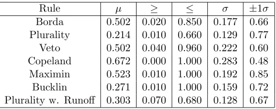
Rule µ ≥ ≤ σ ±1σ
Borda 0.502 0.020 0.850 0.177 0.66 Plurality 0.214 0.010 0.660 0.129 0.77 Veto 0.502 0.040 0.960 0.222 0.60 Copeland 0.672 0.000 1.000 0.283 0.48 Maximin 0.523 0.010 1.000 0.192 0.85 Bucklin 0.271 0.010 1.000 0.159 0.72 Plurality w. Runoff 0.303 0.070 0.680 0.128 0.67
Table 4.2: Arbitrary reordering robustness results for adversarial elections with 100 faults each. The mean is denoted byµ, the minimum and maximum
over all data points by≥and≤, standard deviation byσ, and percent within
[image:40.612.164.449.438.551.2]4.3
Results for Elementary Transposition
For the purposes of comparison with previous work, for which no experimen-tal data is available, we also conducted experiments using a single elemen-tary transposition as the type of noise, rather than the arbitrary reordering. The parameters are all identical to the experiments above, but with a single randomly-placed transposition in the preference profile. The results can be found in Table 4.3 for random profiles and Table 4.4 for adversarial profiles.
Rule µ ≥ ≤ σ ±1σ
[image:41.612.163.449.258.370.2]Borda 0.984 0.290 1.000 0.070 0.94 Plurality 0.985 0.610 1.000 0.036 0.93 Veto 0.986 0.660 1.000 0.033 0.92 Copeland 0.987 0.390 1.000 0.037 0.93 Maximin 0.994 0.390 1.000 0.024 0.95 Bucklin 0.985 0.610 1.000 0.036 0.93 Plurality w. Runoff 0.984 0.570 1.000 0.037 0.92
Table 4.3: Elementary transposition robustness results for random elections with 100 faults each. The mean is denoted byµ, the minimum and maximum
over all data points by≥and≤, standard deviation byσ, and percent within
one standard deviation by±1σ.
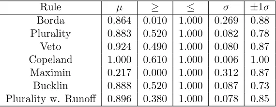
Rule µ ≥ ≤ σ ±1σ
Borda 0.864 0.010 1.000 0.269 0.88 Plurality 0.883 0.520 1.000 0.082 0.78 Veto 0.924 0.490 1.000 0.080 0.87 Copeland 1.000 0.610 1.000 0.006 1.00 Maximin 0.217 0.000 1.000 0.312 0.87 Bucklin 0.888 0.520 1.000 0.087 0.73 Plurality w. Runoff 0.896 0.380 1.000 0.078 0.85
Table 4.4: Elementary transposition robustness results for adversarial elec-tions with 100 faults each. The mean is denoted by µ, the minimum and
maximum over all data points by ≥ and ≤, standard deviation by σ, and
[image:41.612.163.448.453.564.2]Chapter 5
Conclusion
A summary of our research results on the bounds of robustness for arbitrary reordering, compared with the Procaccia et al. [27] results for elementary transpositions, can be found in Table 3.1. It is unsurprising to find that the bounds on robustness for some rules under arbitrary reordering are signifi-cantly worse than the Procaccia et al. bounds on elementary transpositions; however, it is certainly noteworthy that the upper bounds on Copeland and Maximin are actually better for arbitrary reordering than for elementary transposition. As discussed above in the section 3.2 definitions, an arbitrary