Simulating spatial and temporal evolution of multiple wing cracks around faults in
1
crystalline basement rocks
2 3
Jonathan P. Willson1, Rebecca J. Lunn2*, Zoe K. Shipton3 4
1
School of the Built Environment, Heriot-Watt University, Edinburgh, Scotland 5
2
Department of Civil Engineering, University of Strathclyde, Glasgow, Scotland 6
3
Department of Geographical and Earth Sciences, University of Glasgow, Scotland 7
8 9
Running title: Wing crack evolution around faults 10
Keywords: mechanical modeling, faults, splay fractures, damage zone, dynamic 11
Abstract
12
Faults zones are structurally highly spatially heterogeneous and hence extremely 13
complex. Observations of fluid flow through fault zones over several scales show that 14
this structural complexity is reflected in the hydrogeological properties of faults. 15
Information on faults at depth is scarce, hence, it is highly valuable to understand the 16
controls on spatial and temporal fault zone development. In this paper we increase our 17
understanding of fault damage zone development in crystalline rocks by dynamically 18
simulating the growth of single and multiple splay fractures produced from failure on a 19
pre-existing fault. We present a new simulation model, MOPEDZ, that simulates fault 20
evolution through solution of Navier’s equation with a combined Mohr-Coulomb and 21
tensile failure criteria. Simulations suggest that location, frequency, mode of failure and 22
orientation of splay fractures are significantly affected both by the orientation of the fault 23
with respect to the maximum principal compressive stress and the conditions of 24
differential stress. Model predictions compare well with published field outcrop data, 25
confirming that this model produces realistic damage zone geometries. 26
Introduction
29
Faults are structurally highly spatially heterogeneous and hence extremely complex 30
[Aydin, 2000; Caine et al., 1996; do Nascimento et al., 2005; Fairley and Hinds, 2004; 31
Galli et al., 2004; Wibberley and Shimamoto, 2003]. Observations of spatially 32
heterogeneous fluid flow through fault zones over several scales e.g. [do Nascimento et 33
al., 2005; Fairley and Hinds, 2004] show that this structural complexity is reflected in the 34
hydrogeological properties of faults. Within crystalline basement rocks, permeable faults 35
are a dominant feature of subsurface flow systems. The dominant deformation structures 36
in these systems are fractures that may be open or filled with minerals or gouge. Recent 37
research at the European Union’s Soultz-sous-Forêt Hot Dr y Rock test site [Evans et al., 38
2005a], underlines the importance of characterising fault zones. Data taken from low 39
pressure injection tests on the open borehole at Soultz show that almost all flow occurs 40
within a single fault zone located at 3490 m depth, and that just 10 major open fractures 41
account for 95% of the flow. 42
43
Fault zone structure can also vary temporally due to continued movement on the fault 44
and/or changing stress conditions. This can result in the creation of new fractures and the 45
reopening of sealed existing fractures, both of which may lead to increased fault zone 46
permeability. Observations during the high pressure injection tests at the HDR Soultz-47
sous-Forêt site confirm this link between fault damage zone evolution and increased flow 48
to the borehole [Evans, 2005; Evans et al., 2005b; Evans et al., 2005c]). Temporal 49
changes in fault hydraulic properties have also been observed in the hydrocarbon industry 50
52
The inaccessibility of subsurface faults, in combination with their spatial and temporal 53
complexity, makes it hard either to assess fault architectural structure or to predict fault 54
permeability. Data from boreholes and seismic surveys are available, however neither 55
provide the information necessary to constrain values of fault permeability. Given the 56
scarcity of information on faults at depth, it is advantageous to gain as much knowledge 57
as possible on the processes that govern spatial and temporal fault zone development. 58
Ultimately, if these processes can be numerically simulated, then predicted fault zone 59
architectures can be up-scaled to provide statistical estimates of bulk permeability fields. 60
The aim of our research is to predict damage zone features on small (subseismic) faults 61
with geometries that are geologically realistic. It is particularly important for estimation 62
of bulk fault permeability in crystalline rocks to accurately simulate the orientation and 63
connected nature of evolving fractures. In this paper, we present the first stage in 64
achieving this aim; simulating the dynamic growth of single and multiple splay fractures 65
produced from failure on pre-existing faults or joints. 66
67
Previous simulation studies of fault damage zone development 68
A number of researchers have employed numerical simulation methods to predict the 69
evolution of damage zone features surrounding faults. The modeling studies of 70
[Burgmann et al., 1994; Du and Aydin, 1993; 1995] employ Linear Elastic Fracture 71
Mechanics, first presented in [Pollard and Segall, 1987], to simulate the growth of splay 72
fractures from original faults or joints. [Du and Aydin, 1995] calculate the distribution of 73
and fault bends, and infer the directions of propagating fractures from the direction of 75
maximum distortional strain energy. [Shen and Stephansson, 1993] simulate the 76
propagation of shear fractures using the F-criteria based on combining the Maximum 77
Principal Stress and the Maximum Strain Energy Release Rate criteria, which they 78
propose for simulation of Mode I and Mode II fractures. Using the F-criteria, they 79
simulate damage at the fault tips whereby an initial single high angle tension fracture 80
evolves followed by a single shear fracture that propagates in the same direction as the 81
original fault. 82
83
More recently, research has focused on simulation of fault zone damage from dynamic 84
fault rupture in seismically active faults to improve estimates of energy losses during 85
earthquakes. [Yamashita, 2000] combines laboratory experiments with numerical 86
simulation to predict the generation of microcracks during macroscopic shear rupture. He 87
simulates the temporal evolution of maximum tensile stress at a rupture tip to infer the 88
location and orientation of associated microcracks in the surrounding rock. He concludes 89
that dynamically propagating earthquake faults generate a large number of tensile 90
microcracks in the surrounding fault zone. [Dalguer et al., 2003] develop and apply a 3D 91
Discrete Element Model to simulate crack propagation during the seismic rupture of a 92
pre-existing fault. They simulate the generation of new cracks within the surrounding 93
fault zone caused by progression of a single rupture patch on the fault with a tensile 94
failure criterion: as the rupture front progresses, tensile cracks expand and new cracks are 95
generated at the tip of the dynamic rupture patch. 96
In this paper we extend fault zone modeling of fault growth, such as that by [Burgmann et 98
al., 1994; Du and Aydin, 1993; 1995; Shen and Stephansson, 1993], to include spatial and 99
temporal evolution of single and multiple wing cracks within a fault damage zone in 100
crystalline basement. The model presented here introduces several novel processes that 101
have not been previously accounted for: cracks are propagated dynamically based on the 102
temporally evolving stress field; simulations investigate progressive microscopic-to-103
macroscopic failure; the model uses a combined Mohr Coulomb and tensile failure 104
criterion that allows for both shear and tensile failure of the rock. 105
106
Formulation of a Numerical Model for the Evolution of Fault Damage Zones
107
This paper presents a new model for the simulation of fault damage zone evolution. The 108
code is a two-dimensional coupled hydro-mechanical model, MOPEDZ (Modelling Of 109
Permeability Evolution in the Damage Zone surrounding faults), and is based on a finite 110
element approach to solving Navier’s equation with a combined Mohr Coulomb-tensile 111
failure criterion, coupled to the groundwater flow equation [Willson et al., 2005]. We 112
present the results of simulations using the mechanical modeling component of MOPEDZ 113
in order to investigate the controls on the evolution of wing crack generation around a 114
single pre-existing fault. 115
116
Navier’s equation is well known as describing the displacement of a body subject to 117
external forcing. The steady-state form of the equation can be written as 118
c
∇ ⋅ ∇ =u F (1)
Where F is the vector of external forces, u is a vector describing displacement and c is a 120
matrix where each entry is a function of the first and second Lamé constants. The failure 121
criteria employed to simulate rock fracturing in MOPEDZ are the Mohr-Coulomb and 122
tensile failure criteria, generally written as 123
(
)
[
]
32 2 1 2 0
1 µ 1 µ σ
σ ≤C + + + and σ3 ≤ −T0 (2)
124
respectively, where 1 is the maximum principal compressive stress, 3 is the minimum 125
principal compressive stress, C0 is the uniaxial compressive strength, is the coefficient 126
of friction and T0 is the tensile strength. 127
128
MOPEDZ is built using the commercially available finite element software, FEMLAB 129
[COMSOL, 2004]. FEMLAB is used to provide finite element subroutines that are called 130
from the MOPEDZ code, which has been developed, and is executed, within MATLAB. 131
MOPEDZ models the propagation of fractures by solution of Navier’s equation. Failure 132
is predicted by a combined Mohr-Coulomb and tensile failure criterion, which results in 133
changes to the material parameters at failed locations. Elements that contain fractures (as 134
opposed to intact host rock only) are represented by a reduction in the values of Young’s 135
Modulus, Poisson’s ratio and the material strength. This approach is similar to that of 136
[Tang, 1997] which has been successfully applied to simulate laboratory experiments and 137
reproduce fracture patterns around tunnels and boreholes. 138
139
The aim of MOPEDZ is to reproduce the change in material properties (Young’s 140
Modulus, Poisson’s ratio and the material strength) of a rock as it fails i.e. the first failure 141
spontaneously because of stress redistribution around previous failures. These subsequent 143
failures can be adjacent to previous failures, i.e. the extension of a fracture, or they can 144
occur in locations that are disconnected from any previous failure, but fail because of the 145
redistribution of stress. MOPEDZ solves Navier’s equation as a progressive series of 146
steady-states. Initially, the top and bottom boundaries of the model domain are displaced 147
inwards by a small increment. Navier’s equation is then solved and the number of 148
predicted failures examined. The displacement increment is then adjusted, and Navier’s 149
equation re-solved, such that a pre-defined small number of elements are predicted to fail, 150
resulting in a reduction in material properties for those elements. This approach of 151
numerically representing fracturing of an element of rock by reducing its material 152
properties was first developed and validated in rock mechanics using laboratory data 153
[Tang, 1997]. After the material properties have been reduced within MOPEDZ, Navier’s 154
equation is resolved (with no further boundary displacement). If elements are still 155
predicted to fail, the same process is repeated until no more failure is predicted i.e. a 156
steady-state is reached. Once a steady-state solution has been achieved for a given 157
boundary displacement, the boundaries are once more displaced to produce further shear 158
damage and the whole solution process is repeated. 159
160
The restriction of only a few elements for failure within each iterative solution ensures 161
stability of the model solution and a temporal propagation of cracks upon failure. For all 162
the simulations presented here, the number of failures for a single boundary displacement 163
failures were selected as it produced results almost identical to those allowing only a 165
single failure with each iteration. 166
167
Results
168
Figure 1 shows the temporal evolution of damage for a pre-existing fault with an 169
orientation of 30û to the maximum principal stress. In all simulations presented in this 170
paper, the maximum principal stress is orientated along the y-axis (i.e. top-to-bottom). 171
The accompanying simulation parameters (Table 1) are based on available laboratory 172
data for granite. In this simulation, σ3=0 on the lateral boundaries of the model and the 173
top and bottom boundaries are gradually displaced inwards as described above. Note that 174
the position of the pre-existing fault is non-central, with the fault being located slightly to 175
the right hand side of the domain. Figure 1 shows progressive temporal development of a 176
single splay fracture, formed under tension, propagating from each end of the fault at an 177
angle of 70û measured anticlockwise from the plane of the fault. Due to the asymmetry of 178
the fault in the domain, damage progresses more rapidly at the upper fault tip. 179
Simulations (not shown here) with a central fault predict the evolution of symmetric 180
damage zone structures. The results in Figure 1 are in keeping with LEFM, with the final 181
structure being similar to that in Figure 7a of [Burgmann et al., 1994] where tensile wing 182
cracks are predicted (using a steady-state model) to initiate at 70û with a boundary 183
condition of a prescribed shear force applied to the pre-existing fault. 184
185
Figure 1 demonstrates that MOPEDZ can predict the evolution of fault zone structures 186
MOPEDZ to explore temporal damage zone evolution under differing conceptual 188
scenarios. We investigate for the first time, the effects on temporal and spatial damage 189
zone evolution of: progressive breakdown of the rock; the magnitude and orientation of 190
the confining stress; the host rock heterogeneity. 191
192
How Does Damage to Rocks Progressively Occur? 193
The method by which the material properties of a finite element should be changed as it 194
becomes progressively more fractured is dependent on the how the process of fracturing 195
is conceptualized i.e. the micro-scale processes that represent different bulk weakening 196
behaviors. There are two possible scenarios for the failure process within the elements. 197
The first scenario is that upon failure, a single fracture occurs that spans the whole 198
element, and subsequent failure produces either further smaller fractures that propagate 199
off this fracture or increases the aperture on the original fracture, resulting in progressive 200
weakening of the element (Figure 2a). The second scenario is that when the confining 201
stress is sufficiently high, many locations fail within the element, producing a large 202
number of microfractures. Further stress increases cause the microfractures to eventually 203
coalesce and a single main fracture dominates and spans the whole of the element (Figure 204
2b). Scenario 1 is equivalent to a large drop in strength followed by progressive 205
continued strength breakdown (infilling with weak minerals [Niemeijer and Spiers, 2005] 206
or absorption of water into fault gouge [Morrow et al., 2000]). Scenario 2 would 207
correspond to progressive strength breakdown followed by a large drop in strength. This 208
would be equivalent to the process zone model for fracture growth [Lockner et al., 1992]. 209
for an element that represents both microscopic damage and a through-going fracture 211
(See final frames of Figure 2). 212
213
To reproduce the above scenarios, MOPEDZ simulations were conducted, again using the 214
parameter values in Table 1, but allowing for a progressive reduction in Young’s 215
modulus on a failed element. The first scenario above assumes that most damage occurs 216
in the first failure followed by smaller subsequent failures. This can be expressed as a 217
geometric series, relating the value of the material parameter of interest, Dn, after failure,
218
to the previous value of that material parameter, Dn-1
219 m n D M M D n m hr f
n 1 where 1,2,...,
1 = ⎟⎟ ⎠ ⎞ ⎜⎜ ⎝ ⎛
= − (2)
220
where Mf is a constant representing the lowest possible value of the material parameter
221
for a completely fractured element, Mhr is the value of the material parameter
222
representing intact host rock, m is the number of levels of progressive damage, and D0 is
223
equal to Mhr.
224 225
In the second scenario, microfracturing occurs first, followed by macroscopic failure. In 226
this case, the relative reductions in the above series were reversed to produce small initial 227
reductions in material properties followed by progressively larger ones. Results for these 228
two scenarios allowing a total of three progressive failures of a single element (i.e. m=3) 229
are shown in Figure 3(a) and (b). In the case of initial microfracturing followed by 230
macroscopic failure (i.e. the second scenario above) a single tensile fracture evolves at 231
element, multiple parallel tensile fractures are observed (Figure 3b). The first fracture to 233
evolve is the longest fracture, at the tip, with subsequent fractures evolving progressively 234
toward the centre of the fault. Fracture length decreases linearly toward the centre of the 235
fault. 236
237
To investigate the role of mesh refinement on the development and location of the 238
multiple splay fractures predicted in Figure 3(b), a further simulation was conducted 239
using a finer mesh. Figure 3(c) shows results from a simulation identical to that in Figure 240
3(b) but with a 160 × 160 mesh i.e. four times the number of elements (this was the limit 241
of the virtual memory available within MATLAB). The preexisting fault for the finer 242
mesh has the same physical thickness as that in the 80×80 case, although its diagonal 243
representation within the square mesh results in a smoother pixelisation of the fault 244
surface. A comparison of Figures 3(b) and (c) shows the results to very similar, both 245
simulations produce parallel splay fractures that decrease in length toward the centre of 246
the fault. In Figure 3c, the finer mesh allows these splays to appear slightly earlier in the 247
simulation and to be closer together, hence they are more concentrated toward the fault 248
tip. Further simulations not shown here, using an even finer adaptive triangular mesh to 249
represent a completely smooth initial fault surface, with an increased length to width ratio 250
(a thinner fault), also produced results similar to those in Figure 3(c): the cracks 251
concentrate at the fault tip and are slightly shorter relative to the length of the original 252
fault. In summary, Figures 3(b) and (c) show that the basic geometry of the results 253
and more concentrated at the fault tip, this is consistent with observations of multiple 255
splay fractures in the field (see discussion and Figure 8a). 256
257
In all subsequent simulations within this paper, the first scenario of immediate 258
macroscopic fracturing, followed by progressive but decreasing weakening, is adopted to 259
investigate the evolution of multiple splay fractures in fault damage zones. This allows 260
for investigation of differing mechanical phenomena to those presented by previous 261
authors such as [Du and Aydin, 1995; Shen and Stephansson, 1993]. For computational 262
feasibility, the mesh resolution in the following sections is 80×80 which enabled multiple 263
simulations to be performed within a reasonable time scale. 264
265
How are Fault Damage Zone Structures Influenced by the Confining Stress? 266
To investigate the role of confining stress in influencing the damage surrounding faults, 267
four different cases were investigated. The final structures obtained for each of these 268
cases are presented in Figure 4. In Figure 4(a) 3 = 0. Figure 4(b) shows results for the 269
same simulation but with 1/ 3 = 5. In this simulation multiple parallel tension cracks are 270
again produced, but here the longest splay fracture is not now associated with the fault 271
tip. In Figure 4(c), the final damage zone structure is shown for 1/ 3 = 2.5. Now a 272
different pattern of damage is observed: wing cracks evolve due to shear failure at the 273
fault tips and propagate at a much lower angle to the original fault plane. In addition to 274
these shear cracks, small tensional cracks form at a higher orientation to the fault and 275
away from the fault tip. In the final simulation (Figure 4d) the boundaries are completely 276
perpendicular tertiary fractures then propagate from these shear fractures. The same 278
structures as those in Figure 4(d) were produced as 1/ 3 tended to a value of one (i.e. 279
1 3). The results in Figure 4 imply that for large differential stress (i.e. 1» 3) 280
multiple parallel tension fractures are formed, whereas for small differential stress ( 1 281
close to 3) single shear fractures form at the fault tip followed by small higher angle 282
tension fractures. 283
284
The effect of varying the orientation of the maximum principal stress with respect to the 285
pre-existing fault is examined in Figure 5. Simulations were conducted for faults at 286
angles of 30û, 45û, 60û and 75û to 1 for the two extreme cases in Figure 4 of 3 = 0 and of 287
rigid lateral boundaries, from here termed high and low differential stress respectively. 288
For high differential stress (Figure 5a) all wing cracks form in tension and ultimately 289
propagate in the direction of the maximum principal stress. Figure 5a shows that faults at 290
low angles to the maximum principal stress (30û and 45û) produce single curved splay 291
fractures. As the angle between the fault and 1 increases, multiple parallel fractures 292
evolve that decrease in length toward the centre of the fault. Once the fault is oriented at 293
75û to 1 the geometry of the fracturing becomes more erratic, splay fractures evolve on 294
both sides of the fault at the same tip, and there is no clear pattern to fracture length. In 295
the case of low differential stress (Figure 5b) the predicted damage zone structures are 296
very different. For a fault at an angle of 30û to 1, wing cracks form in shear and 297
propagate back into the compressive quadrant. As the angle increases, shear fractures 298
angles, short tension fractures also form away from the fault tip at an angle of 85û to the 300
original fault. 301
302
Does Host Rock Heterogeneity Affect Damage Zone Formation? 303
To explore the effect of host rock heterogeneity, simulations were conducted using both 304
purely random and spatially correlated fields for host rock material properties. Six 305
realizations were simulated for each statistical material property distribution, in 306
conditions of high differential stress. Final damage zone structures for two of the 307
realizations of the host rock material properties in each case are shown in Figure 6. 308
Figure 6 (row 1) shows final damage zone structures for an uncorrelated, purely random 309
field where the mean Young’s modulus of the host rock is 60 GPa (as on previous 310
simulations) with a standard deviation of 1 GPa (i.e. 95% of the field lies between 58GPa 311
and 62 GPa). For comparison, a completely fractured element is represented by a 312
Young’s modulus of 1.2 GPa, so the original fault remains quite distinct from any 313
underlying variations in the host rock. Visual inspection of the simulations in Figure 6 314
row 1 shows that both realizations produce multiple parallel splay fractures, but in the 315
first realization a splay fracture forms beyond the fault tip. 316
317
Figure 6, rows 2 to 4, show the results of simulations identical to those in row 1 but with 318
a host rock Young’s modulus that is described by a spatially correlated random field. The 319
covariance structure of this field is described by an exponential function of the form 320
(
λ)
σ h
h
C( )= 2 −exp − (4)
where is the termed the correlation length and effectively governs the size of the 322
‘patches’ of high or low Young’s modulus in the host rock, 2 is the variance and h is the 323
distance between pairs of points in the field. The results for the final damage zone 324
structure for 3 different correlation lengths are shown in Figure 6 (rows 2 to 4) two 325
realizations are shown for each different correlation length. Again, multiple parallel splay 326
fractures are produced with some of these forming beyond the fault tip. Realizations with 327
high numbers of parallel fractures correspond to those with patches of low host rock 328
Young’s modulus adjacent to the fault. For the simulation with the largest correlation 329
length, a shear fracture can be seen propagating from the left hand fault tip. It is clear that 330
whilst the macroscopic damage zone pattern remains very similar in these simulations, 331
the exact locations and frequencies of evolving splay fractures are heavily influenced by 332
the heterogeneous material properties of the host rock. 333
Discussion
335
The simulation results presented here have investigated the formation of fractures around 336
a single pre-existing feature (described here as a fault, but which could represent other 337
pre-existing features such as joints and dikes [d'Alessio and Martel, 2005]). We have 338
investigated varying the effect of: the conceptual scenario of progressive fracture 339
damage; the orientation of the initial fault with respect to the maximum principal 340
compressive stress; the confining boundary conditions; and the heterogeneity of the host 341
rock material properties. The range of resulting damage zone structural styles are 342
summarized in Figure 7. Typical structures are a) single tensile wing cracks, b) multiple 343
tensile wing cracks, c) unconnected tensile fractures, d) low angle wing cracks that have 344
formed in shear e) low angle shear cracks with tertiary fractures subsequently 345
propagating off their sides, and f) high angle shear fractures that propagate at angles 346
between 180º and 270º (measured anticlockwise from the original fault plane). 347
Interestingly, one key form of damage zone evolution that is not predicted here is an 348
extension of the initial fault in its own plane. Fault plane extension has been previously 349
simulated by [Du and Aydin, 1993; 1995], however, in their conceptual model of 350
mechanical failure, tensile failure is suppressed. 351
352
Comparison with previous theory and outcrop measurements. 353
This research has produced tensile wing cracks that vary in angle from 30º to 90º and 354
synthetic shear wing cracks that vary from 23º to 40º. This range is far broader than the 355
range predicted by Linear Elastic Fracture Mechanics [Pollard and Segall, 1987] which 356
358
Wing crack measurements on outcrops are generally low, but can range from 15º to 70º. 359
The angles produced by MOPEDZ compare well with field observation of wing crack 360
angles (Table 2). In our simulations, the most influential factor is the orientation of the 361
fault relative to the maximum principal stress direction. Since faults in crystalline rocks 362
are generally thought to evolve from the linking of pre-existing joints [Martel, 1990] or 363
dikes [d'Alessio and Martel, 2004], the maximum principal stress direction must have 364
originally been aligned with their pre-existing structures. It seems reasonable to presume 365
that smaller rotations of the stress field will be more common than larger ones, and this 366
would result in wing cracks frequently occurring at angles at the lower end of the possible 367
range. 368
369
For a comparison of MOPEDZ with field observations, Figure 8a shows a 14m long fault 370
developed in granodiorite in the Kip Camp area of the Sierra Nevada, California mapped 371
by [Lim, 1998]. The length of the wing cracks in Figure 8a is related to distance from the 372
fault tip, with a general decrease in length of the wing cracks as the distance from the 373
fault tip increases. The adjacent MOPEDZ simulation shown compares well with the type 374
of damage shown in [Lim, 1998]. The simulation has high differential stress (i.e. σ1»σ3) 375
assumes immediate macroscopic damage of the host rock on initial failure, and has a fault 376
inclined at 60º to the maximum principal compressive stress. The simulation produces 377
wing cracks that propagate at around 60º, that are distributed along the length of the joint 378
and that decrease in length as the distance from the tip increases. This simulation suggests 379
the direction of the maximum principal stress for the fault in Figure 8a was 381
approximately north-south. 382
383
Figure 8b shows the Alligerville fault, New York state, mapped by Vermilye & Scholz 384
[1998]. The 40m long vertical fault is in quartzite [Vermilye & Scholz 1998]. The fault 385
has shear wing cracks that propagate in the compressional quadrants at angles of around 386
225º, which are distributed along the length of the fault, and decrease in length as the 387
distance from the fault tip increases. The fault also shows pressure solution cleavage in 388
the compressional quadrant, striking at approximately -60º. The adjacent MOPEDZ 389
simulation shown in Figure 8b compares well with the Alligerville fault trace. This 390
simulation has confined boundary conditions, assumes immediate macroscopic damage 391
of the host rock on initial failure (Figure 3a) and has an initial fault orientation of 30º to 392
the maximum principal compressive stress. The simulation produces shear wing cracks 393
that propagate from the fault tips into the compressional quadrant at around 242º . In the 394
Alligerville fault, multiple fractures are formed which are not reproduced in the 395
MOPEDZ simulations, this may be due to the heterogeneity of the host rock, or due to the 396
clear deviations from a planar fault surface (which would concentrate stress) that are 397
apparent on the Alligerville fault. Based on our simulations, we suggest that the direction 398
of the maximum principal stress around the Alligerville fault was approximately north-399
west/south-east when fracturing developed, and that the differential stress was low. 400
Implications for the temporal sequence of multiple wing cracks. 402
A number of conceptual temporal sequences for the evolution of multiple splay fractures 403
have been proposed e.g. [Martel and Pollard, 1989]. Four conceptual temporal sequences 404
(S1 to S4) are possible (Figure 9). In S1, wing cracks form behind (i.e. away from) the 405
fault tip, and then further wing cracks form progressively nearer to the fault tip (Figure 406
9a); this is essentially the sequence proposed in [Martel and Pollard, 1989] and simulated 407
for seismic rupture in [Dalguer et al., 2003]. In S2, wing cracks form initially at the tips 408
of the fault and then further wing cracks form at locations that are progressively closer to 409
the middle of the joint (Figure 9b). In S3, wing cracks form at the tips, subsequently the 410
fault extends in its original plane, and then further wing cracks form at the new tips 411
(Figure 9c). Finally in S4, wing cracks form at the tips of the fault, parallel wing cracks 412
form that are away from and unconnected to the fault tip, the tip then extends and 413
connects to these parallel cracks (Figure 9d) . 414
415
Based on the simulations presented here, the most likely sequence for temporal evolution 416
is that of S2 (Figure 9b). Almost all MOPEDZ simulations predict the first wing crack to 417
occur at the fault tip. In general, further wing cracks then form progressively further 418
away from the tip toward the centre of the fault. This temporal sequence matches that of 419
S2 in Figure 9b. However, in simulations with low differential stress and an angle of at 420
least 75û to the maximum principal compressive stress the first wing cracks are predicted 421
to initiate away from the fault tip (S1, Figure 9a). For these high angle faults, the 422
formation of wing cracks is predicted to be highly irregular in length, with a few cracks 423
Finally, in a few of the realizations incorporating a fault within a heterogeneous host 425
rock, fractures occur beyond the tip of the fault without any extension of the original fault 426
in its own plane. Once these fractures have formed it is possible that subsequent 427
fracturing could link these off-tip fractures (sequence S4, Figure 9d) but this final linking 428
stage has not been produced here. 429
430
Implications for fluid flow 431
The future application of physically-based simulation models to improve estimates of 432
fault hydraulic properties in the subsurface, depends critically on being able to accurately 433
predict the orientation, frequency and connected nature of evolving fractures in the 434
damage zone. In this paper, we demonstrate that it is possible to simulate the spatial and 435
temporal evolution of multiple splay fractures from a single pre-existing fault. 436
Simulations are compared with field observation data and the orientation of the predicted 437
fractures compares well with observed fault zone geometries. The model can now 438
confidently be applied to investigate more complex fault zone geometries, such as fault 439
zone development from linkage of pre-existing joints [Martel, 1990], and combined with 440
fluid flow simulation [Willson et al., 2005] for bulk permeability estimation. 441
442
Conclusions
443
We present a new model, MOPEDZ, for dynamic simulation of multiple and single splay 444
fractures originating from a single feature such as a fault, joint or dike. The model is 445
based on a finite element solution of Navier’s equation using a combined Mohr-Coulomb 446
zone geometry. Investigations of damage zone evolution under differing boundary 448
conditions and material properties predict that: 449
• Changing the conceptual sequence of microscopic versus macroscopic fracturing 450
of an element results in important differences in the structure of the damage zone 451
around slipping faults. Simulations show that a conceptual sequence of 452
microscopic damage followed by macroscopic failure tends to produce single 453
splay fractures at the fault tip, whereas immediate macroscopic failure produces 454
multiple parallel splay fractures that decrease in length away from the fault tip. 455
• Due to the combined Mohr Coulomb and tensile failure criteria, which allows 456
both shear and tensile failure, the orientations of damage zone features 457
surrounding the fault are heavily influenced by the differential stress. For low 458
differential stress, simulations predict single shear fractures at the fault tip that 459
propagate at a low angle to the fault. For high differential stress,, fractures form in 460
tension at the fault tips followed by multiple parallel fractures that are 461
progressively closer to the fault centre and shorter in length. 462
• Faults that are reactivated at a high angle to the maximum principal compressive 463
stress form multiple parallel splay fractures. By comparison, faults at a low angle 464
to the maximum principal stress, form single fractures at the fault tips. For 465
simulations where the differential stress is low, these single fractures propagate 466
into the compressional quadrant. 467
• Host rock heterogeneity effects the locations of evolving splay fractures 468
• In the case of multiple splay fractures, simulations generally support a temporal 470
evolution in which the initial fracture occurs at the fault tip. This is then followed 471
by the evolution of other parallel features that are progressively both shorter in 472
Acknowledgements
References List
Anderson, R. N., P. Flemings, S. Losh, J. Austin, and R. Woodhams (1994), Gulf-of-Mexico Growth Fault Drilled, Seen as Oil, Gas Migration Pathway, Oil & Gas Journal, 92(23), 97-104.
Aydin, A. (2000), Fractures, faults and hydrocarbon entrapment migration and flow, Marine and Petroleum Geology, 17, 797-814.
Burgmann, R., D. D. Pollard, and S. J. Martel (1994), Slip distributions on faults: effects of stress gradients, inelastic deformation, heterogeneous host-rock stiffness, and fault interaction, Journal of Structural Geology, 16(12), 1675-1690.
Byerlee, J. D. (1967), Frictional characteristics of granite under high confining pressure., Journal of Geophysical Research, 72, 3639-3648.
Caine, J. S., J. P. Evans, and C. B. Forster (1996), Fault zone architecture and permeability structure, Geology, 24(11), 1025-1028.
COMSOL (2004), FEMLAB, edited, COMSOL AB.
Cruikshank, K. M., G. Zhao, and A. M. Johnson (1991), Analysis of minor fractures associated with joints and faulted joints, Journal of Structural Geology, 13(8), 865-886. d'Alessio, M. A., and S. J. Martel (2004), Fault terminations and barriers to fault growth, Journal of Structural Geology, 26, 1885-1896.
d'Alessio, M. A., and S. J. Martel (2005), Development of strike-slip faults from dikes, Sequoia National Park, California, Journal of structural geology, 27(1), 35-49.
Dalguer, L. A., K. Irikura, and J. D. Riera (2003), Simulation of tensile crack generation by three-dimensional dynamic shear rupture propagation during an earthquake, J. Geophys. Res.-Solid Earth, 108(B3).
do Nascimento, A. F., R. J. Lunn, and P. A. Cowie (2005), Modeling the heterogeneous hydraulic properties of faults using constraints from reservoir-induced seismicity, J. Geophys. Res.-Solid Earth, 110(B9).
Du, Y. J., and A. Aydin (1993), The Maximum Distortional Strain-Energy Density Criterion for Shear Fracture Propagation with Applications to the Growth Paths of En-Echelon Faults, Geophysical Research Letters, 20(11), 1091-1094.
Du, Y. J., and A. Aydin (1995), Shear Fracture Patterns and Connectivity at Geometric Complexities Along Strike-Slip Faults, J. Geophys. Res.-Solid Earth, 100(B9), 18093-18102.
Evans, K. F. (2005), Permeability creation and damage due to massive fluid injections into granite at 3.5 km at Soultz: 2. Critical stress and fracture strength, J. Geophys. Res.-Solid Earth, 110(B4).
Evans, K. F., A. Genter, and J. Sausse (2005a), Permeability creation and damage due to massive fluid injections into granite at 3.5 km at Soultz: 1. Borehole observations, Journal of Geophysical Research, 110(B04203).
Evans, K. F., A. Genter, and J. Sausse (2005b), Permeability creation and damage due to massive fluid injections into granite at 3.5 km at Soultz: 1. Borehole observations, J. Geophys. Res.-Solid Earth, 110(B4).
Evans, K. F., H. Moriya, H. Niitsuma, R. H. Jones, W. S. Phillips, A. Genter, J. Sausse, R. Jung, and R. Baria (2005c), Microseismicity and permeability enhancement of
Fairley, J. P., and J. J. Hinds (2004), Rapid transport pathways for geothermal fluids in an active Great Basin fault zone, Geology, 32(9), 825-828.
Galli, G., A. Grimaldi, and A. Leonardi (2004), Three-dimensional modelling of tunnel excavation and lining, Computers and Geotechnics, 31(3), 171-183.
Lim (1998), Small strike slip faults in granitic rock: implications for three-dimensional models, Masters Thesis thesis, Utah State University, Logan, Utah.
Lockner, D. A., J. D. Byerlee, V. Kuksenko, A. Ponomarev, and A. Sidorin (1992), Observations of quasistatic fault growth from acoustic emissions, in Fault mechanics and transport properties of rocks, edited by B. Evans and T.-F. Wong, pp. 1-31, Academic Press, San Francisco.
Losh, S. (1998), Oil Migration in a Major Growth Fault: Structural Analysis of the Pathfinder Core, South Eugene Island Block 330 Field, Offshore Louisiana, AAPG Bulletin, 82(9), 1694-1710.
Losh, S. (2006), Episodic fluid flow and aseismic slip, AGU Monograph.
Martel, S. J., and D. D. Pollard (1989), Mechanics of Slip and Fracture Along Small Faults and Simple Strike-Slip-Fault Zones in Granitic Rock, Journal of Geophysical Research-Solid Earth and Planets, 94(B7), 9417-9428.
Martel, S. J. (1990), Formation of Compound Strike-Slip-Fault Zones, Mount Abbot Quadrangle, California, Journal of Structural Geology, 12(7), 869-&.
Martin, C. D. (1997), Seventeenth Canadian geotechnical colloquium: the effect of cohesion loss and stress path on brittle rock strength, Can Geotech Journal, 34(5), 698-725.
Morrow, C. A., D. E. Moore, and D. A. Lockner (2000), The effect of mineral bond strength and adsorbed water on fault gouge frictional strength, Geophysical Research Letters, 27(6), 815-818.
Niemeijer, A. R., and C. J. Spiers (2005), Influence of phyllosilicates on fault strength in the brittle-ductile transition: Insights from rock analogue experiments, paper presented at High-strain zones: Structure and physical properties, Geological Society of London Special Publications.
Pollard, D. D., and P. Segall (1987), Theoretical displacements and stresses near fractures in rock: with applications to faults, joints, veins, dykes and solution surfaces, in Fractals in the Earth Sciences, edited by A. B, pp. 89-105, Plenum Press New York.
Segall, P., and D. D. Pollard (1983), Nucleation and Growth of Strike Slip Faults in Granite, Journal of Geophysical Research, 88(NB1), 555-568.
Shen, B., and O. Stephansson (1993), Numerical-Analysis of Mixed Mode-I and Mode-Ii Fracture Propagation, Int. J. Rock Mech. Min. Sci., 30(7), 861-867.
Tang, C. A. (1997), Numerical Simulation of Progressive Rock Failure and Associated Seismicity, International Journal of Rock Mechanics and Mining Sciences, 34(2), 249-261.
Turcotte, D., and J. Schubert (1982), Geodynamics, 2nd Edition ed., Cambridge University Press, Cambridge.
Vermilye, J. M., and C. H. Scholz (1998), The process zone: A microstructural view of fault growth, J. Geophys. Res.-Solid Earth, 103(B6), 12223-12237.
Willson, J. P., R. J. Lunn, Z. K. Shipton, and P. A. Cowie (2005), Modelling hydraulic permeability evolution in fault damage zones, paper presented at EUROCK 05, A.T. Balkema & G. Westers, Brno.
Figure 1 Temporal development of wing cracks at the tips of a single fault, using the parameters listed in Table 1 and σ3=0. The maximum principal stress (σ1) is oriented top to bottom in these simulations. Each
frame shows the structure that has developed by increasing the boundary displacement, y, to the amount indicated. The grey scale represents material Young’s modulus; grey is unfractured (60GPa) and black is fractured (1.2GPa). The angle between the fault and the wing crack is measured anticlockwise from the plane of the fault
Figure 2 Sequences of progressive fracturing for a single finite element a) development of fracturing assumes that the major fracture happens first, and subsequent fractures are smaller (shown for three steps),
b) development of fracturing assumes that microfractures occur first, and larger fractures develop through coalescence of these fractures.
Figure 3 Temporal damage zone progression a) assuminginitial macroscopic failure with an 80×80 mesh (see Figure 2a) b) initial microscopic failure with an 80×80 mesh (see Figure 2b) c) assuming initial macroscopic failure with an 160×160 mesh (see Figure 2a) d) assuminginitial microscopic failure with an 160×160 mesh (see Figure 2b). The maximum principal stress (σ1) is oriented top to bottom.
Figure 4 Comparison of simulations with different ratios of σ1 to σ3.The maximum principal stress (σ1) is
oriented top to bottom. a) σ3 = 0 (this is a reproduction of the final damage structure in Figure 3a), b) a
ratio of σ1 / σ3 = 5, c) a ratio of σ1 / σ3 = 2.5, d) rigid left and right boundaries.
Figure 5 Resulting structures when varying fault orientation for a boundary displacement of approximately 6.8mm. The orientation between the fault and σ1 (oriented top to bottom) is 30º, 45º, 60º and 75º for a) high
differential stress and b) low differential stress.
Figure 6 Resulting structures using a heterogeneous Young’s modulus field for a boundary displacement of approximately 3mm. Each simulation starts with a different heterogeneous Young’s modulus matrix. The maximum principal stress (σ1) is oriented top to bottom. There are 2 realisations each of a purely random
field and of three different of correlation lengths of 0.15m, 0.375m and 0.45m. Colour scale is logarithmic and indicates Young’s modulus.
Figure 7 Six fault tip structural styles that have been produced with MOPEDZ.
Figure 8 a) A fault in granodiorite showing multiple wing cracks distributed along its entire length [Lim, 1998] alongside a structure produced by MOPEDZ with high differential stress starting with a fault inclined at 60º to the maximum principal stress. The mapped fault strikes at 57º and dips 81º to the south, the grey rectangle on the map indicates ground cover, and it is presumed the fault is continuous [Lim, 1998]. b)
Outcrop map of a fault after Vermilye & Scholz [1998] alongside a simulation produced by MOPEDZ with low differential stress, starting from a fault that is inclined at 30º to the maximum principal compressive stress
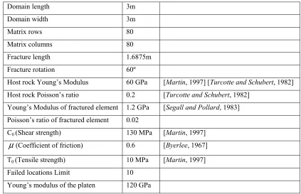
Domain length 3m
Domain width 3m
Matrix rows 80
Matrix columns 80
Fracture length 1.6875m
Fracture rotation 60º
Host rock Young’s Modulus 60 GPa [Martin, 1997] [Turcotte and Schubert, 1982]
Host rock Poisson’s ratio 0.2 [Turcotte and Schubert, 1982]
Young’s Modulus of fractured element 1.2 GPa [Segall and Pollard, 1983]
Poisson’s ratio of fractured element 0.02
C0 (Shear strength) 130 MPa [Martin, 1997]
µ(Coefficient of friction) 0.6 [Byerlee, 1967]
T0 (Tensile strength) 10 MPa [Martin, 1997]
Failed locations Limit 10
[image:29.612.80.503.97.370.2]Young’s modulus of the platen 120 GPa
Table 1 MOPEDZ simulation parameters, where relevant the right hand column contains the reference from which the value of the mechanical property for granite was derived
Author Range of wing
crack angles
Rock type and location
[Lim, 1998] 20º to 70º Granite, Sierra Nevada, California [Segall and Pollard, 1983] 15º to 35º Granite, Sierra Nevada, California [Cruikshank et al., 1991] 35º to 50º Sandstone, Arches National Park, Utah
[image:29.612.85.528.453.512.2]