Vibration-based damage detection in structures using time series analysis

using time series analysis. Proceedings of the Institution of Mechanical

Engineers, Part C: Journal of Mechanical Engineering Science, 220 (3).

pp. 261-272. ISSN 0954-4062 , http://dx.doi.org/10.1243/09544062C12904

This version is available at

https://strathprints.strath.ac.uk/5015/

Strathprints is designed to allow users to access the research output of the University of Strathclyde. Unless otherwise explicitly stated on the manuscript, Copyright © and Moral Rights for the papers on this site are retained by the individual authors and/or other copyright owners. Please check the manuscript for details of any other licences that may have been applied. You may not engage in further distribution of the material for any profitmaking activities or any commercial gain. You may freely distribute both the url (https://strathprints.strath.ac.uk/) and the content of this paper for research or private study, educational, or not-for-profit purposes without prior permission or charge.

Any correspondence concerning this service should be sent to the Strathprints administrator:

[email protected]

The Strathprints institutional repository (https://strathprints.strath.ac.uk) is a digital archive of University of Strathclyde research outputs. It has been developed to disseminate open access research outputs, expose data about those outputs, and enable the

Vibration-based damage detection in

structures using time series analysis

Department of Mechanical Engineering, University of Strathclyde, 75 Montrose Street, Glasgow G1 1XJ, UK. email: [email protected]

The manuscript was received on 20 July 2004 and was accepted after revision for publication on 10 November 2005.

DOI: 10.1243/09544062C12904

Abstract: The paper considers some possibilities to use pure time series analysis for damage diagnosis in vibrating structures. It introduces the basics of the state space methodology and discusses a number of possible methods to extract damage sensitive features from the state space representation of the attractor of a vibrating system. The discussed methods can be divided into two groups: methods that use non-linear dynamics characteristics and methods based on the statistical characteristics of the distribution of points on the attractor. Each possible damage feature is introduced separately and the advantages and shortfalls of its appli-cation are discussed. The appliappli-cation of the suggested techniques is demonstrated on a test case of a reinforced concrete plate.

Keywords: vibration-based structural health monitoring, linear time series analysis, non-linear dynamics, state space representation of dynamical systems, dynamic system invariants, dynamic system attractor

1 INTRODUCTION

Owners of structures – civil, mechanical, aircraft, marine, space – strive to extend their useful life while still maintaining them in safe operational con-ditions. The safety of most structures is another issue of vital importance: the collapse of a structure (civil, aircraft, bridge, power station) can be catastrophic in terms of casualties, environmental damage and losses. The development of new materials and tech-nologies has promoted significantly the former goals and the field of structural health monitoring has been developing rapidly during the last years to address the aforementioned goals.

Vibration-based damage detection methods are based on the fact that any change introduced in a structure results in changes in its dynamic beha-viour. Thus introduction of even a small damage will change the physical characteristics of a structure (its mass, stiffness, damping characteristics), which in turn will affect its vibration response and change its dynamic characteristics. Vibration-based damage detection methods are especially attractive because they are global monitoring methods in the sense that no a priori information for the location

of the damage is needed and/or immediate access to the damaged part is not required. These features are especially important when the objects of moni-toring are large and/or complex structures and when some parts of these structures are either inac-cessible or very difficult for taking measurements (buildings, bridges, offshore platforms).

number of modal-based and FRF-based methods is that they rely on a certain model of the structure. In most cases, these models are linear, while the majority of real structures exhibit non-linear beha-viour because of their material properties, geometry, non-linearities in the joints and the boundary conditions. Such methods will give a false alarm due to a discrepancy between the measured and the model response.

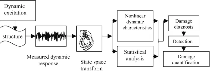
To address some of the afore-mentioned problems, a new paradigm has been emerging recently in vibration-based monitoring – the employment of the measured time series response of the structure. Techniques, which apply pure time series analysis will not necessarily suffer the above limitations and may provide a broader utility due to their generic approach. Time series analysis, which draws most of its applications from statistical analysis and non-linear dynamics, can provide a number of features and techniques that may hold significant promise for structural health monitoring. The state space approach provides the basis for most time series methods. It is known that any dynamic system can be completely recovered in a new state space, which may be reconstructed from the measured time domain response of the system [1]. A dynamic system can be characterized in different ways using its state space reconstruction. One way is to use its dimension and stability characteristics (non-linear dynamics characteristics). Another way is to study the statistical characteristics of the set of points that the system occupies in its state space. These two approaches are considered more or less identical because it has been proven that the second approach can also provide the non-linear dynamics character-istics of the system [2]. The problem for vibration-based structural health monitoring using the measured time series response of the structure can be schematically represented as shown in Fig. 1. Concerning the feature extraction phase of this approach, damage sensitive features can be

extracted either using the non-linear dynamics characteristics of the system or employing the stat-istical characteristics of its attractor in the state space.

Although time series analysis seems to hold a lot of potential for vibration-based monitoring, these methods remain more or less unexplored except for a couple of attempts [3–8]. The purpose of this paper is to offer several possible damage sensitive parameters based on time series analysis. Health monitoring methods based on such parameters would be more appropriate for large, complex, and especially non-linear structures which are particu-larly difficult to model. The suggested methods offer only a few possibilities to extract features from the state space representation of the structural response, and in this sense they are not in any way exhaustive: the approach as such seems to hold a considerable potential for the study of vibrating structures. The novelty and the contribution of this investigation are in the development and the adap-tation of the state space approach for structural damage detection purposes.

2 THE STATE SPACE APPROACH

The concept for state space representation and reconstruction stems from the dynamical system approach for analysis of non-linear time series. The main idea of this approach is to equip the investi-gator with tools for analysis and modelling of a system from observed time-dependent variables. Each dynamic system can be represented by a system of differential equations

dx

dt ¼F(x(t)) (1)

In most cases, the functionF(.) in the above model is not explicitly known and the original system space

defined by the vector x is also unknown. Any dynamic system can be completely unfolded in its state space, where the trajectories of the system con-verge to an invariant subspace (the attractor). The question is how to reconstruct this state space especially for cases when there is not enough a priori information available about the system and one is able to observe only one or two variables. Obviously a vibrating structure is a much more com-plex system and cannot be represented in a one-dimensional space. Takens theorem [1] gives the answer to this question. The theorem tells that if it is able to observe a single scalar quantity s(n),

n¼1, 2. . .of some vector function of the dynamic

variable x, s(n)¼s(g(x(n)), then the dynamics of

the system can be unfolded in a space made out of new vectors with components consisting of s(n). The vectorsy

y(n)¼ ½s(n),s(nþT),. . ._{,s(nþ(m1)T) (2)}

composed simply of time lags of the observation define the motion in an m-dimensional Euclidean space. In particular, it is shown that the evolution in time of the points y(n)!y(nþ1) follows that of the unknown dynamics x(n)!x(nþ1). This procedure converts the scalar measured series s(n) into a series of vectors y(n). T and m are properly chosen time delay and dimension, respectively. They are known as the embedding parameters of the new state space.

2.1 The embedding dimension and the time lag

The choice of proper embedding parameters is out-side the scope of this paper and is discussed in detail for example in references [1,9]. The time lag T is chosen so that the consecutive measure-ments in the momeasure-mentst andtþT are independent from viewpoint of information but not so indepen-dent that information is lost. The first minimum of the average mutual information (AMI) is used to determine the time lag T [9]. The AMI is used as a measure of correlation between two measure-ments. The time lag is determined so that the two consecutive measurements are far enough from each other to be useful as independent coordinates but not too far to have no connection with each other [1, 10].

A proper embedding dimension is needed to ‘unfold’ a dynamic system. The false nearest neigh-bour (NN) approach can be used for the purpose [1, 9]. The idea of this method is that the percentage of false NN should become 0 when the adequate minimum unfolding dimension is reached.

2.2 State space dynamics and damage detection

One way to characterize the dynamics of a system in a state space is by reconstructing the mapping relation

y(tþT)¼G(y(t)) (3)

Unfortunately for most dynamic systems the evol-ution relation (3) is not available. An alternative way to study the dynamics of a system in its state space is by studying its attractor, the invariant subset towards which the trajectories of the system converge. The Fourier analysis of the motion of many non-linear systems will lead to a continuous spectrum, which is associated with an infinite number of modes. Non-linear dynamics suggests a more general approach to characterize the system dynamics – by using its invariants – the Lyapunov spectrum, the entropy, and different dimensions. It can be argued and there is much evidence that these characteristics change with the introduction of damage [4–8, 11, 12]. The Lyapunov spectrum of a dynamic system characterizes the average rate of contraction or expansion in each of the prin-cipal geometric directions of the state space. For a linear vibrating system, the Lyapunov exponents (LEs) are determined by the real parts of the eigen values of the state space matrix of the system. As it is clear that many damage scenarios affect the eigen state of a structure [13, 14], then it can be argued that damage will affect the LEs of a vibrating structure and hence the geometry of its state space. Previous research has shown, and it has been experi-mentally confirmed, that the LEs and the geometry of the attractor of a vibrating system not only change under the introduction of damage, but they are rather sensitive to the introduction and the change in damage [4–8, 11].

An alternative way to characterize the attractor of a vibrating system is to study the distribution of the points on it. This can be done by estimating some statistical characteristics of this distribution or by approximating the density of the distribution. The methods considered in this paper explore both possibilities.

attractor. The ergodic theory permits the invariants of a dynamic system to be viewed as invariant statistical quantities of the attractor.

3 USING THE NON-LINEAR INVARIANTS

FOR DAMAGE DETECTION IN VIBRATING SYSTEMS

3.1 The time delay and the AMI

The time delay state space defined by the variables

y(n) in equation (2) can be reconstructed by finding the proper time lagTand a sufficient dimensionm. As was discussed in Section 2.1, the first minimum of the AMI can be used to find the time delay T. The AMI can be estimated from data using the following relation

I(t)¼ X

s(n),s(nþt)

P(s(n),s(nþt))

log₂ P(s(n),s(nþt))

P(s(n))P(s(nþt))

(4)

The above quantity can be easily estimated from measured data by forming the normalized histo-grams of s(n) and s(nþt) to determine P(s(n)) and

P(s(nþt)), and the two-dimensional normalized histogram ofs(n) ands(nþt) to determine the joint distribution. Plotting the AMI and taking the first minimum T0 : I(T0)¼mint I(t) gives the value of

the time lag T0, which can be used to reconstruct the new state space. The time lagT0presents a pos-sible candidate for damage detection purposes: it is expected to change when the dynamics of the system changes, which might include changes due to damage. Its relative percentage change

FT ¼jT

0_T0

unj T0

un

100 (5)

will be considered later for damage detection on the considered test case.

It is worth mentioning that the AMI for a certain value of T, I(T), is an invariant of the dynamics of the system and so does not change for smooth changes of the coordinate system. This means that

I(T) evaluated in the new state space will have the same value as in the original, but unknown, coordi-nate space and thus can be used to characterize the dynamics of the system in any space.

It has been established for a number of simulated and real test cases that the AMI estimated for a certain value of the time lagT

,T0, I(T_{) changes} with the introduction of damage [5, 7]. (I(T) should not be taken for the established time lag T0 or for

T

.T0because both these values should be 0. Any

difference from 0 forT_5T0_{is because of noise in} the system and thus will not characterize the system but rather the noise in its dynamic response.) It has been found for some investigated cases that the AMI increases with the introduction and with the increase of damage. The meaning of this is that with the introduction of damage, two measurements that are at a distanceT_{from each other become less} independent, i.e. the amount of information learned from the measurements from each other increases. This implies that the motion tends to get more ‘determined’ and more predictable with the increase of damage. Thus the AMI can be used to form a damage feature. The relative change ofI(T_{) in per} cent referred to the undamaged case can be used as a possible feature

FI ¼I(T

_)Iun(T)

Iun(T₎ 100 (6)

The previous quantity will be close to 0 ifI(T_{) has} not changed compared to the undamaged value

Iun(T). However ifI(T) changes as a result of some changes in the attractor including damage, the earlier-mentioned damage index FI will grow. The AMI is positive and as long asI(T₎

.Iun(T),FIwill be positive. The AMI is a quantity that is quite easily and robustly estimated from measured data, which make it an attractive candidate for damage diagnosis. Another advantage of using the AMI for damage diagnosis is that in the presence of noise contamination in the data, which will act locally to alter the location of points, taking the probability densities (see equation(4)) are expected to make this quantity more robust compared with many other characteristics.

3.2 The global dimension and the false NN

approach

When using the false NN approach to find the dimen-sionm (Section 2.1), one starts with a small initial dimension d (i.e. d¼2), makes the reconstruction y(k)¼[s(k), s(kþT),. . .,s(kþ(d21)T)], and finds

prescription is to take the first minimum of the per-centage of false NN as a sufficient dimension. The global dimensionmis the first dimension, in which the dynamics of the system can be completely unfolded. It is an invariant of a dynamic system, which can be estimated from data and thus can be used to characterize the dynamics of the system.

We have studied the change in the global dimension for several simulated and experimental test cases with different structures and different amounts of damage. It has been found that the global dimensionmchanges for some damage scenarios [5–8, 15] but does not seem to change for others. Another problem withm

is that it is not sufficiently easily and robustly esti-mated from data: finding the percentage of NN for each dimension makes the estimation ofm a rather long and computationally heavy procedure. These make the global dimension a rather unsuitable candi-date for damage detection purposes. However, the fact that it changes in some damage cases confirms that damage can lead to drastic changes in both the state space and the attractor of a dynamic system.

3.3 The correlation dimension

The correlation dimension is another invariant of the motion of a dynamic system which can be estimated from data. The correlation dimension is defined by the correlation function

C(q,r)¼ 1

M XM

k¼1

1

K XK

n¼1

u(r jy(n)y(k)j)

" #q1

(7)

whereu is the Heaviside function andM andKare chosen large enough. The above function is normally estimated for q¼2 and it is an invariant on the

attractor. The correlation dimension is defined as

D2¼ lim

rsmall

logjC(2,r)j

logjrj (8)

In practice, one computesC(2,r) for a range of small

r, for which the function becomes almost linear [3, 9] and takes the slope of this line as the value of the correlation dimensionD2.

The results indicate that the correlation dimension is an invariant, which changes with the introduction of damage [3, 6, 11]. The observations on some simu-lated and experimental examples show that for all the explored cases the correlation dimension undergoes changes at the introduction of damage in the structure. These changes are similar to those that were observed for the global dimension: the correlation dimension decreases with the introduction of damage. This behaviour confirms the previous observation, namely that in many cases damage leads to ‘regularization’

of the motion. Therefore considering its sensitivity to damage and its invariance for smooth changes of the coordinate system, the correlation dimension can be considered as a candidate for a damage feature. The relative change in per cent can be introduced as a possible damage feature (index)

FD¼jD2D

un

2j

Dun

2

100 (9)

The above quantity, like the previous damage features introduced, will be close to 0 if D2 is not changed compared to the baseline correlation dimension computed for undamaged state D2un. If D2 differs from the one estimated for the undamaged state this will result inFD.0. Unfortunately there are disadvan-tages in using FD as a damage feature. It should be taken into consideration that the estimation of the cor-relation dimension is not an easy and straightforward process. It includes the determination of the time lag

T0and the global dimensionm. Then the correlation function should be estimated as the slope of C(2,r)

v/s r, which does not always show linear behaviour. Thus in a lot of cases, it is very difficult or rather impossible to find a true and reliable estimate for the correlation dimension. Because of these difficulties,

FDshould not be considered a good candidate for a damage feature.

3.4 The maximum LE

As was mentioned in Section 2.2, the LEs determine the rate of compression or expansion of pertur-bations along the principle axes of the state space. The maximum LE is a rather important invariant of any dynamic system. It is not in the scope of this paper to discuss its estimation, so just mention that it can be estimated from data, computing the Osele-dec matrix, and thus can be used to characterize a dynamic system from its measurements [1].

The Previous research has established that the maximum LE is affected by the introduction of damage [3, 4, 6]. However, this finding is not in any way unexpected because, as it was discussed in Sec-tion 2.2, many damage scenarios are known to affect the eigen state of the structure, and thus they are expected to affect the structure’s LEs. As in most pre-vious cases, the relative per cent change in the largest LE can be suggested as a possible damage feature

Fl¼jl1l

un

1j

lun₁ (10)

of the first LE, its estimation involving the compu-tation of the Oseledec matrix. Although the esti-mation of the Oseledec matrix from data is possible, as with some of the previous calculations, it is a rather difficult and computationally heavy pro-cedure. Another issue when using the LEs for damage detection is their sensitivity/insensitivity to damage. Although there is a evidence that in some cases the Lyapunov spectrum changes with damage, in many practical cases the eigenvalues of the structure remain rather insensitive to damage. These should be kept in mind when considering the use of LEs for damage diagnosis purposes.

4 STATISTICAL CHARACTERISTICS OF THE

ATTRACTOR AND DAMAGE DETECTION

4.1 Background

In the previous section, a number of the non-linear invariants of a vibrating structure were introduced as damage sensitive parameters. However, most of these characteristics cannot be recommended as damage features because it might be difficult or in some cases even impossible to estimate them from measurements. However, another way to characterize the dynamics of a system in its state space is to statisti-cally analyse the attractor. The attractor is a subset of the state space, towards which the trajectories of a dynamic system converge. Studying the attractor excludes transients and short-term behaviour – it concentrates on long-term behaviour only. Taking the statistical characteristics of this long-term beha-viour is expected to create characteristics that are more robust compared with many others. Another advantage of taking the statistical characteristics of a set of points is that these characteristics are nor-mally quite easily and straightforwardly estimated from data. Thus by concentrating on the statistical characteristics of the attractor, one is not likely to experience the difficulties related to estimation from measurements, hence the long-term behaviour and the statistical quantities are likely to be unaf-fected by measurement and other noise in the data. For this study, it is suggested to find the proper time lag T using the AMI. A dimension m¼2 is

used assuming that most of the statistical character-istics of the attractor will be preserved [4–6]. The normalized response of the structurey(n) by dividing all the measured acceleration response values to the maximum value of the excitation vector is formed

y(n)¼ w(n) maxk{u(k)}

(11)

where w(n), n¼1, 2,. . ., n1, are the measured

response values and u(k), k¼1, 2,. . ., k1 are the

measured excitation values. The state space vectors of the response are formed as follows

y(n)¼ ½y1,y2 ¼ ½y(n),y(nþT) (12)

A set of N trajectories yi(n), i¼1, 2,. . ., N, is

randomly chosen on the response attractor andNB

NN are found for each trajectory in the sense of Eucledean distance, yqi(n), i¼1, 2,. . ., N, q¼1, 2,. . ., NB. This set is denoted by Yn, Yn¼

fYjjjN¼1NBg¼fY1,2j jNj¼1NBg¼fyqi(n)ji¼1, 2,

. . ._,N

NN¼1, 2,. . ._,N

Bg. The setYn

is used to characterize the attractor of the response signal.

4.2 Damage detection using the variance and

the skewness

Some of the previous papers have established that some statistical quantities of the attractor demon-strate sensitivity to damage [3–8, 10]. The first several statistical moments of the distribution of points on the attractor have been tested. It turned out that nearly all of these experience changes at the introduction of damage, but some of these characteristics are more sensitive, whereas others are less affected. The variance and the skewness showed well-expressed regular dependence on damage, whereas the mean value and the kurtosis demonstrated weak sensitivity and irregular depen-dence on damage quantity [5, 7, 8]. (Kurtosis is the degree of ‘peaked-ness’ of a distribution defined as a normalized form of its fourth central moment [3, 8].) Nichols and Todd [4] also used the variance of the attractor to perceive damage in structures and found it sensitive to damage in a rather regular way and also insensitive to measurement noise.

The set Yn is used to calculate the statistical

characteristics of interest, the variance and skewness of the output attractor

s2_y ¼m₂

g_y¼ m3 m3₂=2

(13) where m₂ and m₃ are the second and third sample central moments of the distribution [16]. The relative changes in per cent of the variance and the skewness can be used as possible damage features

Fs ¼

ffiffiffiffiffiffiffiffiffiffiffiffiffiffiffiffiffiffiffiffiffiffiffiffiffiffiffiffiffiffi (s2

y(s2y) un₎2

q

(s2

y)

un 100

Fg¼

ffiffiffiffiffiffiffiffiffiffiffiffiffiffiffiffiffiffiffiffiffiffiffi (g_ygun

y )2 q

gun y

100

4.3 Damage detection using the probability density of the attractor

An alternative way to characterize the attractor of a dynamic system is to use its probability density (p.d.). The p.d. of a set contains information for all the statistical characteristics of this set. In section 4.1, a set of pointsYnthat characterize the response

attractor of the system was constructed. Its p.d. by decomposing it using an orthogonal set of functions fw_j(y)gwill be estimated. In this case, the normalized Hermit polynomials were used, which are especially appropriate for such purposes [8].

The set Yn on the response attractor contains

Ny¼N.NBvectors of the form

Yi¼ ½Y(n),Y(nþT), i¼1,2,. . .,Ny

To estimate the p.d.,p(Y), of these vectors, use the following representation

^

p(Y)¼X

l

j¼1

cy_jw_j(Y) (15)

where_p^_{(Y) is an estimate of the densityp(Y),cj}y_are

coefficients to be determined andlis the order of the approximation. The coefficientscjy,j¼1, 2,. . .,l, can

be found using the following iterative procedure [8]

cy_j(Kþ1)¼ 1

Kþ1½K c

y

j(K)þwj(YKþ1) (16)

starting withcjy(1)¼wj(Y1).

The coefficientscjycharacterize the distribution of points Yn. The introduction of damage will change

the setYnand its distribution. The new distribution

will be represented by a different set ofcjycoefficients. If the coefficients of the current state are denoted by

cjyand the coefficients representing the distribution

of points on the undamaged attractor are (cjy)un

then the average root mean square difference in per cent between the two sets can be used as a possible damage feature

Fc¼

ffiffiffiffiffiffiffiffiffiffiffiffiffiffiffiffiffiffiffiffiffiffiffiffiffiffiffiffiffiffiffiffiffiffiffiffiffiffiffiffiffiffi 1

l Xl

j¼1

cy_j (cy_j)un (cy_j)un

!2 v

u u

t (17)

5 APPLICATION TO A TEST CASE OF A

REINFORCED CONCRETE SLAB

5.1 Outline of experiment

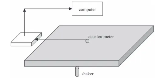
The experiment performed includes the introduction of load-induced damage in a reinforced concrete slab and the consequent vibration testing of the structure.

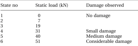
The experiment was performed in cycles. At each loading cycle, a static load is slowly applied at mid-span. Then the static load is removed and the slab is dynamically excited and its acceleration response is measured in the position indicated (Fig. 2). A random excitation signal is used for the dynamic experiment and the reason for this is that in most practical situations structures are subjected to ambi-ent excitation. Then a new increased static load is applied and the dynamic response of the slab is measured in its new state achieved after the removal of the load. The static load spanned from unloaded state to the ultimate state of failure. The experiment was performed and vibration data were taken for six loading levels. The applied static loads are given in Table 1. The dimensions of the slab are 14201420 mm2in plan and 75 mm in depth.

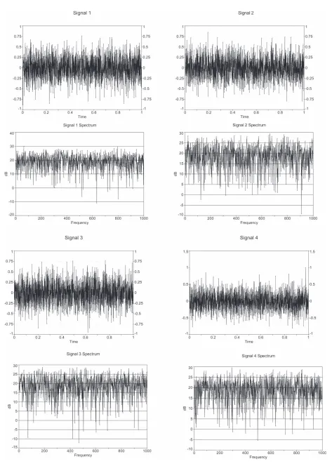
Figures 3(a) and 3(b) show the time signals and the corresponding spectra for four different cases includ-ing the non-damaged one. The measured accelera-tion signals are sampled at 0.0005 s. The signals were normalized against the maximum of the exci-tation signal. This figure shows random-like signals and broad-band spectra. A random response from a structure is not expected – some determinism should come from the structure itself. For a linearly behaving structure or one with behaviour close to linear, the resonant frequencies are expected to be detected. This is why non-linear behaviour is assumed, which might be explained by the non-linear material properties of the slab. Thus the methods of non-linear signal analysis are suggested to use for this case rather than concentrating on the structural modal characteristics. The determin-ism and the non-linearity of the signals are con-firmed subsequently, where some non-linear characteristics of these signals are estimated.

5.2 Recovering a proper state space

The first step towards using state space techniques is to establish proper characteristics for this state

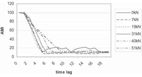
space, namely an appropriate time lag and a suffi-cient dimension. In this study, the AMI approach is used to find the proper time lag (see Section 2.1). A graph presenting the path of the AMI with the increase of the time lag is given in Fig. 4. The data for Fig. 4 were obtained according to equation (4) by forming the normalized histograms and the joint histogram of the measured signalss(n) ands(nþt). Figure 4 represents the AMI for the un-damaged case and for all the other levels of static pre-load (Table 1). It can be observed that the first minimum of the AMI changes with the introduction of damage: the smallest value of T is 5, which corresponds to 5 ms and it is obtained for the 0 pre-load case. The first minimum of the AMI for the next two cases of static pre-load can be observed at the same value of T, T¼5 ms. After the first three pre-loads, the

value of the first minimum of T increases, it goes up to 6 for the case of 31 kN pre-load and then jumps to 8 for the case of 40 kN pre-load. This tendency suggests that the degree of randomness (unpredictability) decreases with the introduction of damage and the signals become more ‘ordered’ and more ‘predictable’. A similar phenomenon has been observed for other test cases [5–8] and by other authors as well [3, 4]. Thus the time lagT, for which the first minimum of the AMI can be found, appears to be the first distinguishable feature which can be used for damage detection. In this study, it has already changed for the case of 31 kN pre-load (which can be considered as the first damaged state for the RC slab) and it keeps changing when damage grows. It is easy to estimate it from the graph for the AMI. The behaviour of the related damage feature FT as a function of the damage state is shown in Fig. 5.

5.3 Non-linear dynamic invariants for damage

detection

5.3.1 The average mutual information

As was previously explained, the AMI is a quantity which is easy and straightforward to compute directly from the measured acceleration series. The necessary operations are done easily and quite quickly on a PC and they result in the curves for

I(T_{) given in Fig. 4. The AMI forT}

¼2 ms is taken

to form the damage feature FI (see equation (6)),

but any other value of T which is smaller than the estimated time lag T0 can be used. Figure 5 gives the change of the suggested damage indexFIbased on the AMI with the change of the damage state.FI

remains 0 or close to 0 for the states after the first three pre-loads and then goes up to 41 per cent in the fourth stage (pre-load¼31 kN). This is the first

state when the slab can be considered damaged – in the previous three states, the slab remains practically undamaged. The index keeps increasing for the following damaged states of the slab.

5.3.2 The correlation dimension

In this particular case, the use of the correlation dimension proved to be impractical. The first obstacle was the estimation of proper global dimen-sion. Then the behaviour of the correlation function did not appear partially linear and it was difficult to find the mid-area and estimate its slope. Thus it ended up with a rather uncertain estimate for D2. For this reason, the results for the index FD (see equation (9)) should not be considered very reliable. These results are presented in Fig. 5. In this case, the index remains relatively close to 0 for the first three (practically undamaged) levels. It then increases for state 4, but then seems to drop somewhat for the following state and goes up again for the last state. In any case, either because the correlation dimen-sion was not reliably estimated or because of its irregular behaviour with damage, the index FD in this case does not seem to give information about the damage state of the slab.

5.3.3 The maximum LE

This is one of the cases when the maximum LE proves to be insensitive to damage. The LE itself shows a rather weak trend to decrease, but in general it stays very much on the same level between 0.18 and20.21. The relative change (the feature Fl, see Fig. 5) does not exceed 16.6 per cent, which is quite a small change compared with most of the other fea-tures. Moreover, the behaviour of the maximum LE and the corresponding feature Fl seems somewhat irregular:Fl increases to 16.6 per cent for the state after the 31 kN pre-load and it goes down to 11 per cent for the next damage state after the 40 kN pre-load.

5.4 Applying the statistics of the attractor for damage detection

The analysis of the data distribution on the attractor and its statistics proved much easier to carry out and Table 1 Static pre-loads and corresponding slab states

State no Static load (kN) Damage observed

1 0 No damage

2 7

3 19

4 31 Small damage

5 40 Medium damage

more useful for damage detection and quantification purposes.

5.4.1 Variance and skewness

Both characteristics showed a decrease with the introduction and the increase of damage. This is a trend, which should be expected: the decrease of the variance shows a decrease in the randomness of the points and the decrease in the skewness implies that the distribution approaches Gaussian. Some of the previously introduced dynamic charac-teristics already demonstrated a behaviour, which implies that the motion becomes more regular with the introduction and the extent of damage. The rela-tive changes of both statistics are shown in Fig. 5. It can be observed that both indexesFsandFgincrease for the state after the 31 kN pre-load and then they continue to increase for the next two states after the application of 40 and 51 kN.

5.4.2 The probability distribution

The average relative change in the coefficients cjy

given by equation (14) proves quite useful for damage detection purposes. The behaviour of Fc

with the damage state is also shown in Fig. 5. Fc

does not change and stays close to 0 for the first three states that correspond to the practically unda-maged slab, then it jumps to 40 per cent for the first damaged state after the 31 kN pre-load and keeps increasing with the increase of damage for the next two pre-loads going up to 84 per cent for the 51 kN state.

6 SOME COMMENTS AND CONCLUSIONS

This paper considers the possibility for using non-linear time series based dynamic characteristics for the purposes of damage detection and quantifi-cation. There are several reasons for exploring this approach.

1. The idea of using modal characteristics and modal description is that the system can be represented as a superposition of independent periodic oscil-lators. A lot of structures demonstrate non-linear dynamic behaviour due to non-linearities in their materials, joints, boundary conditions, etc. For such structures, the idea of modal analysis loses its importance and is not applicable when non-linearities become important. Then the tra-ditional way of analysing the dynamics of the structure and detecting damage in it using its modal contents cannot be applied. The analysis of the structural response using general time series analysis provides a more generic approach, which can be applied in such cases.

2. Using the traditional way of modal description of a vibrating structure for the purposes of damage detection has other disadvantages as well. The natural frequencies of many structures, especially the lower ones, do not show sensitivity to damage and cannot be used for damage detection. Frequently, the mode shapes turn out to be more sensitive to damage, but mode shapes are difficult to measure and characterize from experimental data and this makes them unsuitable for damage detection and characterization. In numerous practical cases even for structures with periodic and quasiperiodic behaviour, it might be difficult or even impossible to use modal characteristics for damage diagnosis purposes. The use of the measured time domain response of the structure is a more general approach and might well present a better alternative.

3. Vibration-based damage diagnosis assumes that changes in the dynamic characteristics of the structure are solely due to damage. In reality, a number of other factors such as changes in temp-erature and the environmental and operational conditions, noise can affect the dynamic behaviour of structures. The time series-based approach

Fig. 4 Average mutual information as a function of the

time lagT _{Fig. 5 The relative changes in per cent for the different}

is based on the long-term behaviour of the struc-ture and tries to extract the determinism from the signals. This is why it is expected to be more robust to the above factors. In fact there is evidence that for some applications, the time series-based characteristics are not significantly affected by noise and environmental changes [1, 4, 5, 13, 14].

This paper considers two possible time series-based approaches to dynamically characterize a vibrating system that present therefore two alterna-tive approaches towards vibration-based health monitoring – one based on the non-linear dynamic invariants and the other on the statistical analysis of the measured time series.

Most of the suggested damage features are applied on a test case of a reinforced concrete plate. Figure 5 represents a summary of the results and gives all the relative changes in per cent of the characteristics considered as possible damage features. The dashed lines correspond to changes in the non-linear dynamics invariants-based features – the proper time lag, the AMI, the maximum LE, and the correlation dimension. The solid lines represent the statistical features: the relative changes of the variance and the skewness and the average change in the p.d. function. Five of the represented features can be considered as appropriate for damage detec-tion and quantificadetec-tion. They are based on the time lag, the AMI, the variance, the skewness, and the probability distribution of the points on the attractor. These features show a considerable increase for the first state (after the 31 kN pre-load) and they retain their tendency to increase for the next two damage levels. Two of the features can be rejected as inap-propriate for detecting and characterizing damage for this case study, these are based on the maximum LE and the correlation dimension. These features show irregular behaviour as functions of the damage state (Fig. 5). The maximum LE demon-strates very low relative change in general, which does not increase with damage. The correlation dimension is somewhat more sensitive but it does not seem to show specific dependence on damage. The other consideration is the difficulty in estimating these characteristics. Their estimation cannot be considered robust and involves substantial compu-tation. In contrast, the other five characteristics, which have been concluded to be appropriate for damage diagnosis, are relatively easy and straightfor-ward to estimate from data, and they do show depen-dence on damage and on the extent of damage. The features based on the variance, the p.d., and the skewness show the highest sensitivity to damage and regular behaviour as functions of damage. The variance- and skewness-based features are the easiest of the three to estimate from data

once the proper time lagT0is found. The time lag in this case also shows regular increase with the extent of damage. Its change is minor when compared with the other features for the first damage state but its rela-tive change goes up to 100 per cent for the last damage state.

It should be mentioned that the damage sensitive quantities studied here can be estimated for any other structure provided its measured vibration response. Unfortunately, most of the parameters studied here, as well as those considered by other authors [3, 4], are very much case dependent. Factors influencing their estimation and behaviour include, but are not limited to, the type of structure, the material(s), and the type of damage. Therefore, draw-ing any general conclusions has been refrained so far because the relations have only been established for this test case and a couple of others. However, the general considerations to take into account when exploring time series structural response for the purposes of damage detection are as follows. 1. The non-linear dynamic invariants are in general

rather difficult to estimate from data.

2. In many cases they were found somewhat insensi-tive to damage.

3. The statistics-based characteristics are much easier and straightforward to estimate from data. 4. Statistical characteristics of the state space rep-resented response signals have been found damage sensitive for a number of test cases. 5. The statistics-based features should be preferred

to the non-linear dynamics invariants.

6. The time lagT0needed for reconstructing a state space is a characteristics which is rather easy to estimate from data. Also it is needed for the esti-mation of all the other characteristics suggested here. It should be considered among the first candidates for damage detection purposes if it has been established to show dependence on damage in a particular case.

ACKNOWLEDGEMENTS

The author acknowledges the support of NATO grant CBP.EAP,CLG.981517 for performing this research and for the preparation of the paper.

REFERENCES

1 Abarbanel, H.Analysis of observed chaotic data, 1996 (Springer-Verlag, New York).

3 Mathew, J.Some recent advances in signal processing for vibration monitoring. In Proceedings of the Fifth International Congress Sound and Vibration Adelaide, South Australia, 1997, pp. 903 – 918.

4 Todd, M., Nichols, J. M., Pecora, L. M.,andVirgin, L.

Vibration-based damage assessment utilizing state space geometry changes: local attractor variance ratio.

Smart Mater. Struct., 2001,10, 1000 – 1008.

5 Trendafilova, I. Vibration-based damage assessment using state-space representation of the structural response.Structural health monitoring 2002, Proceed-ings of the First European Workshop, Paris, July 2002, pp. 187 – 194.

6 Trendafilova, I.Nonlinear dynamics characteristics for damage detection. Proceedings of the III International Conference on Identification in engineering systems, Swansea, April 2002, pp. 155 – 164.

7 Trendafilova, I. State space modeling and represen-tation for vibration-based damage assessment. Pro-ceedings of DAMAS on Damage assessment in structures, 2003, pp. 547– 555.

8 Trendafilova, I.A state space based approach to health monitoring of vibrating structures. Modern practice in stress and vibration analysis, Materials science forum

(Ed. M. P. Cartmell), 2003, vol. 440 – 441, pp. 203 – 210 (Trans Tech Publications).

9 Krantz, H. and Schreiber, T. Nonlinear time series

analysis, 1997 (Cambridge University Press, Cambridge).

10 Fraser, A. M.andSwinney, H. L.Independent coordi-nates for strange attractors from mutual information.

Physica A, 1986,33, 1134 – 1140.

11 Craig, C., Nelson, R. D.,andPenman, J.The use of cor-relation dimension in condition monitoring of systems with clearance.J. Sound Vibr., 2000,231, 1 – 17.

12 Doebling, S. W., Farrar, C. R.,andPrime, M. B.A sum-mary review of vibration-based identification methods.

Shock Vibr. Digest, 1998,205(5), 631 –545.

13 Brincker, R., Anderson, P., Martinez, M. E.,andTavalo, F. Modal analysis of an offshore platform using two different ARMA approaches. Proceedings of the 14th Interantional Conference onModal analysis, 1994.

14 Hunter, G., Farrar, C., and Deen, R. Identifying damage sensitive features using nonlinear time series and bispectral analysis. Proceedings of the IMAC XVIII: Conference on Strucutral dynamics, 2000, 1796 – 802.

15 Pecora, L. M. and Carroll, T. L. Discontinuous and nondifferentiable functions and dimension increase induced by filtering chaotic data. Chaos, 1996, 6(3), 432 – 439.

16 Johnson, R. A. and Wichern, D. W. Applied

multi-variate statistical analysis, 2002 (Pearson Education

International, Germany GmBH).

APPENDIX

Notation

cjy coefficients of the probability densityp C(q,r) correlation function

D2 correlation dimension

D2un correlation dimension for the undamaged case

F vector function characterizing the dynamics of the system in its initial coordinate system

Fc damage index based on the coefficients

cjy

FD damage index based on the correlation dimension

Fg skewness-based damage index

FI damage index based on the average mutual information

Fl damage index based on the Lyapunov exponent

FT time lag-based damage index

Fs variance-based damage index

G(y(t)) mapping relation relatingy(tþT) and

y(t)

I(t) average mutual information

Iun average mutual information for the undamaged case

m the dimension of the state spacey p(Y) probability density of the attractor

^

p(Y) probability density of the attractor

P(s(n)) probability distribution ofs(n)

P(s(n),

s(nþt))

joint probability distribution ofs(n) and

s(nþt)

s(n) measured scalar variable

t time

T time lag

T0 time lag used for the reconstruction of the state spacey

Tun0 the time lag corresponding to the undamaged state

u(k) measured excitation values

w(k) measured response values

x defines the initial (but unknown) coordinate system of the dynamic system

y defines the new state space of the dynamic system

yNN nearest neighbour ofy

Yn set of vectors characterizing the attractor of the response

g_y skewness of attractor

g_yun skewness of attractor for the undamaged case

l1 maximum Lyapunov exponent

l1un maximum Lyapunov exponent for the undamaged state

fwj (y)g, j¼1,

2,. . ._,l

set of normalized Hermit polynomials

sy2 variance of attractor