Short-term prediction of traffic flow using a binary neural network

This is a repository copy of

Short-term prediction of traffic flow using a binary neural

network

.

White Rose Research Online URL for this paper:

http://eprints.whiterose.ac.uk/89459/

Version: Accepted Version

Article:

Hodge, Victoria J. orcid.org/0000-0002-2469-0224, Krishnan, Rajesh, Austin, Jim

orcid.org/0000-0001-5762-8614 et al. (2 more authors) (2014) Short-term prediction of

traffic flow using a binary neural network. Neural computing & applications. 1639–1655.

ISSN 0941-0643

https://doi.org/10.1007/s00521-014-1646-5

[email protected] https://eprints.whiterose.ac.uk/ Reuse

Items deposited in White Rose Research Online are protected by copyright, with all rights reserved unless indicated otherwise. They may be downloaded and/or printed for private study, or other acts as permitted by national copyright laws. The publisher or other rights holders may allow further reproduction and re-use of the full text version. This is indicated by the licence information on the White Rose Research Online record for the item.

Takedown

If you consider content in White Rose Research Online to be in breach of UK law, please notify us by

Short-Term Prediction of Traffic Flow Using a Binary

Neural Network

Victoria J. Hodgea, Rajesh Krishnanb, Jim Austina, John Polakb, Tom Jacksona

a

Dept of Computer Science, University of York, York, UK b

Centre for Transport Studies, Imperial College London, London, UK

{[email protected], [email protected], [email protected], [email protected], [email protected]}

Abstract.

This paper introduces a binary neural network-based prediction algorithm incorporating both spatial and temporal characteristics into the prediction process. The algorithm is used to predict short-term traffic flow by combining information from multiple traffic sensors (spatial lag) and time-series prediction (temporal lag). It extends

previously developed Advanced Uncertain Reasoning Architecture (AURA) k-nearest neighbour (k-NN) techniques. Our task was to produce a fast and accurate traffic flow predictor. The AURA k-NN predictor is comparable to other machine learning techniques with respect to recall accuracy but is able to train and predict rapidly. We incorporated consistency evaluations to determine if the AURA k-NN has an ideal algorithmic configuration or an ideal data configuration or whether the settings needed to be varied for each data set. The results agree with previous research in that settings must be bespoke for each data set. This configuration process requires rapid and scalable learning to allow the predictor to be setup for new data. The fast processing abilities of the AURA k-NN ensure this combinatorial optimisation will be computationally feasible for real-world applications. We intend to use the predictor to proactively manage traffic by predicting traffic volumes to anticipate traffic network problems.

Keywords- binary neural network; associative memory; k-nearest neighbour; time series;

spatio-temporal; prediction

Nomenclature

Variable = one feature of a traffic data vector, for example the flow value from a sensor.

Attribute = one time slice of one variable, for example the flow value from a sensor five minutes ago.

1 Introduction

Intelligent Decision Support (IDS) systems are an important computerised tool in many

problem domains. It is essential that any decision support system provides “intelligence”

to help with good decision making. IDS systems are used to analyse information,

establish models and support the decision making process. An IDS is predicated on

providing a supportive role rather than entirely replacing humans in the decision-making

process [1]. IDS has developed incorporating aspects from a broad spectrum of domains

such as: expert systems; artificial intelligence; database technologies and, data mining

and knowledge discovery.

The aim of our work is to provide an IDS tool to assist traffic network operators

to optimally manage traffic as a part of the FREEFLOW project [2]. This tool aims to use

neural-network-based pattern matching techniques to provide short-term predictions of

traffic volumes to the traffic operators and thus help them to select the most appropriate

course of action. The proposed IDS tool needs to operate in near “real time” and

dynamically; providing predictions prior to the next data collection, where traffic data are

updated every 5-15 minutes. Traffic monitoring and control systems produce large

volumes of data which infers that traditional relational databases are not suitable for

online traffic applications such as the IDS. Also, traffic data distributions are frequently

non-stationary; hence, any method needs to be able to accommodate non-stationary data

while still maintaining fast, flexible processing. The proposed methodology could be

extended to other monitoring applications that use spatially distributed sensors where

neighbourhoods of sensors exist and where temporal characteristics are important.

In the remainder of this paper, we provide a concise review of traffic flow and

neural network-based prediction methods in section 2, section 3 discusses our proposed

binary neural network predictor, sections 4 provides an evaluation of our proposed

prediction method against alternative machine learning methods. The evaluation analyses

the prediction accuracy; and examines whether there is a single algorithm configuration

and whether there is a single data configuration that performs best with respect to

prediction accuracy. The evaluation is focused on the timing analyses of the training and

the execution time of our proposed technique. We then analyse the results of the

evaluations in section 5 and provide our conclusions in section 6.

2 Short-term Prediction

The focus of our work in this paper was to predict future traffic flows over short-term

traffic operator to allow them to visualise how the traffic will develop over the near future

and to anticipate traffic problems. We provide a selective review of time series prediction

literature with particular reference to vehicle flow prediction and neural network-based

predictors.

Well-known short-term prediction algorithms can broadly be classified into

univariate and multivariate approaches. Simple univariate prediction models predict the

value of a variable as a function of the same variable observed in the immediate past.

Ding et al. [4] used support vector machines [5] to model future traffic flows at a given

location as a function of past flow observations at the same location. The ARIMA

methodology introduced by Box and Jenkins [6] is a popular statistical approach for time

series prediction. Hamed and Al-Masaeid [7] used an ARIMA time-series model to

predict 1-minute future traffic flows. Williams et al. [8] added seasonal differencing to

the ARIMA model to predict 15-minute-ahead flows with a periodicity of 24-hours. More

recently, Ghosh et al. [9] used a seasonal ARIMA model calibrated using Bayesian

methods to predict traffic flows. However, the ARIMA method requires time consuming

manual configuration for each problem scenario to obtain accurate prediction results. In

addition, it is not easy to incorporate additional explanatory variables other than the

observed variable in the ARIMA framework.

In contrast, a multivariate approach uses data from several locations for traffic

prediction. The traffic flow on a road network is a spatial-temporal process. The traffic

variables observed at a given location are correlated with the present and past values of

the same traffic variables observed at upstream or downstream locations. Hence, traffic

prediction models often use observations from neighbouring sensor locations as

explanatory variables to predict the value of a sensor variable at a given location.

Neural networks are often used for traffic variable prediction but many neural

networks require intensive tuning to ensure optimal performance. Amin et al. [10] used a

Radial Basis Function (RBF) neural network to perform traffic flow prediction. In an IDS

application, the neural network would need to be retrained every time new data became

available which is likely to be daily. It is also likely that different parameter sets would be

required for different locations on the road network. This training and retraining

introduces high computational complexity. For example, Vlahogianni et al., [11]

demonstrated a genetic algorithm for optimising Multi-Layer Perceptrons (MLPs) with

respect to the learning settings and the hidden layer topology. The optimised neural

network was then used for short-term traffic flow prediction. Abdulhai et al. [12]

demonstrated a similar approach for traffic flow prediction by using genetic algorithms to

multiple links between neurons. These additional links introduced a time delay between

network layers to capture the evolution of vehicle flow over time.

Martinetz et al. [13] used the neural gas network for chaotic time series

prediction. Neural gas extends both k-means clustering and Kohonen neural networks.

Predictions are generated from learning input to output mappings where the output is the

future value associated with the training example (input value). Zhang et al. [14]

developed a Bayesian network model to describe the traffic flows. Their approach used a

Gaussian Mixture Model to approximate the joint probability distribution within the

Bayesian network nodes following dimensionality reduction by Principal Component

Analysis.

Kindzerske and Ni [15] are one of a number of authors to realise Yakowitz’s [16]

developmental work by applying non-parametric regression, the k-NN algorithm, to time

series prediction. Kindzerske and Ni [15] represented the current snapshot of the traffic

sensors as a vector and compared this vector against historical vectors. The best matching

historical vectors are then combined to generate a prediction. Krishnan and Polak [17]

enhanced this by introducing temporal lag in their k-NN approach so that each of the

sensor’s variables formed a time series and the set of all time-series were concatenated to

produce a vector covering the spatial distribution of sensors.

In a similar manner, Kamarianakis and Prastacos [18] introduced a spatio-temporal

extension of ARIMA to predict future flows as a function of historical flows from a given

location and its upstream locations.

The accuracy of prediction depends on both the appropriateness of the data

configuration and the correct implementation of the machine learning tool. For

spatio-temporal data, simply incorporating spatially distributed sensors and attributes may

actually generate predictions that are worse than non-spatial models unless the data from

these neighbouring locations influence the predicted value. Kamarianakis and Prastacos

[18] showed that injudicious use of data from neighbouring locations may actually

decrease prediction accuracy. They showed that using relatively few, dispersed sensors

fails to account for the spatial dependencies. Conversely, they found that as the number of

sensors increases, the prediction accuracy may improve significantly if spatio-temporal

relationships are captured.

To summarise, traffic prediction models need to (1) accurately model historical

traffic flow patterns, (2) account for both the intra-day and inter-day variability in traffic

variables, (3) be able to incorporate both temporally and spatially distributed information,

where appropriate, to improve prediction accuracy and (4) generate predictions rapidly

2.1

Our approach

In this paper, we develop a fast and scalable neural network-based k-NN predictor

implemented using the AURA binary neural architecture. It is adapted from the

methodology described in [17] which incorporated temporal and spatial lag into standard

k-NN traffic flow prediction.



processing. Traffic data change over time which necessitates a temporal

component for prediction.



allow future traffic flows to be estimated.

The resultant method predicted future traffic flows by matching a current time

series pattern against historical data patterns and using these matching time series to

predict either how the current traffic state will develop over time or what may happen if a

particular control mechanism is implemented. The methodology described is fast, flexible

and satisfies the four criteria above. It also has wider application to other time series

prediction tasks, beyond the prediction problem addressed in this paper, for example,

[19], [20].

3 Binary Neural Network for prediction

The objective for the neural network-based pattern matching method was to predict the

future traffic flows to allow the traffic operator to visualise how the traffic situation will

develop. The AURA k-NN method identified a set of historical time periods when the set

of traffic observations on the road network were most similar to the current observations.

It then used this information to produce a prediction of the future traffic flow by

averaging the flow development across the set of matches.

3.1

AURA k-NN

K-NN is a nonparametric pattern matching technique known to be robust and flexible

and allows the predictor to be updated continuously. However, a drawback of

conventional k-NN is its speed, as it becomes very slow for large problems. This

drawback is overcome by using the AURA neural network technique to underpin the

k-NN. Using AURA means that the AURA k-NN can perform up to four times faster than

the standard k-NN [21]. AURA is a group of techniques designed for high speed search

Matrix Memory (CMM): a binary matrix used to store and retrieve patterns [22]. In the

AURA k-NN developed previously [21, 23, 24, 25], each column of the CMM was a set

of attribute observations for a record (pattern) and each row indexed an attribute value or

a quantised range of values. AURA applies input patterns to the CMM to act as a cue to

retrieve similar output patterns. We extended the approach to match time-series vectors

and then to generate short-term predictions in this paper. The details of the AURA k-NN

implementation are given in the following text.

3.1.1 Time Series

In the traffic domain, the AURA k-NN can process a broad spectrum of traffic variables

such as vehicle counts, vehicle speeds, bus timetable adherence, traffic signal settings,

congestion metrics, roadworks data, events data, and weather data. In this paper, we used

flow and occupancy data from sensors located in the roads. Flow is the number of

vehicles passing over the sensor during unit time and occupancy is the percentage of time

vehicles are present over the sensor during a specific time period.

For traffic prediction, the system must incorporate time: traffic data are dynamic

and show recurring patterns with respect to time. We describe how we accommodated

temporal aspects into the pattern match.

Given the current set of observations,Xn, from the set of traffic sensors and a

dataset of historical records {X}, k-NN identifies theknearest neighbours ofXnin {X}

using a distance metric. In this paper, the data records were time-series representations of

spatially distributed sensors to incorporate trend similarity and spatial awareness into the

prediction approach. To produce the time series, the AURA k-NN effectively buffered

historical data and accumulated data for a preset time interval,PT. It always preserved the

temporal ordering of the data, thus,Bufferv= {Buffervt:t PT} represents the time series

buffer of variablevof the data. The time-series for recordXnwhich we callXn

TS

becomes

equation 1:

X

= {x

, x

, x

, x

, x

, x

,…,x

, x

, x

, x

}

(1)

forPTof four time lags {t-3, t-2, t-1, t}. The results of our evaluations in section 4 show

that the number of time lags needs to be tuned for each data set.

For example, for two sensors reporting two variables: flow and occupancy, where

sensor1has readings of 51, 62, 55, 68 for flow and readings of 15.0, 18.0, 21.0, 29.0 for

occupancy for four time lags {t-3, t-2, t-1, t} respectively and sensor2has flow readings

of 38, 38, 56, 58 and occupancy readings of 15.0, 16.0, 23.0, 25.0 respectively, thenXn

TS

is given in equation 2:

Xn

TS

where the vertical bars illustrate the sections of the pattern with each section representing

the time series buffer for one sensor variable (flow or occupancy here).

3.1.2 Learning

The CMM is used in AURA to store representations of all data. The CMM is anm × n

binary matrix that learns theNrecords in the data set. During learning, the CMM forms

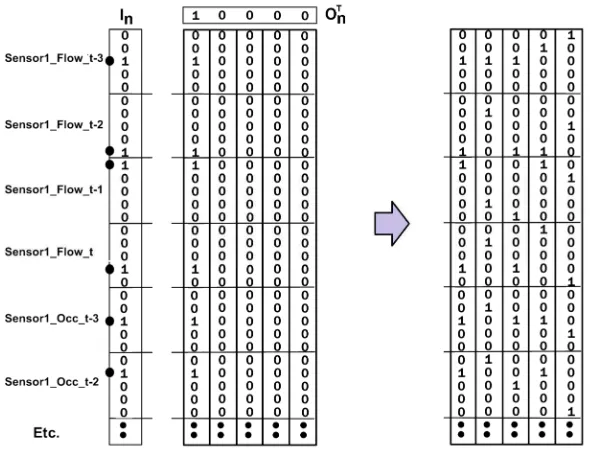
an association between an input pattern and an output patternIn Onfor each recordn

whereInandOn {0,1} as shown in figure 1.

Figure 1. Showing the CMM storing the first associationI0×O0on the left and a CMM trained with five associations on the right.

The input pattern (In) represents the concatenated set of all time-series buffer

values for all variables of a particular recordXn

TS

and indexes matrix rows. In the

remainder of this paper, each value of each time series buffer of each variable is referred

to as an attribute. There are 16 attributes in equation 2. The associated output vector (On)

uniquely identifies that record and indexes the matrix columns. Thus, the set of attribute

values for recordnare associated with a unique identifier for the record. In figure 1,I0is

stored in the leftmost column of the CMM and is uniquely indexed byO0(10000) which

activates the leftmost column.

The CMMs require binary input patterns for computational efficiency while

training and matching; so numeric attributes must be quantised (binned) to allow mapping

to a binary pattern [21]. Quantisation maps a continuous-valued attribute into a smaller

("finite") set of discrete symbols or integer values. Each attribute is quantised over its full

range of values and mapped to a set of bins. This allows each bin to index a specific and

unique row in the CMM. For example, for an integer-valued attribute with range 0-99 and

For a real-valued attribute with range [0.0-100.0] and five bins then each bin would have

width 20:bin0[0.0, 20.0),bin1[20.0, 40.0) …bin4[80.0, 100.0]. Thus, for the sensor1and

sensor2above, the set of bin mappings forXn

TS

in equation 2 are given in equation 3:

Bins

(

X

) = {2, 3, 2, 3, | 0, 0, 1, 1, | 1, 1, 2, 4, | 0, 0, 1, 1}

(3)

In the AURA k-NN, each bin index maps to a binary representation to generate

the binary patterns for AURA. For an attribute with five bins, the five possible binary

representations are:bin0= 00001,bin1= 00010,bin2= 00100 etc. To produce the input

vectorInto train into the CMM, the binary representations for all the attributes in the data

pattern are concatenated. The bin indexes for all attributes inXn

TS

are set to 1 while all

other bin indexes remain unset (0). The binary input vectorInderived from the bin

mappings in equation 3 is given in equation 4. This is the input learning pattern to be

stored in the CMM to allow the particular associationIn×Onto be stored and retrieved

I

= {00100 01000 00100 01000 | 00001 00001 00010 00010 | 00001 … } (4)

Each binary input patternInis associated with a unique binary output patternOn

which has a single bit set to index a single column in the CMM. This column thus

uniquely indexes the binary patternIn. For example,O0(10000) uniquely indexesI0

which is the leftmost column in figure 1.

The CMM stores an association for allNrecords in the data set {XTS}. Thus, the

CMM represents {(I1×O1), (I2×O2), … (In×On)}. Learning is a one-pass process with one

learning step for each record in the data set. Hence, training is rapid. CMM learning is

given in equation 5.

T n n N

n

O I

CMM 

1



where

is logical OR

(5)

T n n O

I  _{is an estimation of the weight matrixW(n) of the neural network as a linear}

associator.W(n) forms a mapping representing the association described by thenth

input/output pair. The CMM is then effectively an encoding of theNweight matricesW.

Individual weights within the weight matrix update using a generalisation of Hebbian

learning [26] where the state for each synapse (matrix element) is binary valued. Every

synapse (matrix element) can update its weight independently and in parallel.

EachInhasmbits set wheremis the number of attributes (assuming no missing

values) and eachInis of lengthm•bwherebis the number of bins per attribute. Each On

has 1 bit set and has lengthN. There areNassociations (one per data record). Therefore,

the CMM containsm × Nset bits, i.e., mbN b mN 1 

possible bits are set in the CMM after

each output pattern and the CMM are represented by the indices of the set bits only. This

means that only b 1

indices need to be stored for the CMM. This is similar to the pointer

representation used in associative memories [28]. This compact representation ensures

that retrieval, as described next, is proportional to the number of set bits in both the

retrieval pattern and the CMM and is fast and scalable.

3.1.3 Retrieving the best matches

During retrieval, the CMM is searched to find thekbest matches. Each query record is of

the same format as the records in the training data (see equation 2). For each new query

Xq

TS

, a retrieval patternRis created.Ris formed from a set of parabolic kernels, with one

kernel for each attribute inXq

TS

. The kernels emulate Euclidean distance [21] to allow us

to emulate standard (Euclidean) k-NN. For each time slice for a particular variable, the

kernels are identical but they may vary across variables according to the number of bins

assigned to that variable. For example, a flow variable may use a different number of bins

compared to an occupancy variable. In this paper, all attributes use an equal number of

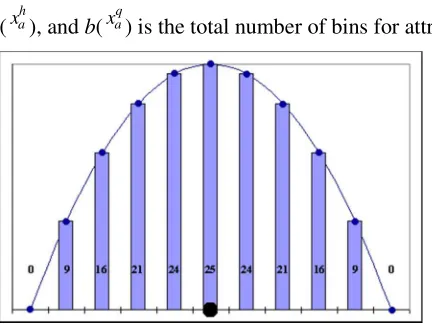
quantisation bins and, hence, an equivalent kernel. The kernel density is estimated using

equation 6 for all attributesainXq

TS

and an example kernel is shown in figure 2.









(6)

Where,max(b) is the maximum number of bins across all attributes, |bin(

q a

x _{) –bin(}x_ah_{)| is}

the number of bins separating the bin mapped to by this attribute value for the query

pattern (

q a

x _{) from the bin mapped to by this attribute value for the stored historical pattern}

(

h a

x _{), andb(}xaq_{) is the total number of bins for attributex} a.

Figure 2. Showing the kernel values produced from equation 6 to approximate Euclidean Distance. To emulate the scoring of Euclidean Distance, the kernels for all attributes are

query record. This ensures that the query value itself receives the highest score and the

score reduces according to the distance from the query value. For an integer-valued

attribute with range 0-99 and five bins then each bin would have width 20:bin0{0..19},

bin1{20..39} …bin4{80..99}. Thus, if the query record value was 31 this would map to

bin1so the input vector element representing bin1would be the centre of the kernel. The

highest value for this kernel (analogous to the dotted value of the kernel in figure 2)

would be centred onbin1.

For Euclidean kernels, the retrieval pattern input to the CMM to retrieve the topk

matches is iteratively given by equation 7:

R´ = R



offset

(

Kernel

(

x

)), for all attributes

x

(7)

whereoffset() indexes attributexa’s section of the input patternRand ensures that the

kernel is added toR,centred on the query value for attributexaandis the concatenation

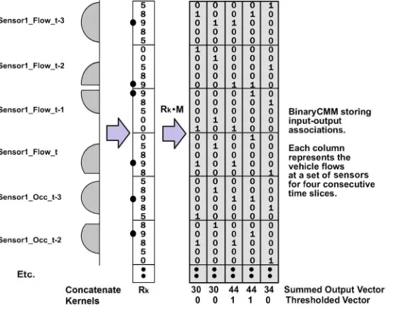
operator. Thus, each attribute indexes a defined set of elements inRas shown in figure 3.

Figure 3. Illustrating the application of kernels to a CMM to find the k-nearest neighbours using time-series vectors. The kernels are mapped onto an integer vectorRkwhich is applied to the

binary CMM by multiplying the CMM rows by the integer values. The CMM summed output vector is thresholded to retrieve thekbest matches.

WhenRis applied to the CMM to retrieve the best matches, the values inR,

multiply the rows of the matrix as shown in figure 3. If the bit is set to one in a particular

column, then the column will receive the kernel score for the corresponding row as given

in equations 7 and 8. The process is illustrated in figure 3. For Sensor1_Flow_t-3,

columns 1 and 2 (indexing from 0 on the left) receive a score of 9 as the set bit in the

respective columns aligns with the score of 9 in the input kernel. In contrast, the right

column receives a score of 5 as the set bit in the right column aligns with the score of 5 in

To retrieve the best matching records, the columns (one column per record) of the

matrix are summed according to the value on the rows indexed by the query input pattern

Rand the CMM produces a summed output vectorSas given in Equation 8.



 R CMM

ST

(8)

The summed output vector is then thresholded using L-Max thresholding [29] to

produce a binary thresholded vectorT. L-Max thresholding is used in the AURA k-NN as

it retrieves the topLmatches. After thresholding,Teffectively lists the topLmatching

columns which represent the topk(wherek=L)matches; i.e, theknearest neighbours.

This is also illustrated in figure 3.

The overall retrieval time is proportional to the number of set bits in both the

retrieval vector and the CMM. If the retrieval vector is a binary vector, similar toInused

in training, then retrieval from the CMM is a count of the number of exact matching

binned attribute values for every stored recordnN. If we assume that on average each stored vector (matrix column) matches 50% of the input and we assume the set bits are

equally distributed across the rows then only 2 mN

bits are examined during retrieval

wheremis the number of attributes. We performed recall accuracy investigations using a

number of different kernels for retrieval and using the Euclidean kernels significantly

improves recall accuracy compared to other approaches [30]. However, the accuracy

increase is at the expense of a slight speed decrease compared to using a single bit set

pattern. The Euclidean kernel excites all CMM rows of the attribute if the kernel is

centred on the middle bin and half of the rows if centred on one of the extreme value bins.

If we assume that on average 75% of the rows are excited for each attribute and the bits

are equally distributed across the rows then 4 3mbN

bits are examined during retrieval.

Thus, the kernel based AURA k-NN has runtime growth of 

   

4 3mbN

wheremb<<Nso

this is approximately equal to growth proportional to O(n) wherenis the number of

records.

3.1.4 Prediction

For the prediction task in this paper using data arriving at 15 minute intervals from the

sensors, we retrieved thektop matches and then looked up thet+1(+15 minute) ort+4

(+1 hour) sensor values for each of thekmatches (these are stored in a database). Thet+1

(+15 minute) prediction is then the mean value of the set oft+1values from theknearest

4 Evaluation

We evaluated our AURA k-NN prediction method against a number of predictors

implemented using WEKA 3.6 software [31]. WEKA [32] is a Java GUI-based

application that contains a set of machine learning algorithms designed for data mining.

The algorithms can be used for tasks including data pre-processing, classification,

prediction and clustering. Note WEKA prediction is to 3 decimal places whereas AURA

predicts to integers to display to the traffic operator. The methods used were;

1. Standard k-NN[33] known as Instance Based learning (IBk) in WEKA 3.6 - we

usedk=50 andk=10 in our analyses.

2. Multi-Layer Perceptron(MLP) Neural Networksare feedforward supervised

neural networks with at least one layer of nodes between the input nodes and output

nodes. The network links flow forward from the input to the output layer. The

network is trained by the backpropagation learning algorithm [34] using historical

data. Training creates a model that maps inputs to outputs and this model can then be

used to predict the output when new data is applied. MLPs have been used for traffic

prediction on a number of occasions. For optimum results, the parameters of the MLP

are intensively tuned; for example, using a genetic algorithm [11]. However, this

intensive tuning process is too slow for an on-line application such as the IDS.

Nevertheless, we ensured that we evaluated at least as many parameter sets for the

MLP as we evaluated for the AURA k-NN. For all evaluations, the MLP used

learning rate decay, train and validate (using 30% of the training data for validation)

and we varied the key MLP parameters: learning rate and momentum. All other

settings were WEKA defaults as these produced the best prediction accuracy. An

example WEKA MLP configuration is listed in the Appendix showing the settings

that we varied. Learning rate determines the amount the network weights are updated

as training proceeds. Decaying the learning rate “may help to stop the NN from

diverging from the target output as well as improve general performance”. Using a

train and validate regime ensures that the training data are split between actual

training data and validation data. Validation data are used to test the trained network

and stop training before performance degrades.

3. Support Vector Machine(SVM) is implemented as SMOreg in WEKA 3.6 and

implements the support vector machine for regression [31][35]. Support vector

machines map the data to a high dimensional feature space and generate linear

boundaries in the feature space to represent the non-linear class boundaries. SMOreg

implements sequential minimal optimisation to train the support vector regression and

all attributes are normalised. Again, we ensured that we evaluated at least as many

an RBF kernel and we varied the complexity. Labeeuw et al. [36] assessed various

machine learning techniques for the similar task of predicting traffic speeds and

congestion. They concluded that SVMs with an RBF kernel had the highest accuracy

of the methods evaluated so we used it here. All other settings were WEKA defaults

as these produced the best prediction accuracy. An example WEKA SVM

configuration is listed in the Appendix showing the settings that we varied.

4. Least Median Squares (LMS) regression– In WEKA, the LMS regression

functions are generated from random subsamples of the data. The LMS regression

with the lowest median squared error is then used as the final model. Our

implementation used all default settings.

The performances of the various configurations of the AURA k-NN were

compared against each other based on their prediction accuracy over an independent test

set (out-of-sample accuracy) using the metrics in equations 9, 10 and 11. The MLP, SVM

and LMS provided baseline accuracies to allow us to compare the standard k-NN and

AURA k-NN prediction accuracies using the metric in equation 11.

Mean Percentage Error (MPE) =

X F X n i i i i



(9)

- measures the bias (over-estimating or under-estimating)

Mean Absolute Percentage Error (MAPE) =

X F X n i i i i



(10)

- measures the goodness-of-fit

Root Mean Squared Error (RMSE) =







(11)

- Measures the absolute error – this is the best metric for comparing different methods.

4.1

Data

In our application the IDS is required to run in near real-time so we need to minimise the

data pre-processing. The only pre-processing performed was to clean the two data sets

used using a simple rule: Univariate Screening given in Krishnan [37]. If a historical

record contained an erroneous value then the entire record (one vector in the training set)

was removed.

For the WEKA algorithms evaluated, the training data comprised the data vector

value). For +15 minute prediction, the training vector was the vector from equation 2 with

thet+1sensor reading as the class value. Accordingly, for +1 hour prediction, the

training vector was the vector from equation 2 with thet+4sensor reading as the class

value. To generate the prediction, the algorithm predicted the class value from the query

data vector. The algorithms were tested using two traffic data sets from central London in

Russell Square and Marylebone Road.

4.1.1 Data Set 1

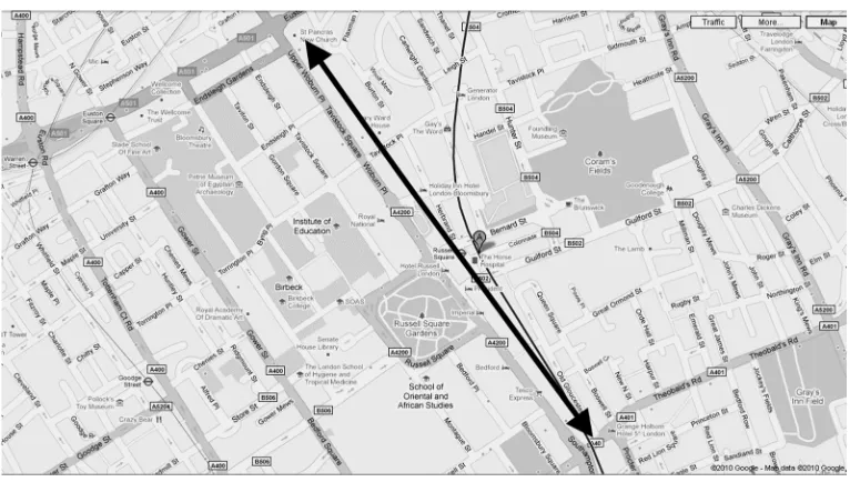
Figure 4. The Russell Square corridor in central London (Source: Google Maps).

Data from seven sensors arranged in series along the Russell Square corridor

(southbound) in central London (see figure 4) was the first data set used for the prediction

experiment in this paper. The flows on the southernmost (downstream) sensor were

predicted. All sensors output two attributes: 15-minute flow values (which vary between

0-800) and 15 minute occupancy values (with data range 0.0-100.0). The data were

obtained for the months of June, July and August 2007. Data from June and July were

used as the training set and data for August formed the test set. The training and test data

sets comprised only data from weekdays (Monday to Friday) with 3,840 training records

4.1.2 Data Set 2

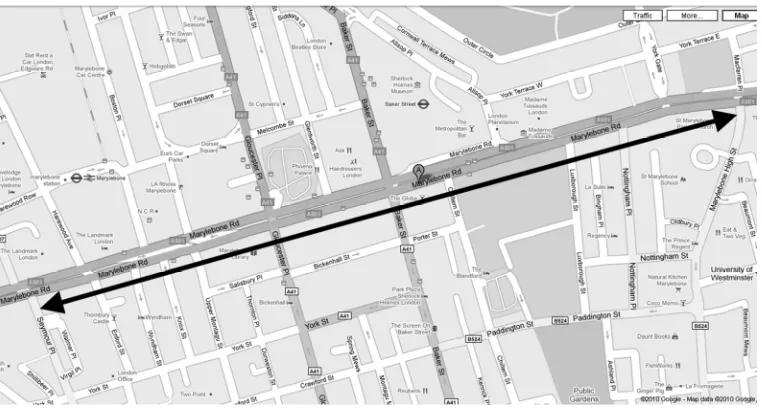
Figure 5. Marylebone Road in central London (Source: Google Maps).

Data set 2 comprised data from six sensors on Marylebone Road (eastbound) in

central London (see figure 5) where the future flow values at the easternmost

(downstream) sensor were predicted. The six sensors output 15-minute flow values with

data range 0-1600. Training data were from May 2008 and 1st-13th June 2008 while test

data were from 16th-20th June 2008 (one week). Only the weekday data were used giving

2,976 training records and 480 query records. A severe traffic incident happened in

Marylebone Rd on 20th June from 18:59 to 21:01. We ran two analyses, one using all of

the test data from 16th-20th June and a second analysing data from the 20th June, the day

the incident occurred which comprised 96 records. The latter analysis provided an

indication of how well the various machine learning techniques performed on incident

data when the traffic flow would be anomalous and prediction is potentially more useful

to end-users.

4.2

Tests

We ran seven separate tests to: find the best AURA k-NN parameter settings; pinpoint the

best data configurations; compare the accuracy of the predictors; and, ultimately, evaluate

the training and query time of the AURA k-NN. Parameter setting is a combinatorial

search problem and both algorithmic and data-related parameters may be varied. Hence,

we did not exhaustively test every possible parameter combination as this would be

computationally intractable. Instead, we analysed a range of data and algorithm settings

to evaluate both accuracy and consistency and whether we need to use bespoke settings

for each data set. Tests 1-3 use data set 1: the data for Russell Sq. in June, July and

August, 2007. Tests 4-7 use data set 2: the data for Marylebone Rd in May and June,

4.2.1 Test 1 – the best AURA k-NN configuration

This test was to investigate the best configuration with respect to the internal parameters

of the AURA k-NN. These parameters were: the length of the time series (TS); the number of bins (Bins); and, thekvalue for k-NN (k). We varied the setting of the parameters in turn and counted the number of times each setting had the lowest RMSE

across the evaluations of that parameter. The results are listed in table 1.

Table 1. Table with count of the number of times each AURA k-NN parameter setting has the lowest RMSE. The highest counts forTS,Binsandkare shown in bold.

TS Bins k

2 4 6 8 10 11 25 49 10 25 50 100

RMSE – 15 mins 0 0 0 4 3 1 0 7 0 0 11 0

RMSE – 60 mins 0 0 0 5 2 6 0 2 0 4 7 0

The most consistent time series length andk-value are clear (TS=8 andk=50,

respectively). The number of quantisation bins to use was less clear. When predicting +15

minutes, 49 quantisation bins performed best. When predicting +1 hour, 11 bins generally

performed best as this has the highest winning count. However, the two best performing

configurations for +1 hour with respect to both MAPE and RMSE use 49 bins rather than

11 bins.

Test 1 indicated that optimising the algorithm configuration was important and

needed care.

4.3

Test 2 – the best data configuration

Test 1 evaluated the AURA k-NN settings so test 2 evaluated different data

configurations to find the optimal data configuration(s) for prediction with AURA k-NN.

In test 2, we used the best AURA k-NN configuration from test 1 (TS=8,Bins=49,k=50)

and evaluated the following data settings: the number of sensors (NS)to use, whether to incorporate the attributes of the sensor,self, whose flow is being predicted (S) and

whether to incorporate the occupancy attribute (O). All evaluations used the flow attribute (F). Each configuration was given a label to allow it to be referenced in the text. The results of test 2 are given in table 2.

Table 2 shows that there was a clear difference between the best and worst RMSE

for both +15 minute and +1 hour prediction. Configurations 1-6 and 1-7 performed best

with respect to both RMSE and MAPE.

From table 2, configurations 1-6 and 1-7 have higher MPE than the other

configurations indicating that they overestimate more while the other configurations

alternate between under and over estimations of larger magnitudes. The occupancy

necessity as the other best performing configuration did not use occupancy. Including all

sensors produced higher accuracy compared to limiting the number of sensors. Including

the self-sensor improved accuracy with the flow attribute only but did not improve

accuracy with both flow and occupancy attributes. Again, this indicates that the data need

to be carefully configured.

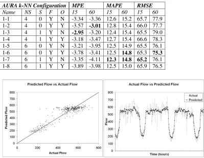
Table 2. Table listing the MPE, MAPE and RMSE for the various data configurations of the AURA k-NN. 15 indicates +15 minute ahead prediction and 60 indicates + 1 hour ahead prediction. The highest prediction accuracy for each column is shown in bold.

AURA k-NN Configuration MPE MAPE RMSE

Name NS S F O 15 60 15 60 15 60

1-1 4 0 Y N -3.34 -3.36 12.6 15.2 65.7 77.9 1-2 4 0 Y Y -3.57 -3.01 12.8 15.4 66.0 77.7 1-3 4 1 Y N -2.95 -3.20 12.4 15.4 65.5 79.0 1-4 4 1 Y Y -3.18 -3.47 12.7 15.4 66.6 78.3 1-5 6 0 Y N -3.21 -3.95 12.5 14.9 65.5 76.1 1-6 6 0 Y Y -3.78 -3.41 12.5 14.8 65.3 75.3

1-7 6 1 Y N -3.35 -4.11 12.3 14.8 65.2 76.1 1-8 6 1 Y Y -3.89 -3.98 12.5 15.0 65.9 76.5

Figure 6. Scatter plot and line graph for the actual and predicted flow values for +15 minute prediction (t+1) for AURA k-NN configuration 1-6.

The prediction results for configuration (1-6) are plotted in figures 6 and 7 against

the actual data values. The scatter plot and line graphs in figure 6 show the prediction

accuracy for +15 minute prediction and the graphs in figure 7 show the prediction

accuracy for +1 hour prediction. This illustrates where the prediction is accurate and

where it is inaccurate across the time span of the test data. From figures 6 and 7, the

AURA k-NN tends to smooth transient spikes, particularly transient spikes where the

flow values suddenly decrease supporting our earlier conclusion that configurations 1-6

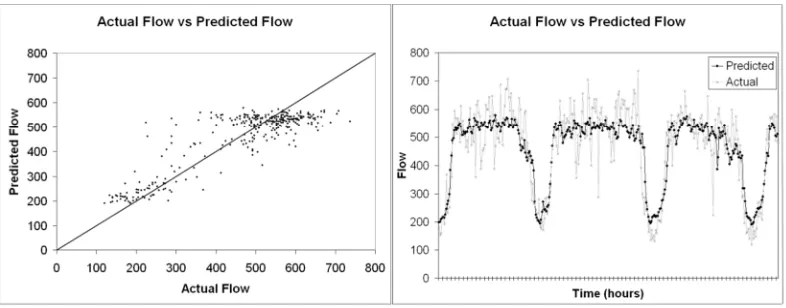
Figure 7. Scatter plot and line graph for the actual and predicted flow values for +1 hour prediction (t+4)for AURA k-NN configuration 1-6.

4.3.1 Test 3 – comparison to other algorithms

Next, we took the two best performing data configurations (1-6 and 1-7) from test 2 and

compared AURA k-NN to the WEKA machine learning algorithms running these two

data configurations.

 AURA k-NN and standard (WEKA) k-NN :k_=50.

 MLP config 1.6: learning rate = 0.4, decay = true, momentum = 0.3  MLP config 1.7: learning rate = 0.5, decay = true, momentum = 0.4.  SVM config 1.6: RBF Kernel, complexity = 50.0

 SVM config 1.6: RBF Kernel, complexity = 75.0.

The recall accuracy results for configuration (1-6) are listed in table 3 and the

results for (1-7) are listed in table 4.

Table 3. Table comparing the recall accuracy of the various predictors with time series length 8, flow and occupancy attributes and predicted sensor excluded (six sensors) for test 4 part 1. The highest prediction accuracy for each row is shown in bold.

AURA k-NN_ 1-6 k-NN MLP SVM LMS

RMSE – 15 mins 65.3 65.3 68.1 69.4 69.9 RMSE – 60 mins 75.3 75.3 80.5 80.5 85.7

For configuration 1-6, the AURA k-NN and the standard k-NN were the joint

best performing predictors for both +15 minute and +1 hour prediction compared to the

other approaches.

Table 4. Table comparing the recall accuracy of the various predictors with time series length 8, flow attribute only and all sensors for test 4 part 2. The highest prediction accuracy for each row is shown in bold.

AURA k-NN_ 1-7 k-NN MLP SVM LMS

The AURA k-NN was the best performing for both +15 minute and +1 hour

prediction for configuration 1-7, closely followed by the standard k-NN. The RMSE

varied for all algorithms between this data configuration and the previous indicating that

all algorithms need to optimise the data configuration

4.3.2 Test 4 – the best data and AURA k-NN configuration

The first test of the AURA k-NN for data set 2 was to evaluate different configurations to

find the optimal configuration(s) for prediction. For Marylebone Rd, we ran a single

algorithm/data configuration test as only flow data was available whereas Russell Sq. had

both flow and occupancy. The results are given in table 5. We evaluated: whether to

incorporate the attributes of the sensor whose flow is being predicted (S); the time series length (TS); the number of bins to use for quantisation (Bins); and, thekvalue for AURA k-NN (k).

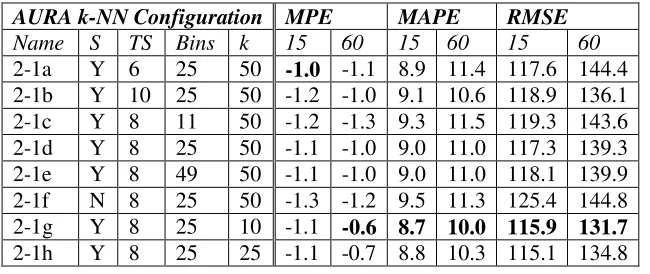
Table 5. Table listing the MPE, MAPE and RMSE for various configurations of the AURA k-NN with time series length 8 using the full week of query data. 15 indicates +15 minute ahead prediction and 60 indicates + 1 hour ahead prediction. The highest prediction accuracy for each column is shown in bold.

AURA k-NN Configuration MPE MAPE RMSE

Name S TS Bins k 15 60 15 60 15 60

2-1a Y 6 25 50 -1.0 -1.1 8.9 11.4 117.6 144.4 2-1b Y 10 25 50 -1.2 -1.0 9.1 10.6 118.9 136.1 2-1c Y 8 11 50 -1.2 -1.3 9.3 11.5 119.3 143.6 2-1d Y 8 25 50 -1.1 -1.0 9.0 11.0 117.3 139.3 2-1e Y 8 49 50 -1.1 -1.0 9.0 11.0 118.1 139.9 2-1f N 8 25 50 -1.3 -1.2 9.5 11.3 125.4 144.8 2-1g Y 8 25 10 -1.1 -0.6 8.7 10.0 115.9 131.7

2-1h Y 8 25 25 -1.1 -0.7 8.8 10.3 115.1 134.8

Again, there is a clear difference between the best RMSE and worst RMSE for

both +15 minute and +1 hour prediction. The overall best performing configuration for

test 4 with respect to MPE, MAPE and RMSE was 2-1g which had some similar settings

to the best performing configuration (1-7) from test 2 (Russell Sq. data). However, there

are differences in the settings and these demonstrate that both the algorithm and data must

be configured and evaluated against each data set if optimum performance is needed even

for relatively similar data.

The graphs in figure 8 show the prediction accuracy for configuration (2-1g) for

+15 minute prediction as a scatter plot and line graph and the graphs in figure 9 show the

prediction accuracy for +1 hour prediction for configuration (2-1g) as both a scatter plot

and a line graph. This illustrates where the prediction is accurate and where it is

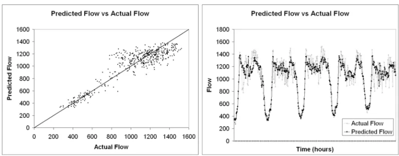
Figure 8. Scatter plot and line graph for the actual and predicted flow values for +15 minute prediction (t+1)for AURA k-NN configuration 2-1g.

Figure 9. Scatter plot and line graph for the actual and predicted flow values for +1 hour prediction (t+4)for AURA k-NN configuration 2-1g.

From figures 8 and 9 and table 6, the AURA k-NN is again smoothing transient

spikes.

4.3.3 Test 5 – the best configuration for incident detection

We repeated test 4 using the data for only the day of the traffic incident (20/06/08) which

should be anomalous and thus more difficult to predict. The overall best performing

configuration for test 5 with respect to MAPE and RMSE was identical to the best

performing configuration for test 4. We call this test 5 configuration 2-2g. As the result

replicated the result of test 4, the table of figures is omitted.

4.3.4 Test 6 – comparison to other algorithms

Test 6 compared AURA k-NN to the WEKA algorithms running identical data

configurations on data set 2. The test comprised two parts. In part 1, we used

configuration 1g from test 4 and the full week of test data. Part 2 used configuration

2-2g from test 5 and just the incident test data. The results for part 1 are listed in table 6 and

 Standard k-NN:k=10 andk=50 (to verify thatk=10 outperforms as per the AURA

k-NN).

 MLP part 1 and part 2: learning rate = 0.4, decay = true, momentum = 0.3.  SVM part 1: RBF Kernel, complexity = 150.0

 SVM part 2: RBF Kernel, complexity = 100.0.

Table 6. Table comparing the recall accuracy of the various predictors with time series length 8 and all sensors predicting a full week. The highest prediction accuracy for each row is in bold.

AURA k-NN_ 2-1gk-NN_10k-NN_50MLP SVM LMS

RMSE – 15 mins115.9 115.6 117.8 114.6116.3123.6 RMSE – 60 mins131.7 132.7 139.6 146.0155.6197.2

For part 1, the MLP had the lowest RMSE for +15 minute prediction followed by

the k-NN_10 and AURA k-NN. For +1 hour prediction, AURA k-NN was the most

accurate.

Table 7. Table comparing the recall accuracy of the various predictors with time series length 8 and all sensors predicting the day of incident only. The highest prediction accuracy for each row is shown in bold.

AURA k-NN_2- 2gk-NN_10k-NN_50MLP SVM LMS

RMSE – 15 mins128.8 128.0 137.8 137.5142.4161.9 RMSE – 60 mins150.7 151.4 157.6 163.5182.8223.4

The standard k-NN performed best for part 2 for +15 minute prediction closely

followed by the AURA k-NN and vice versa for +1 hour with AURA k-NN slightly

outperforming.

For both evaluations, usingk=10 outperformed usingk=50 for the standard k-NN

supporting our results for the AURA k-NN.

4.3.5 Test 7 – AURA k-NN run time.

Our final test was an analysis of the run time of AURA k-NN. It is vital that the

underlying prediction algorithm is able to train and predict rapidly (between data

collections) for on-line applications. Our preceding evaluations have confirmed that both

the algorithm and the data must be configured. This configuration will need to be run

periodically to maintain an up-to-date system and must be fast.

We have previously demonstrated that AURA k-NN training from raw data was

up to four times faster than conventional k-NN [21]. Zhou et al. [38] determined that the

AURA k-NN trains up to 450 times faster than an MLP. Training time is particularly

important as this forms the bulk of the overall run time. Here we evaluated whether we

k-NN may read in the data as raw data and perform training of the CMM as per section 3.

Alternatively, the contents of the CMM may be written to disk once the CMM has been

trained and then read in from the saved file. We evaluated the timings for both

approaches.

Table 8. Table listing the timings (seconds) for training the respective data sets from raw data, training the AURA k-NN from a stored CMM file and running a single query

Historical data size (vectors) Train from raw (seconds)

Train from saved (seconds)

Query (seconds)

2,976 0.268 0.0020 0.0029

29,760 9.12 0.0169 0.0086

119,040 83.9 0.0662 0.0277

1,071,360 820.4 0.5914 0.2308

The software evaluated was a C++ prototype implementation that had not been

optimised at this stage. It ran on a Linux-based 3.4Ghz Intel Pentium IV machine with

2GB of RAM and 1MB of cache. For this analysis, we used data set 2 training data

comprising 2,976 records and applied one query ofTS=8,k=10 andBins=25. We then

replicated the dataset ten times to give a training set of 29,760 records, forty times to

produce 119,040 records and 360 times to produce 1,071,360 records and recorded the

respective timings. The timings are averaged over five runs and are listed in table 8 and

shown in figure 10.

The run time growth for AURA k-NN training and querying was linear:O(n)

which agrees with our theoretical figure established in section 3. Reading the data in from

a CMM stored on disk can exploit the compact representation used for our CMM and is

almost 1400 times faster compared to training from raw data for the large 1million+

records data set. We already knew that the AURA k-NN was up to four times faster than

standard k-NN but reading the CMM from disk can further speed the AURA k-NN

markedly.

Traffic data generally arrive at five minute intervals although they may arrive as

frequently as every 30 seconds. One year of five minute interval data comprises 105,120

records. Interpolating from the above results, this would take approximately 0.07 seconds

to read from the binary file and 0.04 seconds to query. Similarly, one year of 30 second

interval data comprises 1,051,200 records which would take approximately 0.65 seconds

to read from the binary file and 0.24 seconds to query. This timing analysis indicated that

the AURA k-NN would be fast enough for our on-line IDS processing one year of

historical data, typically producing results in less than one second.

5 Analyses

K-NN in general performs comparably with other modelling approaches here with respect

to prediction accuracy as shown in tables 3, 4, 6 and 7. The advantage of the AURA

k-NN lies in the speed and scalability of training and prediction.

For algorithm configuration, the AURA k-NN only needed to optimise the

number of bins and thekvalue for each data set but these do need to be configured

carefully and a range of values assessed. This agrees with both [19] and [20] where we

also found thatthere is no single bestkvalue for predicting bus journey times [19] or a

single best number of bins for a broad range of time series data [20]. From the ten

data sets evaluated in [20] and the traffic data sets evaluated here, there is no obvious

correlation between the data characteristics and the best configuration neither is there

an obvious correlation between the data distribution and the best configuration.

Therefore, we aim to provide guidelines by recommending suitable ranges of values

forkand the number of bins. We have found that the bestkcan range from 10 to 50

here. K-NN is an instance-based learner relying on the nearest stored data points to

produce the prediction. Thekvalue is affected by the density of the data and the data

coverage. Thekvalue needs to be set to ensure that the majority of points from thek

best matches will predict the correct value. If the value is too low then the prediction

is reliant on too few data points. If it is too high then it may draw data points from

49 here. If the number of bins is set too low then the AURA k-NN will fail to

separate the data and discrimination will be too low. Too many bins and the data

points become too sparse across multiple dimensions and fail to discriminate.

The CMM does not need to be retrained to optimise thekvalue as this just

requires the number of matches returned to be varied. However, it does need retraining to

optimise the number of bins. For data configuration: the sensors, the set of attributes from

each sensor and the time series length all need to be optimised. Again, the CMM does not

need retraining to vary the sensors or attributes. If all attributes that may be used are

trained into the CMM then only CMM rows that relate to sensors under investigation

need to be activated and all other rows may be ignored.

Using more spatially distributed sensors produced better prediction accuracy as

shown by table 2 where AURA k-NN with 6 sensors outperforms AURA k-NN with 4

sensors with respect to MAPE and RMSE. Including the additional sensor attribute,

occupancy, only improved the prediction accuracy marginally (see table 2) so additional

attributes have to be selected carefully. Kamarianakis and Prastacos [18] showed that

attributes and sensors need to be carefully considered and these results agree with their

findings. Varying the time series length requires the CMM to be retrained. It was possible

to pinpoint a single ideal time series length for both data sets here (TS=8) but we expect

that the length would need to be varied for different data sets.

Previous evaluation have shown that AURA k-NN trains from raw data up to 450

times faster than an MLP [38] and executes up to four times faster than standard k-NN

[21]. Here, we showed in table 8 that AURA k-NN executed even more rapidly by

reading trained CMMs stored on disk and then retrieving theknearest neighbours.

An advantage of both standard and AURA k-NN over the model-based

approaches is that they can incorporate new data into the k-NN framework simply and

quickly. New data may simply be added to the database for standard k-NN or added as

new columns to the AURA CMM. A model-based approach would have to remodel the

new data which is a computationally intensive process. The AURA k-NN will need to be

tuned periodically to keep it up to date but evaluating multiple algorithm and data

configurations is computationally feasible. Conversely, the SVM and MLP require

intensive optimisation across a number of parameters and we noticed that the RMSE for

both the SVM and the MLP varied according to the parameters selected. This presents

computational processing issues for an on-line IDS using either an SVM or MLP as the

data would need to be remodelled regularly as new data became available to prevent

model drift.

We noted in our four criteria that the prediction algorithm must be able to

Caprara [39] suggested that multivariate k-NN can identify chaotic time series patterns

(such as those found in traffic flows) that model-based approaches would miss. The

nonparametric regression technique of k-NN which effectively mines the data and

retrieves actual cases (local search) is much better suited to such prediction tasks than

data modelling techniques such as MLP, SVM or LMS which produce general models

that tend towards the mean. Data such as traffic flows are susceptible to local, short-term

variations such as daily variations in demand, incidents or the weather. These short-term

variations must be identifiable by the technique to allow accurate prediction and a model

that tends towards the mean may well miss them. This hypothesis agrees with the findings

of [17, 39, 40] across various problem domains.

The AURA k-NN will generate a prediction using the average value of thek

neighbours. This averaging tended to smooth transient spikes and appeared to be

overestimating more frequently than underestimating for this data. However, the data sets

used in these evaluations were relatively small. We posit that a larger training set, such as

a full year of data with 365 * 96 = 35,040 records (assuming no missing data), may lead

to more accurate predictions as more examples of each time series would be present.

6 Conclusion

The AURA k-NN was the overall best performing predictor of the methods evaluated on

the data sets in this paper in terms of both speed and accuracy. It performs comparably

with respect to prediction accuracy and is able to be implemented for rapid execution and

scalability of both training and retrieval of theknearest neighbours. We envisage using

the AURA k-NN as a “train once use many” predictor, writing the CMM to disk for

safety, running repeated queries and reading the CMM from disk when necessary. New

data may be added to the CMM by adding additional columns to the matrix. The rapid

execution allows the algorithm and data parameters to be tuned if necessary to prevent

drift.

All predictors evaluated here required both the data and algorithm settings to be

configured. The fast execution time and minimal parameter set of the AURA k-NN

facilitates this combinatorial configuration process. The only algorithm parameter

required for standard k-NN is thekvalue. The AURA k-NN added one parameter to this:

the number of quantisation bins for each attribute. It may be possible that heuristics to

guide the parameter setting can be inferred through analysing a diverse range of data sets.

One disadvantage of k-NN is that it is only as good as the historical data in the

database. Some model based methods such as MLPs are able to generalise and effectively

plug gaps in the training data. If there is a gap in the data space then there will be no

distant neighbours. Hence, it is vital, that the historical data base is sufficiently large with

sufficient coverage to optimise accuracy. This is particularly true for infrequent events

such as traffic incidents. A large database covering a long time span will contain more

event data which will enable better instance-based prediction for a k-NN method.

However, if the data base is too large then computational time will be excessive for

standard k-NN. For this reason, we use the faster AURA k-NN to underpin the predictor

so much larger databases with better coverage may be processed.

We feel that the AURA k-NN prediction accuracy can be improved. We noted

from the MPE that the AURA k-NN tends to overestimate traffic flows. Hence, future

work will investigate increasing the prediction accuracy by incorporating: time-of-day

matching using time-of-day profiles; k-NN distance weighting; and, introducing error

feedback. As discussed above, using a larger database covering a longer time span may

also improve instance-based prediction. We will also investigate using confidence

estimators where the prediction is accompanied by a confidence value based on the

distance of the matches from the query.

Ultimately, it is hoped that the predictor will be incorporated into an intelligent

decision support system for traffic monitoring and tested against real-world data from

London, Kent and York in the UK. By producing predictions, the IDS will be able to

make recommendations proactively and anticipate traffic problems rather than

functioning reactively and being subject to time lags inherent in data collection. The

proposed method is generic and we hope to apply it to other domains that use spatially

distributed sensors where neighbourhoods of sensors exist and where temporal

characteristics are important.

Acknowledgments

The work reported in this paper forms part of the FREEFLOW project, which is supported by the UK Engineering and Physical Sciences Research Council, the UK Department for Transport and the UK Technology Strategy Board. The project consortium consists of partners including QinetiQ, Mindsheet, ACIS, Kizoom, Trakm8, City of York Council, Kent County Council, Transport for London, Imperial College London and University of York.

References

[1] Gorry, G. and Scott-Morton, M. (1971). A framework for management information systems. Sloan Management Rev., 13(1):55-70.

[3] Schelter, B., Winterhalder, M. and Timmer, J. (2006). Handbook of time series analysis: recent theoretical developments and applications, Wiley-VCH, ISBN: 978-3-527-40623-4

[4] Ding, A., Zhao, X. and Jiao, L. (2002). Traffic Flow Time Series Prediction Based On Statistics Learning Theory. In, Procs IEEE 5th International Conference on Intelligent Transportation Systems, pp. 727-730.

[5] Vapnik, V. (1995). The nature of statistical learning theory. New York: Springer-Verlag, ISBN: 0387987800.

[6] Box, G. and Jenkins, G. (1976). Time Series Analysis: Forecasting and Control. Holden-Day, San Francisco.

[7] Hamed, M. and Al-Masaeid, H. (1995). Short-term prediction of traffic volume in urban arterials. J. of Transp. Eng. (ASCE) 121(3): 249-254.

[8] Williams, B., Durvasula, P. and Brown, D. (1998). Urban freeway traffic flow prediction: Application of seasonal autoregressive integrated moving average and exponential smoothing models. Transp. Res. Record: J. of the Transp. Res. Board, 1644: 132-141.

[9] Ghosh, B., Basu, B. and O'Mahony, M. (2007). Bayesian time-series model for short-term traffic flow forecasting. Journal of Transp. Eng. (ASCE) 133(3): 180-189.

[10] Amin, S., Rodin, E., Liu, A-P. and Rink, K. (1998). Traffic Prediction and Management via RBF Neural Nets and Semantic Control. J. of Computer-Aided Civ. and Infrastruct. Eng., 13: 315-327.

[11] Vlahogianni, E., Karlaftis, M. and Golias, J. (2005). Optimized and meta-optimized neural networks for short-term traffic flow prediction: A genetic approach. Transp. Res. Part C: Emerging Technologies, 13(3): 211-234.

[12] Abdulhai, B., Porwal, H. and Recker, W. (2002). Short-Term Traffic Flow Prediction Using Neuro-Genetic Algorithms. J. of Intell. Transp. Sys.: Technology, Planning, and Operations, 7(1): 3-41: Taylor & Francis.

[13] Martinetz, T., Berkovich, S. and Schulten, K. (1993). Neural-gas network for vector

quantization and its application to time-series prediction. IEEE-Trans. on Neural Netw., 4(4): 558-569.

[14] Zhang,C., Sun,S. and Yu, G. (2004). Short-Term Traffic Flow Forecasting Using Expanded Bayesian Network for Incomplete Data. In, Procs International Symposium on Neural Networks, Dalian, China. Lecture Notes in Computer Science, (LNCS 3174), Springer-Verlag.

[15] Kindzerske M. and Ni, D. (2007). A Composite Nearest Neighbor Nonparametric Regression to Improve Traffic Prediction. Transp. Res. Record:J. of the Transp. Res. Board, 1993: 30-35. [16] Yakowitz, S. (1987). Nearest-Neighbour Methods for Time Series Analysis. J. of Time Series Anal., 8(2): 235-247.

[18] Kamarianakis, Y. and Prastacos, P. (2003). Forecasting traffic flow conditions in an urban network: Comparison of multivariate and univariate approaches. Transp. Res. Record: J. of the Transp. Res. Board, 1857: 74-84.

[19] Hodge, V., Jackson, T. and Austin, J. (2012).A Binary Neural Network Framework for Attribute Selection and Prediction. In, Procs 4th International Conference on Neural Computation Theory and Applications (NCTA 2012), pp. 510-515, Barcelona, Spain: SciTePress

[20] Hodge, V. and Austin, J. (2012). Discretisation of Data in a Binary Neural k-Nearest

Neighbour Algorithm. Tech Report YCS-2012-473, Department of Computer Science, University of York, UK

[21] Hodge, V. and Austin, J. (2005). A Binary Neural k-Nearest Neighbour Technique. Knowl. and Inf. Sys., 8(3): 276–292, Springer-Verlag London Ltd.

[22] Austin, J., Kennedy, J. and Lees, K. (1998). The Advanced Uncertain Reasoning

Architecture, AURA. In, RAM-based Neural Networks, Ser. Progress in Neural Processing. World Scientific Publishing, 9: 43-50.

[23] Hodge, V., Krishnan, R., Austin, J. and Polak, J. (2010). A computationally efficient method for online identification of traffic incidents and network equipment failures. Presented at, 3rd Transport Science and Technology Congress: TRANSTEC 2010, New Delhi, April 4-7, 2010. [24] Krishnan, R., Hodge, V., Austin, J. and Polak, J. (2010a) A Computationally Efficient Method for Online Identification of Traffic Control Intervention Measures. 42ndAnnual UTSG Conference, Centre for Sustainable Transport, University of Plymouth, UK: January 5-7, 2010 [25] Krishnan, R., Hodge, V., Austin, J., Polak, J. and Lee, T-C. (2010b). On Identifying Spatial Traffic Patterns using Advanced Pattern Matching Techniques. In, Transportation Research Board (TRB) 89th Annual Meeting, Washington, D.C., January 10-14, 2010. ( DVD-ROM: 2010 TRB 89th Annual Meeting: Compendium of Papers)

[26] Hebb, D. (1949). The organization of behavior: a neuropsychological theory, Wiley, New York.

[27] Hodge, V. and Austin, J. (2001). An evaluation of standard retrieval algorithms and a binary neural approach. Neural Netw., 14(3): 287-303

[28] Bentz, H., Hagstroem, M. and Palm, G. (1989). Information storage and effective data retrieval in sparse matrices. Neural Netw., 2(4): 289–293.

[29] Austin, J. (1995). Distributed associative memories for high speed symbolic reasoning. In, R. Sun and F. Alexandre, (eds), IJCAI ’95 Working Notes of Workshop on

Connectionist-Symbolic Integration: From Unified to Hybrid Approaches, pp. 87–93, Montreal, Quebec.

[30] Weeks, M., Hodge, V., O'Keefe, S., Austin, J. & Lees, K. (2003). Improved AURA k-Nearest Neighbour Approach. In, Procs IWANN-2003, International Work-conference on Artificial and Natural Neural Networks, Mahon, Spain. June 3-6, 2003. Lecture Notes in Computer Science (LNCS) 2687, Springer Verlag, Berlin.

[31] Hall, M., Frank, E., Holmes, G., Pfahringer, B., Reutemann, P. and Witten I. (2009). The WEKA Data Mining Software: An Update. ACM SIGKDD Explorations Newsletter, 11(1): 10-18. [32] Witten, I. and Frank, E. (2005). Data Mining: Practical Machine Learning Tools and

[33] Cover T. and Hart P. (1967). Nearest neighbor pattern classification. IEEE Trans on Information Theory, 13(1): 21–27.

[34] Rumelhart, D., Hinton, G. and Williams, R. (1988). Learning representations by back-propagating errors (pp. 696-699). MIT Press, Cambridge, MA, USA.

[35] Platt, J. (1998). Fast Training of Support Vector Machines using Sequential Minimal Optimization. In, B. Schoelkopf, C. Burges and A. Smola, (eds), Advances in Kernel Methods -Support Vector Learning. MIT Press, Cambridge, MA, USA, 185-208.

[36] Labeeuw, W., Driessens, K., Weyns, D., Holvoet, T. and Deconinck, G. (2009). Prediction of Congested Tra c on the Critical Density Point Using Machine Learning and Decentralised Collaborating Cameras. In, New Trends in Artificial Intelligence, 14th Portuguese Conference on Artificial Intelligence, EPIA 2009, Aveiro, Portugal, pp. 15-26.

[37] Krishnan, R., (2008). Travel time estimation and forecasting on urban roads, PhD thesis, Centre for Transport Studies, Imperial College London.

[38] Zhou, P., Austin, J. and Kennedy, J. (1999). High Performance k-NN Classifier Using a Binary Correlation Matrix Memory. In, Procs Advances in Neural Information Processing Systems Vol. II, David A. Cohn (Ed.). MIT Press, Cambridge, MA, USA, 713-719.

[39] Mulhern, F. and Caprara, R. (1994). A Nearest Neighbor Model for Forecasting Market Response. Int. J. of Forecast., 10(2): 191-207, ISSN 0169-2070.