An analytical method for the optimisation of weakly nonlinear systems

This is a repository copy of

An analytical method for the optimisation of weakly nonlinear

systems

.

White Rose Research Online URL for this paper:

http://eprints.whiterose.ac.uk/80984/

Proceedings Paper:

Hill, T.L., Cammarano, A., Neild, S.A. et al. (1 more author) (2014) An analytical method for

the optimisation of weakly nonlinear systems. In: Proceedings of EURODYN 2014.

EURODYN 2014 9th International Conference on Structural Dynamics, 30 June – 2 July

2014, Porto, Portugal. , 1981 - 1988. ISBN 978-972-752-165-4

Reuse

Unless indicated otherwise, fulltext items are protected by copyright with all rights reserved. The copyright exception in section 29 of the Copyright, Designs and Patents Act 1988 allows the making of a single copy solely for the purpose of non-commercial research or private study within the limits of fair dealing. The publisher or other rights-holder may allow further reproduction and re-use of this version - refer to the White Rose Research Online record for this item. Where records identify the publisher as the copyright holder, users can verify any specific terms of use on the publisher’s website.

Takedown

If you consider content in White Rose Research Online to be in breach of UK law, please notify us by

An analytical method for the optimisation of weakly nonlinear systems

T.L. Hill1_{, A. Cammarano}1_{, S.A. Neild}1_{, D.J. Wagg}2

1_{Department of Mechanical Engineering, University of Bristol, Bristol, BS8 1TR, UK} 2_{Department of Mechanical Engineering, University of ShefÞeld, ShefÞeld, S1 3JD, UK}

email: [email protected], [email protected], [email protected], david.wagg@shefÞeld.ac.uk

ABSTRACT: In this paper we discuss how backbone curves can be used to guide the design and optimisation of weakly nonlinear systems with multiple degrees-of-freedom. After decomposing the system using the modes of the equivalent linear system (the linear modes), we show how the backbone curves of the unforced, undamped equivalent system can be calculated. These consist of pure responses in each of the linear modes and, in certain parameter regimes, responses which are a combination of two or more linear modes - a feature which can be linked to internal resonance. Using an example system we will investigate how these backbone curves can be used to describe particular characteristics of the response. An energy balancing technique is also employed to relate the backbone curves to the response of the forced and damped system, and anticipate the conditions for which a particular characteristic will be seen. Finally, we discuss how the analytical nature of these techniques enables us to precisely design and optimise characteristics of such systems and how this can be expanded to systems with a greater number of degrees-of-freedom.

KEY WORDS: Nonlinear dynamics; Backbone curves; Second-order normal forms; Energy balancing.

1 INTRODUCTION

A major challenge for structural engineers is dealing with nonlinear behaviours. The demand for lighter and more efÞcient structures brings with it a requirement that structures operate beyond the limits where linearity may be assumed. To design structures with nonlinear characteristics, engineers must be able to predict their response and understand how these charac-teristics may be exploited and designed into structures. One existing approach to modelling nonlinear dynamic behaviour is using numerical continuation programmes, such as AUTO-07p [1], which provides an accurate solution to the differential equations describing the system. However this provides little insight into the relationships between the characteristics of the system and the response and becomes increasingly complex and involved for large systems, making it unsuitable for many practical applications.

Analytical and semi-analytical techniques provide greater insight into the relationships within systems and offer greater scalability. Nonlinear normal modes, see [2] and [3], are one such technique and can provide insight into the behaviour of nonlinear structures, and their resonant interactions. Ap-proaches such as perturbation and harmonic balance techniques [4] provide good, analytical approximations to weakly nonlinear systems, although they also become increasingly complex with scale and thus ill-suited for large systems. Methods for automating these techniques do allow for an expansion in the complexity of the systems they are used to model, see for example [5] and [6].

In this work an approach based on the second-order normal form technique is presented. This is used to not only describe the response of the nonlinear system, but also to derive expressions relating the behaviours in the response to the physical parameters describing the system. This allows

for the development of expressions that may be used for the optimisation of systems operating in the nonlinear regime. The backbone curves, describing the response of the unforced, undamped equivalent system, provide a simple description of the system and hence are used in this work as a starting point. They also highlight the interactions that may occur within the system whilst relating to the behaviour of the response when the system is forced and damped.

Section 2 gives a step-by-step description of the application of the second-order normal form technique when used to calculate the backbone curves for systems with multiple-degrees-of-freedom (MDOF), and the motivation for each transform is explained. In Section 3, this approach is demonstrated for a two-mass oscillator with a nonlinear spring, where the nonlinear component is described by a single parameter. This results in a set of expressions describing the backbone curves of the system, which are then used to derive expressions for the relationship between particular aspects of the response of the system and the nonlinear parameter. Section 4 introduces an energy-based technique which allows the relationship between the backbone curves and the forced response to be speciÞed. These descriptions of the dynamics of the system are then combined in Section 5, where the system is optimised. Conclusions are then drawn in Section 6.

2 THE SECOND-ORDER NORMAL FORM TECHNIQUE The second-order normal form technique allows the behaviour of weakly nonlinear systems to be described analytically; where here, analytical solutions are also assumed to be approximate. This enables the design and optimisation of the response of such systems based on their physical characteristics, making it a valuable tool for the analysis considered here. This technique is applied directly to systems described in the second-order differential form; a more natural formulation of engineering A. Cunha, E. Caetano, P. Ribeiro, G. Müller (eds.)

problems. This gives advantages over the Þrst-order (state-space based) approach [7] with regard to both the ease of formulation, and improved accuracy [9]. The approach also has advantages over numerical techniques, such as continuation approaches (for example AUTO-07p, [1]) and nonlinear normal modes (where an analytical solution can only be found in certain circumstances), see for example [2] and [3]. The second-order normal form technique is limited to smooth, lightly damped, weakly-nonlinear systems – i.e. systems operating in regimes where the nonlinear (and damping) terms are small in comparison to the undamped linear terms.

A number of works describe the technique, for example [8], [9] and [10], for a broad range of systems. For completeness, a description is given of the application of the technique to the class of system considered here (i.e. for computation of the backbone curves of MDOF systems).

2.1 PROBLEM FORMULATION

Consider a forced and damped nonlinear system withN degrees-of-freedom, whose equation of motion can be written

M¨x+Cxú+Kx+ΓΓΓx(x) =Pxcos(Ωt), (1)

where: x is an N_×1 vector of displacements; M, C and K areN_×N mass, damping and stiffness matrices respectively; ΓΓΓx(x)is anN×1 vector of nonlinear terms; andPxis anN×1

vector of forcing amplitudes. Note thatΓΓΓx(x)is a function of

displacement only – i.e. the system has no nonlinear damping or forcing. ToÞnd the backbone curves of this system, we require the underlying conservative system, which may be written

M¨x+Kx+ΓΓΓx(x) =0. (2)

2.2 LINEAR MODAL TRANSFORM(x→q)

The system described by Eq. (2) can now be projected onto the underlying linear system by applying the linear modal transform x=ΦΦΦq. Here, ΦΦΦ is an N_×N matrix where the nth column describes the modeshape of thenth linear mode. These can be found as the eigenvectors ofM−1K, where the corresponding eigenvalues areω2

nn(the square of the natural frequency of the

nth linear mode). This transform leads to the modal dynamic equation

¨

q+ΛΛΛq+Nq(q) =0, (3)

whereΛΛΛis anN_×Ndiagonal matrix wherenthleading diagonal element isω2

nn.

In its typical formulation, the next step of the second-order normal form technique is the forcing transform, which removes all forcing terms that are not close to the response frequencies of the linear modes. As this formulation only concerns unforced systems, this step is omitted.

2.3 NONLINEAR NEAR-IDENTITY TRANSFORM(q_→u)

The Þnal step in the technique is the nonlinear near-identity transform. Here, the transform q=u+h(u) is applied to Eq. (3), leading to

¨

u+ΛΛΛu+Nu(u) =0. (4)

Here,uis anN_×1 vector describing the fundamental response ofq, andh is anN_×1 vector containing all of the harmonic

contents of q. By deÞningh as a function ofu(i.e. treating the harmonic contents of the response as a function of the fundamental response) we may determine the total response ofq from a solution foru. In this transform we requirehto be small, such that the transform is near-identity. Usingε, a bookkeeping parameter denoting smallness, we may write h as h=εh,ˆ indicating the smallness of h. By applying a power series expansion inε, we may writehash=εhˆ1+ε2hˆ2+ε3hˆ3+...,

from which we can approximateh_≈h1. As we are assuming

the nonlinear terms to be small (i.e.Nq=εNˆqandNu=εNˆu),

we can also make the approximationsNq≈nq1andNu≈nu1.

We may nowÞnd a solution for Eq. (4) using the substitution for thenthelement ofu

un = Uncos(ωrnt−φn),

= unp+unm=

Un

2

e+j(ωrnt−φn)_+e−j(ωrnt−φn)_{, (5)}

whereUn,ωrnandφnare the amplitude, frequency and phase of

the responseun. The subscriptspandmdenote the positive and

negative powers of the exponentials respectively. Note that the response frequency,ωrn, ofunis distinct from the linear natural

frequency,ωnn, ofqn.

We now make the approximationq=u=up+um, true to

Þrst-order accuracy ashis small, an substitute this into Eq. (3). From this we can deÞne theL_×1 vectoru∗(up,um), containing

theLunique combinations ofup andum. We may also deÞne

theN_×Lmatrices[nq],[nu]and[h]containing all coefÞcients of

the terms inu∗, such that

nq1= [nq]u∗, nu1= [nu]u∗, h1= [h]u∗. (6)

Theℓthelement ofu∗can be written u∗_ℓ =

N

∏

n=1

{usnpnℓpusnmnℓm}. (7)

From this we can determine which terms resonate at the response frequenciesωrn. These terms will contribute to the

fundamental response,u, whilst the non-resonant terms will be stored in the vector of harmonic componentsh. The resonant terms can be determined as the elements in theN_×Lmatrixβββ with a value of zero. Element(n, ℓ)ofβββ is calculated as

βnℓ=

N

∑

k=1

(sℓk p−sℓkm)ωrk

2

−ωrn2, (8)

wheresℓk pandsℓkmare deÞned in Eq. (7). Now, the elements in

[nu]and[h]corresponding to those inβββ can be calculated as

βnℓ=0 → nu,nℓ=nq,nℓ & hnℓ=0, (9a) βnℓ=0 → nu,nℓ=0 & hnℓ=nq,nℓ/βnℓ. (9b)

From Eq. (6) we can now use [nu] and u∗ to Þnd nu1, and

henceNu. Substituting this into Eq. (4) we can then calculateu.

ToÞnd the harmonic content, we can substitute the calculated values ofuinto the expression forh(found using Eqs. (6) and (9)). The total modal response can then be found using q= u+h, and the response in the physical coordinates is calculated byx=ΦΦΦq.

m m

k1 k2 (k1,κ)

c1 c2 c1

Pcos(Ωt) x1 Pcos(Ωt) x2

Figure 1. Schematic diagram of a two-degree-of-freedom oscillator. The underlying unforced, linear system is symmetric and a nonlinearity creates an asymmetry.

3 EXAMPLE: A TWO DEGREE-OF-FREEDOM SYSTEM Figure 1 shows a forced, damped system with two degrees-of-freedom. The underlying linear, conservative system is symmetric, the damping is symmetric and linear, and the forcing is antisymmetric. The spring connecting the second mass to ground is nonlinear, creating an asymmetry in the system. This is a DufÞng-type spring with the force-deßection relationship F=k1(Δx) +κ(Δx)3, where (Δx)is the displacement of the

spring. The linear spring grounding theÞrst mass has spring constantk1, and the linear dampers connecting the masses to

ground both have damping constants c1. The linear spring

and damper connecting the two masses have constantsk2 and

c2 respectively. A sinusoidal forcing, with amplitude P at

frequencyΩ, acts on both masses, but in anti-phase. This is equivalent to writing the forcing amplitudes acting on theÞrst and second mass asP1=PandP2=−Prespectively.

For the system considered, we use the parameter values

m=1, k1=1, k2=0.105,

P=0.005, c1=0.005, c2=0.005, (10)

whilstκ>0 and may be varied. This system may be described in the form of Eq. (1) where

M=

1 0

0 1 , C=

0.01 −0.005

−0.005 0.01 ,

K=

1.105 ₋0.105

−0.105 1.105 , ΓΓΓx=

0 κx3₂

, (11)

Px=

0.005

−0.005

cos(Ωt). (12)

Finding the eigenvalues and eigenvectors ofM−1K, results in ΛΛΛ=

1 0

0 1.21 , ΦΦΦ=

1 1

1 ₋1 . (13)

Hence, the linear natural frequencies areωn1=1 andωn2=1.1.

Now, performing the linear modal transform results in

¨

q+ΛΛΛq+Nq=Pq, (14)

where:

Nq =

+1

−1 κ_(q

1−q2)3

2m +

0.005 0 0 0.015 qú,

Pq =

0 0.005

cos(Ωt). (15)

Here, the damping and forcing terms have been included for use in the energy balancing technique considered later. First, however, the backbone curves of this system are calculated, in order to identify the underlying behaviour. This is achieved by neglecting the forcing and damping terms, and substitutingqn≈

un=unp+unm, such that

Nq=κ(

u1p+u1m−u2p−u2m)3

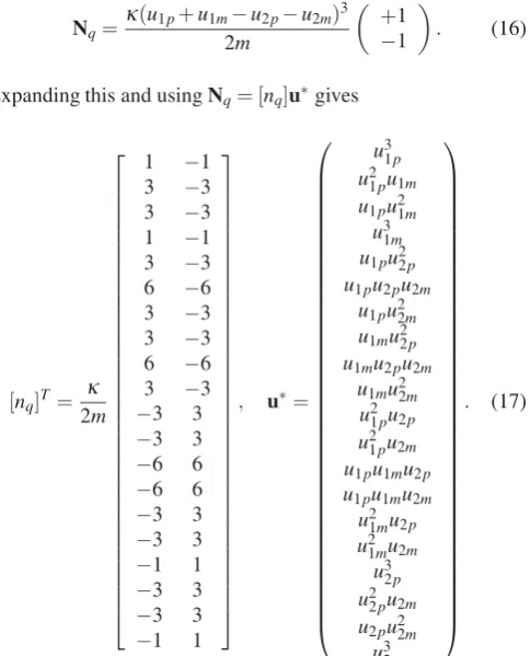
2m +1 −1 . (16)

Expanding this and usingNq= [nq]u∗gives

[nq]T= κ

2m ⎡ ⎢ ⎢ ⎢ ⎢ ⎢ ⎢ ⎢ ⎢ ⎢ ⎢ ⎢ ⎢ ⎢ ⎢ ⎢ ⎢ ⎢ ⎢ ⎢ ⎢ ⎢ ⎢ ⎢ ⎢ ⎢ ⎢ ⎢ ⎢ ⎢ ⎢ ⎢ ⎢ ⎢ ⎣

1 ₋1 3 −3 3 ₋3 1 ₋1 3 −3 6 −6 3 ₋3 3 ₋3 6 −6 3 ₋3

−3 3

−3 3

−6 6

−6 6

−3 3

−3 3

−1 1

−3 3

−3 3

−1 1 ⎤ ⎥ ⎥ ⎥ ⎥ ⎥ ⎥ ⎥ ⎥ ⎥ ⎥ ⎥ ⎥ ⎥ ⎥ ⎥ ⎥ ⎥ ⎥ ⎥ ⎥ ⎥ ⎥ ⎥ ⎥ ⎥ ⎥ ⎥ ⎥ ⎥ ⎥ ⎥ ⎥ ⎥ ⎦

, u∗= ⎛ ⎜ ⎜ ⎜ ⎜ ⎜ ⎜ ⎜ ⎜ ⎜ ⎜ ⎜ ⎜ ⎜ ⎜ ⎜ ⎜ ⎜ ⎜ ⎜ ⎜ ⎜ ⎜ ⎜ ⎜ ⎜ ⎜ ⎜ ⎜ ⎜ ⎜ ⎜ ⎜ ⎜ ⎜ ⎜ ⎝

u3_1p u2_1pu1m

u1pu21m

u3_1m u1pu22p

u1pu2pu2m

u1pu22m

u1mu22p

u1mu2pu2m

u1mu22m

u2_1pu2p

u2_1pu2m

u1pu1mu2p

u1pu1mu2m

u2_1mu2p

u2_1mu2m

u3_2p u2_2pu2m

u2pu22m

u3_2m ⎞ ⎟ ⎟ ⎟ ⎟ ⎟ ⎟ ⎟ ⎟ ⎟ ⎟ ⎟ ⎟ ⎟ ⎟ ⎟ ⎟ ⎟ ⎟ ⎟ ⎟ ⎟ ⎟ ⎟ ⎟ ⎟ ⎟ ⎟ ⎟ ⎟ ⎟ ⎟ ⎟ ⎟ ⎟ ⎟ ⎠ . (17)

Asωn1andωn2are close, it is assumed that the two modes will

respond at the same frequency, which we will denote atΩ(i.e. Ω=ωr1=ωr2). Fromu∗, and using Eq. (8), we calculateβββas

βββT _=Ω2

The zero terms inβββ satisfy the condition given by Eq. (9a), which we use to Þnd the matrix [nu], and using Eq. (6) the

nonlinear components of the fundamental response are found to be

nu1= 3κ

2m _(2u

2pu2m+u1pu1m)u1+u1pu22m+u1mu22p

(2u1pu1m+u2pu2m)u2+u21pu2m+u21mu2p

−(2u1pu1m+u2pu2m)u2−u21pu2m−u21mu2p

−(2u2pu2m+u1pu1m)u1−u1pu22m−u1mu22p

. (18)

This may be written in the form

nu1=n˜u1e+jΩt+n¯u1e−jΩt, (19)

where ˜nu1 and ¯nu1 are complex conjugates. Substituting the

expansions ofunpand unm, given in Eq. (5), and using φd =

φ1−φ2, the ˜nu1component may be written

˜

nu1=_16m3κ

U₁2+

2+e+j2φd

U₂2₋U₁−1U₂3e+jφd

2+e−j2φd

U₁2+U₂2₋U₁3U₂−1e−jφd

−

2e+jφd_+e−jφd

U1U2U1e−jφ1

−

2e−jφd₊e+jφd_U1U2U2e−jφ2

. (20)

Substituting this into Eq. (4), and usingNu≈nu1and ¨u=−Ω2u,

weÞnd that Eq. (4) may be separated into complex conjugate parts, akin to Eq. (19). Taking the conjugate part corresponding to e+jΩt_gives

1 2

_ω2

n1−Ω2

U1e−jφ1

_ω2

n2−Ω2

U2e−jφ1

e+jΩt_+n˜

u1e+jΩt=

0 0

, (21)

which can be rearranged to

ω2

n1−Ω2+

3κ 8m

U₁2+2+e+j2φdU₂2₋U₁−1U₂3e+jφd

−2e+jφd_+e−jφd U1U2

U1e−jφ1=0, (22a)

ω2

n2−Ω2+

3κ 8m

2+e−j2φdU₁2+U₂2₋U₁3U₂−1e−jφd

−2e−jφd_+e+jφd_U1U2U2e−jφ2_{=0. (22b)} AssumingU1=0 andU2=0 this can be written

ωd1+3κ

8m

U₁2+2+e+j2φdU₂2₋U₁−1U₂3e+jφd

−2e+jφd_+e−jφd U1U2

=0, (23a)

ωd2+

3κ 8m

2+e−j2φd_U2

1+U22−U13U2−1e−jφd

−2e−jφd+e+jφdU1U2

=0, (23b)

where we have used

ωd1=ωn21−Ω2, and ωd2=ωn22−Ω2. (24)

Taking the imaginary parts of Eqs. (23) leads to

U₂2sin(2φd)−U1U2sin(φd)−U1−1U23sin(φd) =0, (25a)

U12sin(2φd)−U1U2sin(φd)−U13U2−1sin(φd) =0, (25b)

which may be satisÞed by either

sin(φd) =sin(φ1−φ2) =0, (26a)

or cos(φd) =cos(φ1−φ2) =

U₁4₋U₂4 2U1U2(U12−U22)

. (26b)

Taking the real parts of Eqs. (23) leads to

ωd1+3κ

8m

U₁2+ (cos(2φd) +2)U22

−

3U1U2+U1−1U23

cos(φd)=0, (27a)

ωd2+_8m3κU22+ (cos(2φd) +2)U12

−

3U1U2+U13U2−1

cos(φd)=0. (27b)

From this it can be found that the phase relationship described by Eq. (26b) cannot be satisÞed. Hence, from Eq. (26a), the phase difference betweenu1andu2on the backbone curves is

|φd|=|φ1−φ2|=0,π. (28)

We now deÞnep=cos(φd)wherep= +1 describes backbone

curves where|φd|=0, and p=−1 describes backbone curves

where_|φd|=π. This allows Eqs. (27) to be written

ωd1U1+3κ

8m[U1−pU2]

3_{=0, (29a)}

ωd2U2−p3κ

8m[U1−pU2]

3

=0, (29b)

which leads to the relationship betweenU1andU2

U1=−pω_ωd2

d1U2. (30)

Recalling Eqs. (24), and using the restriction that bothU1andU2

must be real and positive, we can conclude that p= +1 when ωn1<Ω<ωn2andp=−1 in all other cases. Next, substituting

Eq. (30) into Eq. (29a) leads to

ωd2+3κ

8m ω

d2

ωd1+1 3

U₂2=0, (31)

henceU2may be determined using

U₂2=−8mωd2 3κ

ω

d1

ωd1+ωd2

3

, (32)

showing thatU2 is independent of p. ForU2 to be real, and

assumingκ>0, we require

ωd2

ω

d1

ωd1+ωd2

3

<0. (33)

There are three cases to consider. Firstly whenΩ>ωn2,ωd1<0

andωd2<0, applying Eq. (33) leads to

ωd1

ωd1+ωd2 >

0, (34)

WhenΩ<ωn1,ωd1>0 andωd2>0, applying Eq. (33) gives

ωd1

ωd1+ωd2 <0, (35)

which cannot be satisÞed.

Whenωn1<Ω<ωn2,ωd1<0 andωd2>0, applying Eq. (33)

leads to _ω

d1

ωd1+ωd2 <0, (36)

which requires thatωd1+ωd2>0. Substituting Eqs. (24) and

rearranging gives the inequality

Ω< 1/2_ω2

n1+ωn22

. (37)

Hence, backbone curves only exist when ωn1 < Ω <

1/2ω₂

n1+ωn22

andΩ>ωn2.

If the harmonic content of the response is small (i.e. h is small) then we may make the approximationq_≈u(see Section 2.3). Using the relationships x1 =q1+q2 and x2 =q1−q2

determined from the linear modal transform (see Section 2.2) we can then make the approximationsx1≈u1+u2andx2≈u1−u2.

Asu1andu2are both responding at frequencyΩ:X1≈U1+U2

andX2≈ |U1−U2|whenu1andu2are in-phase (i.e.p= +1);

X1≈ |U1−U2|andX2≈U1+U2whenu1andu2are anti-phase

(i.e.p=−1). Using Eq. (30), these can be written:

p= +1 : X1≈

1−ω_ωd2

d1

U2, X2≈

! ! ! !1+

ωd2

ωd1

! ! ! !

U2, (38a)

p=−1 : X1≈

! ! ! !

1₋ωd2 ωd1

! ! ! !

U2, X2≈

1+ω_ωd2

d1

U2. (38b) Therefore the physical coordinate amplitudes may be written

X1≈

! ! ! !1−

ωd2

ωd1

! ! ! !

U2, X2≈

! ! ! !1+

ωd2

ωd1

! ! ! !

U2, (39)

regardless of the value ofp. Combining this with Eqs. (24) and (32), leads to

X1=

! ! ! !

ω2 n1−ωn22

ω2 n1−Ω2

! ! ! !

U2, X2=

! ! ! !

ω2

n1+ωn22−2Ω2

ω2 n1−Ω2

! ! ! !

U2, (40a)

where U2=

" 8m_Ω2

−ωn22

3κ

ω2 n1−Ω2

ω2

n1+ωn22−2Ω2

3

.(40b)

From this we can calculate the backbone curves in the projection of the response frequency,Ω, against the physical coordinates, X1 and X2, as shown in Figure 2. The backbone curves

originating at Ω = 1 and Ω =1.1 are labelled S1 and S2 respectively. It can be seen that S1 tends asymptotically to Ω= 1/2_ω2

n1+ωn22

≈1.0512, and that no backbone curve exists between 1.0512<Ω<1.1, as predicted.

The backbone curves of a system are representative of its underlying behaviour, and the forced response of the system will tend to envelope them. This allows conclusions regarding the forced response of the system to be drawn from the backbone curves. It is found thatS1has a composition dominated by the

Þrst linear mode,q1. As this system is forced purely inq2– see

1 1.1 1.2 1.3

0 0.1 0.2 0.3 0.4

S1

S2

Ω

X

1

1 1.1 1.2 1.3

0 0.1 0.2 0.3 0.4

S1

S2

Ω

X

2

Figure 2. Backbone curves of the system whenκ=5 in the projection of response frequency,Ω, against displacement amplitude of theÞrst and second mass,X1andX2, in panels

(a) and (b) respectively.

Eq. (15) – we can conclude that this forced response has only a weak tendency to envelope this backbone curve. Meanwhile S2 is composed primarily ofq2, making the forced response

strongly attracted to it. S2shows the properties of a response that is well suited for use as a vibration absorber or energy harvester, as the response amplitude of theÞrst mass,X1, is held

at a low value across a large bandwidth, whilstX2the response is

high, showing that most of the energy is held in the second mass. Although the response ofX1is high inS1, the weak attraction of

the forced response to this backbone curve means that this high amplitude should be avoided.

4 ENERGY BALANCING

to the forcing and damping terms in the equation of motion of the system, must be zero over one period. This must be true for all steady-state solutions in the forced response; however it requires trial solutions that are compatible with the remaining terms. Making the assumption that the forced response crosses the backbone curves, the backbone curves provide a set of trial solutions meeting this requirement. Therefore any points on the backbone curves that satisfy this energy balancing requirement must also represent a point crossed by the forced response.

For the system considered in Section 3, projected onto the linear modesq – see Eqs. (14) and (15), the terms that may transfer energy over the boundary can be written

D1qú1

D2qú2−P2cos(Ωt)

, (41)

whereD1=0.005,D2=0.015 andP2=0.005. Each of these

terms is representative of a time-varying force acting on the motion of the corresponding mode. Hence, allowing termmfor modento be written fn,m(t), then the power transferred at time

tcan be written fn,m(t)qún. Therefore, the net energy transferred

by this term over one period,t_∈[0,T], can be written

En,m=

# T

0 fn,m(t)qúndt, (42a)

≈ −UnΩ

# T

0 fn,m(t)sin(Ωt−φn)dt. (42b)

The terms in the formDnqúncan be approximated to

Dnqún≈ −DnUnΩsin(Ωt−φn), (43)

which may be substituted into Eq. (42b) to give

En,m=DnUn2Ω2

# T 0 sin

2_(Ωt

−φn)dt, (44a)

= 1 2DnU

2 nΩ2

t₋sin(2Ωt−2φn) 2Ω

t=T

t=0

, (44b)

=πDnUn2Ω, (44c)

whereT =2π/Ωhas been used. For the remaining term, the energy may be calculated as

En,m=P2U2Ω

# T

0 cos(Ωt)sin(Ωt−φ2)dt, (45a)

= 1 2P2U2Ω

tsin(φ2)−cos(2Ωt−φ2)

2Ω

t=T

t=0

, (45b)

=πP2U2sin(φ2). (45c)

Therefore, the net energy crossing the system boundary is

πD1U12Ω+πD2U22Ω+πP2U2sin(φ2) =0. (46)

when in steady-state. On the backbone curves, the inertia of all components of the two modes are balanced. Hence, for the response of the forced system to cross the backbone curve, the forcing must balance with the damping without interfering with other components. As the damping is acting on the velocity component of the motion, it is always at an angle−π/2 behind the displacement. Hence, to balance this, the forcing must be

+π/2 ahead of the displacement, i.e.φ2=−π/2. Therefore,

we can write

(D1U12+D2U22)Ω=P2U2. (47)

1 1.1 1.2 1.3

0 0.1 0.2 0.3 0.4

S1

S2

Ω

X

1

1 1.1 1.2 1.3

0 0.1 0.2 0.3 0.4

S1

S2

Ω

X

2

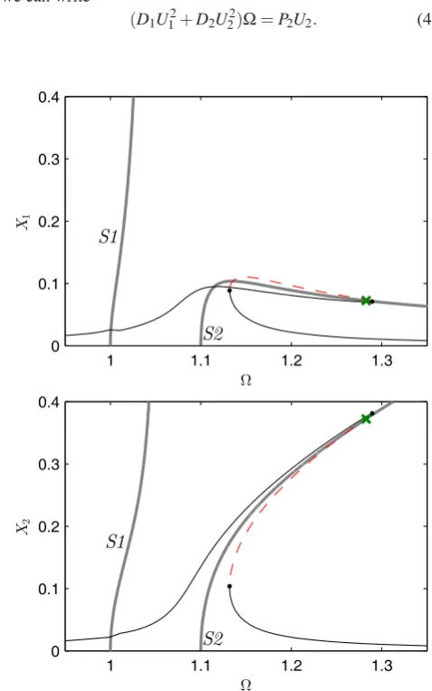
Figure 3. Backbone curves and forced response of the system whenκ=5 in the projection of response frequency,Ω, against displacement amplitude of the Þrst and second mass,X1andX2, in panels (a) and (b) respectively. Thick

grey lines represent the backbone curves and the forced response is shown as thin black lines and dashed red lines for the stable and unstable branches respectively. Green crosses represent the crossing points predicted by energy balancing and the fold points on the forced response are represented by black dots.

Figure 3 shows the energy balancing technique applied to the example system, with the parameters given in Eq. (12) where κ=5. The backbone curves and the crossing points predicted by the energy balancing technique are compared to the forced response. It can be seen that, as expected, the forced response does not tend towardsS1, due to the lowq2component inS1.

Hence, no crossing point has been predicted here. The predicted crossing point onS2is good, although not precise. This is due to the fact that on the backbone curves, there is no net energy transfer between q1 and q2. However, as q1 is damped but

unforced, the forced response must be such that there is a net energyßow fromq2to q1. Therefore, the assumption that the

forced response crosses the backbone curves precisely cannot be true.

5 OPTIMISATION

As an example of how the technique may be used to optimise a system, consider the case where an energy harvesting device connects the second mass to ground. As this device acts like a damper, it does not affect the backbone curves but does affect the point at which the forced response crosses the backbone curves, as predicted by the energy balancing technique. Therefore, by varying the nonlinear parameter,κ, we can describe the change in the underlying behaviour using the backbone curves and the change in the forced response using the energy balancing technique. This approach can be used to optimise the system with respect toκ.

For this example, it is required that the maximum displace-ment of the Þrst mass, X1, must not exceed 0.125, whilst it

is desirable to maximise the potential of the system to harvest energy. As the basin of attraction of the upper branch decreases withΩ, we estimate the probability that the response will settle to the upper branch of the response, as

P(Ω) = ΩEB−Ω

(ΩEB−ωn2)

1000(Ω₋ωn2)2+1

, (48)

whereΩEBis the value ofΩat the crossing point determined by

the energy balancing.

5.1 FINDING THE MAXIMUM VALUE OF X1

From Figure 2 it can be seen that the maximum value of X1

occurs at the point wheredX1

dΩ =0. From Eqs. (40), this can be

found using

d dΩ

ω2 n2−ωn21

Ω2₋ω2 n1

U2(Ω) =0, (49a)

−2Ωω₂

n2−ωn21

_Ω2

−ωn21

2 U2(Ω) + ω2

n2−ωn21

Ω2_−ω2 n1

U₂′(Ω) =0, (49b) 2Ω

ωd1

U2(Ω) +U2′(Ω) =0, (49c)

where_•′_represents d•

dΩ and, from Eq. (32)

U2(Ω) =

$ 8m_Ω2

−ωn22

3κ

%1₂

ω2

n1−Ω2

ω2

n1+ωn22−2Ω2

32

, (50a)

= (A)12_(B)32_, (50b)

where

A=−8mωd2

3κ , B=

ωd1

ωd1+ωd2. (51)

From this, we can calculate

U₂′(Ω) =A12 d dΩ

B23

+B32 d

dΩ

A12

, (52a)

= 3 2A

1

2_B12_B′₊1 2A

−12_B32_A′_{, (52b)}

where A′= d dΩ

8mΩ2_−ω2 n2

3κ

, (53a)

= 16mΩ

3κ , (53b)

and B′= d

dΩ

ω2

n1−Ω2

ω2

n1+ωn22−2Ω2

, (53c)

= 2Ω(ωd1−ωd2) (ωd1+ωd2)2

. (53d)

Substituting Eqs. (53b) and (53d) into Eq. (52b) leads to

U₂′= (AB)12 $

3Ω(ωd1−ωd2)

(ωd1+ωd2)2

% +B

3 2

A12 _8mΩ

3κ

. (54)

Substituting Eqs. (50b) and (54) into Eq. (49c) and simplifying gives

ω2

d1+ωd22−4ωd1ωd2=0. (55)

This can then be written as a quadratic in Ω2_{, using Eq. (24),}

and solved to give

2Ω2=ω_n21+ωn22±

√

3ω2

n2−ωn21. (56)

AsΩmust be real, the positive root must be chosen, leading to

Ω= & ' ' ( $

1−√3 2

% ω2

n1+

$ 1+√3

2 %

ω2

n2, (57)

which shows that the frequency at which the maximum value of X1occurs is independent ofκ. Substituting this into Eqs. (39),

(32) and (24) it is found that the maximum value ofX1 on the

backbone curve is given by

X1,MAX=

"

4√3_ω2

n2−ωn21

m

27κ . (58)

ForX1to be less than 0.125, it is required

κ > 4

√

3ω2 n2−ωn21

m

27(0.125)2 , (59a) >3.45 (to 3 signiÞcantÞgures). (59b)

5.2 OPTIMISING FOR X2

With a minimum value for κ deÞned by Eqs. (59) we can now optimise the system with respect to its potential to harvest energy. The energy harvested from the device is proportional to the velocity ofx2, i.e. proportional toΩX2. Using Eq. (48),

we can deÞne the probabilistic energy harvesting capability at a givenΩ(whereΩ_∈[ωn2,ΩEB]) asP(Ω)ΩX2. Therefore, the

overall capability of the system in harvesting energy over all forcing frequencies is given by the proportional relation

EH∝

# ΩEB

ωn2

P(Ω)ΩX2dΩ, (60)

3.5 4 4.5 5 5.5 6 6.5 7

4_.64

κ EH

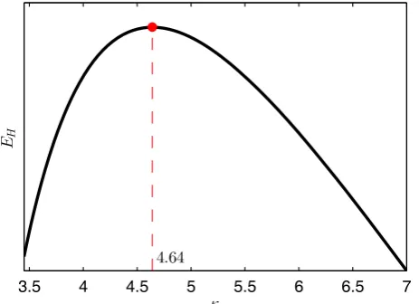
Figure 4. Nonlinear coefÞcient,κ, against proportional energy harvesting capability of the system. The red dot shows the point at which the energy harvesting capability is at its maximum.

This may be calculated for a range of values of κ, where κ>3.45 in keeping with Eq. (59b). Figure 4 showsκagainst proportional energy harvesting capability of the system. The point of maximum capability is represented by a red dot, and corresponds toκ=4.64. At this value the maximum value of X1is given byX1=0.1078, which is below the limit of 0.125.

6 CONCLUSION

This work shows how the second-order normal form technique can be used to develop analytical expressions describing the response of MDOF nonlinear systems. We have demonstrated that by describing the backbone curves of such systems we can interpret the underlying behaviour, independent of forcing and damping. This provides a simple method for determining the characteristics of nonlinear systems, and is well suited for use in the analysis of larger systems. Backbone curves also allow some features of the response of a system to be optimised independently of forcing and damping. This provides a simpliÞcation of the response along with a design tool for nonlinear systems where the forcing and damping characteristics are unknown.

The relationship between backbone curves and the forced response can be determined using the energy balancing tech-nique introduced here. This may allow further simpliÞcation of systems by disregarding backbone curves that are not followed under particular forcing and damping conditions. As the energy balancing technique is also analytical, it may be used alongside the analytical design and optimisation enabled by the second-order normal form technique. The accuracy may be further increased by accounting for the harmonic terms in both the backbone curves and the energy balancing technique, and by allowing for a higher order of accuracy in the second-order normal form technique.

The limitations of this approach are dictated by the need for the systems to be weakly nonlinear, in order for the second-order normal form technique to be valid. It is preferable that, when the system is forced, the energy transfer within the

system is small. This allows the forced response to approach the backbone curves, increasing the accuracy of the energy balancing technique.

REFERENCES

[1] E.J. Doedel, with major contributions from A.R. Champneys, T.F. Fairgrieve, Y.A. Kuznetsov, F. Dercole, B.E. Oldeman, R.C. Paffenroth,

B. Sandstede, X.J. Wang and C. Zhang, AUTO-07P: Continuation and

Bifurcation Software for Ordinary Differential Equations, Concordia

University, Montreal, Canada, (2008). http://cmvl.cs.concordia.ca . [2] G. Kerschen, M. Peeters, J.C. Golinval and A.F. Vakakis, Nonlinear normal

modes, Part I: A useful framework for the structural dynamicist,Mechanical

Systems and Signal Processing, 23, 170 - 194, (2009).

[3] M. Peeters, R. Vigui, G. Srandour, G. Kerschen and J.C. Golinval, Nonlinear normal modes, Part II: Toward a practical computation

using numerical continuation techniques,Mechanical Systems and Signal

Processing, 23, 195 - 216, (2009).

[4] A.H. Nayfeh and D.T. Mook,Nonlinear Oscillations, Wiley, (2008).

[5] R. Khanin, M. Cartmell and A, Gilbert, A computerised implementation of

the multiple scales perturbation method using Mathematica,Computers &

Structures, 76, 565-575, (2000).

[6] D.I.M. Forehand and M.P. Cartmell, The implementation of an automated method for solution term-tracking as a basis for symbolic computational

dynamics,Proceedings of the Institution of Mechanical Engineers, Part C:

Journal of Mechanical Engineering Science, 225, 40-49, (2011).

[7] J. Murdock,Normal Forms and Unfoldings for Local Dynamical Systems,

Springer, (2002).

[8] S.A. Neild, Approximate Methods for Analysing Nonlinear Structures,

Exploiting Nonlinear Behavior in Structural Dynamics, Springer, Vienna,

CISM Courses and Lectures, 53-109, (2012).

[9] S.A. Neild and D.J. Wagg, Applying the method of normal forms to

second-order nonlinear vibration problems,Proceedings of the Royal Society A:

Mathematical, Physical and Engineering Science, 467, 1141-1163, (2010).

[10] D.J. Wagg and S.A. Neild,Nonlinear Vibration with control,