Journal of Applied
Crystallography
ISSN 1600-5767
Received 1 August 2013 Accepted 30 October 2013
Global small-angle X-ray scattering data analysis
for multilamellar vesicles: the evolution of the
scattering density profile model
Peter Heftberger,aBenjamin Kollmitzer,aFrederick A. Heberle,b Jianjun Pan,b,c Michael Rappolt,d,eHeinz Amenitsch,dNorbert Kucˇerka,fJohn Katsarasb,g,h,iand Georg Pabsta*
a
Instiute of Molecular Biosciences, Biophysics Division, University of Graz, Austria,bBiology and Soft Matter Division, Oak Ridge National Laboratory, Oak Ridge, TN, USA,cDepartment of Physics, University of South Florida, Tampa, FL 33620, USA,dInstitute of Inorganic Chemistry, Graz University of Technology, Austria,eSchool of Food Science and Nutrition, University of Leeds, UK, f
Canadian Neutron Beam Centre, National Research Council, Chalk River, ON, Canada,gJoint Institute for Neutron Sciences, Oak Ridge, TN, USA,hDepartment of Physics and Astronomy, University of Tennessee, Knoxville, TN, USA, andiDepartment of Physics, Brock University, St Catharines, ON, Canada. Correspondence e-mail: [email protected]
The highly successful scattering density profile (SDP) model, used to jointly analyze small-angle X-ray and neutron scattering data from unilamellar vesicles, has been adapted for use with data from fully hydrated, liquid crystalline multilamellar vesicles (MLVs). Using a genetic algorithm, this new method is capable of providing high-resolution structural information, as well as determining bilayer elastic bending fluctuations from standalone X-ray data. Structural parameters such as bilayer thickness and area per lipid were determined for a series of saturated and unsaturated lipids, as well as binary mixtures with cholesterol. The results are in good agreement with previously reported SDP data, which used both neutron and X-ray data. The inclusion of deuterated and non-deuterated MLV neutron data in the analysis improved the lipid backbone information but did not improve, within experimental error, the structural data regarding bilayer thickness and area per lipid.
1. Introduction
Phospholipids are a major component of biological membranes, and the structural analysis of pure lipid membranes is an important area of research, as it can provide valuable insights into membrane function, including how the membrane’s mechanical properties affect lipid/protein inter-actions (Escriba´et al., 2008; Mouritsen, 2005). Of the liquid crystalline mesophases formed by phospholipids in aqueous solutions, most effort has been expended in studying fluid bilayers (L), because of their commonly accepted biological
significance.
Over the years, scattering techniques such as small-angle X-ray and neutron scattering (SAXS and SANS) have been widely used to determine the structural parameters and mechanical properties of biomimetic membranes. With regard to bilayer structure, two important structural parameters are bilayer thickness and lateral area per lipidA(Lee, 2004; Pabst
et al., 2010; Heberleet al., 2012); the latter is directly related to lipid volume and inversely proportional to bilayer thickness. Importantly,Aplays a key role in the validation of molecular dynamics (MD) simulations (Klaudaet al., 2006), and as such, its value for different lipids must be accurately known.
Historically, for a given lipid, a range of values for A have been reported (Kucˇerkaet al., 2007). Since lipid volumes are determined from independent and highly accurate densito-metry measurements (Nagle & Tristram-Nagle, 2000; Green-woodet al., 2006; Uhrı´kova´et al., 2007), differences inAmust therefore result from differences in bilayer thickness. To accurately determine lipid areas, a precise measure of the Luzzati thicknessdB(Luzzati & Husson, 1962), which is given
by the Gibbs dividing surface of the water/bilayer interface (Kucˇerka, Nagleet al., 2008), is needed. Other frequently used definitions of bilayer thickness are the headgroup-to-head-group thicknessdHH and the steric bilayer thickness (Pabst,
Katsaraet al., 2003). The latter two bilayer thicknesses can also be used to determineA; however, assumptions regarding the headgroup size or the distance to the chain/headgroup interface have to be made.
phosphate group, which is part of the phosphorylcholine headgroup, and hence accurate values for dHH can be
obtained. On the other hand, neutrons are scattered by atomic nuclei and can be used for contrast variation analyses, since hydrogen and its isotope deuterium scatter neutrons with similar efficiencies but 180out-of-phase with each other (i.e.
deuterium’s coherent scattering length is positive, while hydrogen’s is negative). In the case of protiated lipid bilayers, SANS is highly sensitive to locating the hydrogen-depleted carbonyl groups. Importantly, however, neutron contrast can be easily tuned by varying the hydrogen–deuterium content of the water (by varying the H2O/D2O ratio) or of the bilayer
(through the use of deuterated lipids) (Pabstet al., 2010). As mentioned, in the case of protiated lipid bilayers in 100% D2O, neutrons are most sensitive to the lipid’s glycerol
backbone. Moreover, the Gibbs dividing surface for the apolar/polar interface is typically located between the head-group phosphate and the lipid backbone. Therefore a combined analysis of X-ray and neutron data should yield the most accurate values ofdBandA(Kucˇerka, Nagleet al., 2008;
Kucˇerka et al., 2011; Pan, Heberle et al., 2012). In this combined data analysis, commonly known as the scattering density profile (SDP) model, the lipid bilayer is represented by volume distributions of quasi-molecular fragments, which are easily converted into electron density or neutron scattering length density distributions by scaling them (for a given molecular group) with the appropriate electron or neutron scattering length density [see Heberleet al.(2012) for a recent review].
Scattering techniques are also capable of probing membrane elasticity. Lipid bilayers are two-dimensional fluids which exhibit significant bending fluctuations of entropic origin. In multilamellar arrangements,e.g.in liquid crystalline multilamellar vesicles (MLVs) or surface-supported multi-bilayers, this leads to a characteristic power-law decay of the positional correlation function, known as quasi-long-range order, with Bragg peaks having characteristic line shapes (Liu & Nagle, 2004; Salditt, 2005; Pabst et al., 2010). Membrane elasticity can therefore be determined from line-shape analysis of the Bragg peaks, and the underlying physics of this phenomenon is described by the Caille´ (1972) or modified Caille´ theory (MCT) (Zhanget al., 1994). The resulting fluc-tuation, or Caille´ parameter , is a function of the bilayer bending modulus and the bulk modulus of interbilayer compression. Owing to the higher-resolution data, compared to neutrons, X-rays are better suited for line-shape analysis of Bragg peaks.
Just over a decade ago, Pabst and co-workers were the first to report a full-q-range analysis of MLV SAXS data using MCT (Pabstet al., 2000; Pabst, Koschuchet al., 2003). In that method, quasi-Bragg peaks and diffuse scattering were both taken into account when analyzing the data, and the electron density profile was modeled by a simple summation of Gaussians representing the electron-rich lipid headgroup and electron-poor (in relation to the headgroup) hydrocarbon
The work described here extends the global analysis program (GAP; Pabstet al., 2000; Pabst, Koschuchet al., 2003) for MLVs, by making use of the SDP description of the lipid bilayer. This modified technique, termed herein the SDP– GAP model, has several advantages. Firstly, compared to extruded unilamellar vesicles (ULVs), spontaneously forming MLVs are easier to prepare (Heberleet al., 2012). Secondly, the SDP description of the bilayer imparts to GAP the ability to simultaneously analyze SANS and SAXS data, while enabling the SDP model to determine bending fluctuations and, hence, bilayer interactions.
In the present study we also attempted to determine precise values ofdBandAusing standalone X-ray data. Such analysis,
however, is complicated by the use of an increased number of fitting parameters, as compared to GAP, and inherently less scattering contrast, as compared to the SDP model, which simultaneously makes use of SANS and SAXS data. To address these shortcomings we used a genetic algorithm, as an optimization routine, in combination with information from other sources, thereby reducing the number of parameters needed by the SDP–GAP model. To test the new SDP–GAP model, we analyzed a series of saturated and unsaturated phospholipids, as well as binary lipid mixtures with choles-terol. The results compare favorably with previously reported data obtained using the SDP model, including the commonly accepted bilayer condensation effect induced by cholesterol. We also include SANS data of protiated and deuterated palmitoyl-oleoyl phosphatidylcholine (POPC) in our analysis, which gives rise to a better resolved location of the lipid’s glycerol backbone. Compared to standalone SAXS analysis, any differences in the values ofAanddBobtained from
SDP-GAP model analysis are well within experimental uncertainty.
2. Material and methods
2.1. Sample preparation
1,2-Dipalmitoyl-sn-glycero-3-phosphocholine (DPPC), 1-pal-mitoyl-2-oleoyl-sn-glycero-3-phosphocholine (POPC), 1-palmit-oyl(d31)-2-oleoyl-sn-glycero-3-phosphocholine (POPC-d31), 1-stearoyl-2-oleoyl-sn-glycero-3-phosphocholine (SOPC) and 1,2-dioleoyl-sn-glycero-3-phosphocholine (DOPC) were purchased from Avanti Polar Lipids, Alabaster, AL, USA, and cholesterol was obtained from Sigma–Aldrich (Austria). 99.8% D2O was
obtained from Alfa Aesar (Ward Hill, MA, USA). All lipids were used without further purification.
For neutron experiments, MLVs of POPC-d31 at 10 mg ml1 were prepared by weighing 15 mg of dry lipid powder into 13100 mm glass culture tubes and hydrating with 1.50 ml D2O preheated to 313 K, followed by vigorous
vortexing to disperse the lipid. The resultant MLV suspension was incubated at 313 K for 1 h, with intermittent vortexing, and then subjected to five freeze/thaw cycles between 193 and 313 K to reduce the average number of lamellae and facilitate extrusion (Kaasgaardet al., 2003; Mayeret al., 1985). A 0.75 ml aliquot of the MLV sample was used to prepare ULVs using a hand-held miniextruder (Avanti Polar Lipids, Alabaster, AL, USA) assembled with a 50 nm-pore-diameter polycarbonate filter and heated to 313 K. The suspension was passed through the filter 41 times. ULV samples were measured within 24 h of extrusion. The final sample concentrations were 10 mg ml1, which allows for sufficient water between vesicles to eliminate the interparticle structure factor, thereby simplifying data analysis.
2.2. Small-angle X-ray scattering
X-ray scattering data were acquired at the Austrian SAXS beamline, which is situated at the Elettra synchrotron (Trieste, Italy), using 8 keV photons. Diffraction profiles were detected utilizing a Mar300 image-plate detector (Marresearch GmbH, Norderstedt, Germany) and calibrated using a powder sample of silver behenate. Lipid dispersions were taken up in 1 mm-thick quartz capillaries and inserted into a multi-position sample holder. Samples were equilibrated for a minimum of 10 min prior to measurement at a predetermined temperature with an uncertainty of0:1 K using a circulating water bath. The exposure time was set to 240 s. Scattering patterns were integrated using the program FIT2D (Hammersley, 1997). Background scattering originating from water and air was subtracted, and data sets were normalized using the trans-mitted intensity, which was measured by a photodiode placed in the beamstop.
2.3. Small-angle neutron scattering
Neutron scattering experiments were performed using the Extended-Q-range Small-Angle Neutron Scattering (EQ-SANS, BL-6) instrument at the Spallation Neutron Source (SNS) located at Oak Ridge National Laboratory (ORNL). ULVs were loaded into 2 mm-path-length quartz banjo cells (Hellma USA, Plainview, NY, USA) and mounted in a temperature-controlled cell paddle with a 1 K accuracy. In 60 Hz operation mode, a 4 m sample-to-detector distance with a 2.5–6.1 A˚ wavelength band was used to obtain the relevant wavevector transfer. Scattered neutrons were collected with a two-dimensional (11 m) 3He position-sensitive detector
made up of 192256 pixels. Two-dimensional data were reduced using MantidPlot (http://www.mantidproject.org/). During data reduction, the measured scattering intensity was corrected for detector pixel sensitivity, dark current, sample transmission, and background scattering contribution from the water and empty cell. The one-dimensional scattering
intensity,I versus q, was obtained by radial averaging of the corrected two-dimensional data.
2.4. Modeling of phospholipid bilayer
To analyze the scattering profile of MLVs, we adopted the full-q-range GAP model of Pabst and co-workers (Pabstet al., 2000; Pabst, Koschuchet al., 2003), which takes into account diffuse scatteringNdifforiginating from positionally
uncorre-lated bilayers):
IðqÞ ¼ ð1=q2Þ FðqÞ2SðqÞð1N
diffÞ þ FðqÞ 2
Ndiff
h i
; ð1Þ
where the scattering vector magnitudeq¼4sin=,is the wavelength, 2is the scattering angle relative to the incident beam, FðqÞ is the bilayer form factor and SðqÞ is the inter-bilayer structure factor. For fluid lipid inter-bilayers,SðqÞis given by the Caille´ theory, which is described in detail elsewhere (Caille´, 1972; Zhang et al., 1994; Pabst et al., 2000; Pabst, Koschuchet al., 2003). Averaging over variations in scattering domain size was performed following Fru¨hwirthet al.(2004). One of the important parameters determined from fittingSðqÞ
using MCT is the Caille´ parameter, which is a measure of bending fluctuations (Pabst et al., 2010). The number of positionally correlated bilayersNmean affects the width of the
Bragg peaks (Pabst, Koschuchet al., 2003) and must be opti-mized through fitting of the data. In the case of the present samples, the number of bilayersNmean contributing to Bragg
scattering varied between ten and 30. Instrumental resolution was taken into account by convoluting equation (1) with the beam profile (Pabst et al., 2000; Qian & Heller, 2011), and incoherent background scattering was accounted for by an additive constant.
The form factor is the Fourier transform of the electron density or neutron scattering length density profile. In the present study, we implemented the SDP model (Kucˇerka, Nagle et al., 2008) to describe the bilayer. The SDP model describes the membrane in terms of the volume distributions of quasi-molecular fragments. A detailed description of volume probability distribution functions is given in the article by Kucˇerka, Nagle et al. (2008). The water-subtracted scat-tering length density distributions [ðzÞ] are calculated by scaling the volume probability distributions using component total electron densities (for X-rays) or neutron scattering length densities. The form factor is then calculated as
FðqÞ ¼RðzÞexpðiqzÞdz: ð2Þ
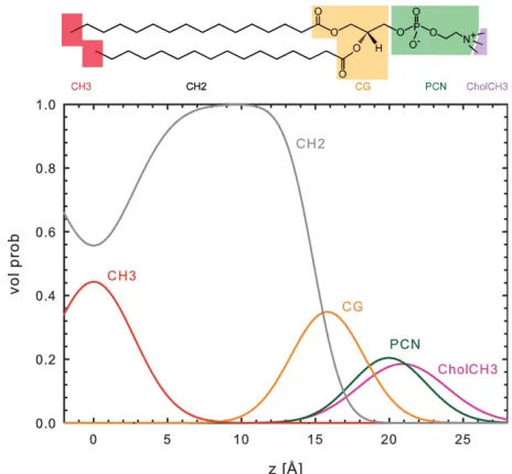
Kucˇerka and co-workers originally parsed phosphatidylcho-lines into the following components: choline methyl (CholCH3); phosphate + CH2CH2N (PCN); carbonyl +
glycerol (CG); hydrocarbon methylene (CH2); and
hydro-carbon terminal methyl (CH3). An additional methine (CH)
group was added for unsaturated hydrocarbon chains. However, the contrast between CH and CH2is weak, even for
To avoid nonphysical results, the following constraints were adopted following Klauda et al. (2006) and Kucˇerka, Nagle
et al.(2008). Because of bilayer symmetry, the position of the terminal methyl groupzCH3was set to zero and the height of
the error function, which describes the hydrocarbon chains, was set to one in order to comply with spatial conservation. The width of the choline methyl groupCholCH3 was fixed to
2.98 A˚ , and the width of the error function describing the hydrocarbon chain was constrained within accepted limits (HC2 ½2:4;2:6A˚ ) (Klaudaet al., 2006; Kucˇerka, Nagleet al.,
2008).
We also implemented new constraints to aid the standalone X-ray data analysis. Firstly, the distances between the CholCH3and PCN groups, and the hydrocarbon chain
inter-face (zHC) and CG (zCG) groups, were not allowed to exceed
2 A˚ because of their spatial proximity. Secondly, volumes of the quasi-molecular fragments, necessary for calculating electron or neutron scattering length densities, were taken from previous reports (Kucˇerka et al., 2005, 2011; Kucˇerka, Nagleet al., 2008; Klaudaet al., 2006; Greenwoodet al., 2006) and allowed to vary by 20%. The total volume of the headgroup components (i.e. CholCH3, PCN and CG) was
constrained to a target value of 331 A˚3, as reported by
Tris-tram-Nagle et al. (2002), whereby the value is allowed to deviate from the target value, but in doing so, incurs a good-ness-of-fit penalty.
For lipid mixtures with cholesterol, cholesterol’s volume distribution was merged with that of the CH2group, following
Pan, Cheng et al. (2012). This is justified on the basis of cholesterol’s strong hydrophobic tendency, which dictates its location within the hydrocarbon chain region, and the fact that its hydroxy group resides in the vicinity of the apolar/polar interface (Pan, Chenget al., 2012). In calculating the lipid area for binary mixtures, the apparent area per lipidA¼2VL=dB
was used (Pan, Chenget al., 2012; Panet al., 2009). The volume of cholesterol within lipid bilayers was taken to be 630 A˚3 (Greenwoodet al., 2006).
2.5. Determination of structural parameters
On the basis of volume probability distributions and scat-tering length density profiles, membrane structural parameters were defined as follows: (i) the headgroup-to-headgroup distance dHH is the distance between maxima of the total
electron density (i.e.the sum of the component distributions); (ii) the hydrocarbon chain lengthdCis the position of the error
function representing the hydrocarbon region zHC; and (iii)
the Luzzati thickness dB is calculated from the integrated
water probability distribution (Kucˇerka, Nagleet al., 2008):
dB¼d2
R
d=2
0
PWðzÞdz; ð3Þ
wheredis the lamellar repeat distance. The volume distribu-tion funcdistribu-tion of water was previously defined as (Kucˇerka, Nagleet al., 2008)
PWðzÞ ¼1
P
PiðzÞ; ð4Þ
where i indexes the lipid component groups (i.e. CholCH3,
PCN, CG, CH2and CH3). In order to increase the robustness
of the analysis fordB,PWobtained from the SDP analysis was
fitted with an error function, thus giving greater weight to the region close to the lipid headgroup (owing to the higher X-ray contrast) compared to the hydrocarbon chain region. We also attempted to include thePW model function in the SDP fit;
however, the results were not satisfactory. The area per lipid is then given by (Kucˇerka, Nagleet al., 2008)
A¼2VL=dB; ð5Þ
whereVL is the molecular lipid volume determined by
sepa-rate experiments. Finally, the thickness of the water layer was defined as
dW¼ddB: ð6Þ
2.6. Fitting procedure
Owing to the large number of adjustable parameters (i.e.
21) and our goal to apply the SDP–GAP model to standalone X-ray data, we chose to use a genetic algorithm in the opti-mization routine. The main benefit of this algorithm, compared to simple gradient descent routines or more sophisticated optimization algorithms (e.g. Levenberg– Marquardt), is that the fitting procedure does not easily fall into local minima (Goldberg, 1989). Briefly, a random set of adjustable parameters (termed a population) is chosen within fixed boundaries and tested for its fitness, defined here as the reduced chi squared ( 2) value, which is equal to the sum of the squared residuals divided by the degrees of freedom (Press
et al., 2007). The best solutions are then combined to obtain a new and better population, in a manner similar to the
[image:4.610.54.286.494.709.2]tions of2000 individuals were tested for their fitness. If 2
does not change after 100 generations, the optimization is assumed to have converged and the routine is terminated. Solutions with the lowest 2 values are then compared with
respect to differences in structural parameters. From the resulting distributions we estimate that the uncertainty of all parameters reported in the present work is 2%. Applica-tion of genetic algorithms comes with a greater computaApplica-tional cost, and they are most efficient when using parallel processing techniques. For the present study, all routines were encoded in IDL (Interactive Data Language), using the SOLBER opti-mization routine (Rajpaul, 2012). Typical runtimes for one X-ray scattering profile were between three and five hours on a six core machine (Intel Xeon 2.67 GHz).
3. Results and discussion
3.1. X-ray standalone data
The SDP–GAP model was tested on SAXS data obtained from single component Llipid bilayers and selected binary
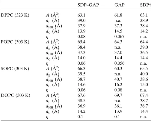
mixtures of phosphatidylcholines with cholesterol. As an example of our analysis, we present results for SOPC bilayers with five lamellar diffraction orders (Fig. 2). Fits from all other bilayers, including tables with structural parameters, are given in the supporting material (Figs. S1–S3, Table S1).1All SAXS patterns showed significant diffuse scattering, originating from membrane fluctuations common toLbilayers. In particular,
bending fluctuations lead to a rapid decrease in diffraction peak amplitudes as a function of q, and quasi-Bragg peaks with characteristic line shapes. Such effects are accounted for in the structure factor used. We found good agreement between the SDP–GAP model and experimental SOPC data ( 2¼0:78). Fits from other MLV systems yielded similar 2 values (Table S1). Omitting the constraints introduced inx2.4 led to slightly improved 2values but produced nonphysical
results.
Results from the SDP–GAP model were compared with those from the GAP model. The GAP data were in reasonable agreement with the experimental data (Fig. 2), albeit with poorer fit statistics ( 2¼4:78), which could be attributed to
[image:5.610.313.565.116.319.2]the small deviations of the model between the various Bragg peaks. Despite the good fits produced using the GAP model, the structural features obtained from SDP–GAP analysis are significantly richer (Fig. 2, lower panel). This point is illu-strated by the total electron density shown in the inset to Fig. 2, where the methyl trough is smeared out in the GAP electron density profile.
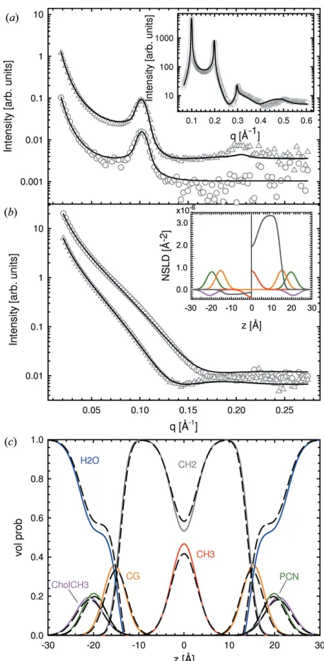
Table 1 provides the main structural parameters obtained from SDP–GAP and GAP analyses of the same data, as well as literature values obtained from SDP analysis (i.e. joint
Figure 2
[image:5.610.48.294.329.679.2]SDP–GAP analysis of SOPC MLVs at 303 K. Panel (a) compares the SDP–GAP (black line) and GAP models (red dashed line) with experimental data (grey circles). The inset to the figure compares the corresponding electron density profiles. Panel (b) shows the volume probability distribution (left hand side) and the electron density distributions of the defined quasi-molecular fragments (right hand side).
Table 1
Comparison of structural parameters.
Parameter uncertainties are estimated to be<2% as described inMaterials and methods.
SDP–GAP GAP SDP†
DPPC (323 K) A(A˚2) 63.1 61.8 63.1
dB(A˚ ) 39.0 n.a. 38.9
dHH(A˚ ) 37.9 37.3 38.4
dC(A˚ ) 13.9 14.5 14.2
0.08 0.067 n.a.
POPC (303 K) A(A˚2) 65.4 64.3 64.4
dB(A˚ ) 38.4 n.a. 39.0
dHH(A˚ ) 37.3 37.0 36.5
dC(A˚ ) 14.0 14.4 14.4
0.06 0.056 n.a.
SOPC (303 K) A(A˚2) 66.3 60.3 65.5
dB(A˚ ) 39.5 n.a. 40.0
dHH(A˚ ) 38.7 40.7 38.6
dC(A˚ ) 14.6 16.2 15.0
0.06 0.08 n.a.
DOPC (303 K) A(A˚2) 67.6 69.7 67.4
dB(A˚ ) 38.5 n.a. 38.7
dHH(A˚ ) 36.9 36.1 36.7
dC(A˚ ) 14.2 13.9 14.4
0.1 0.1 n.a.
† From Kucˇerka, Nagleet al.(2008) and Kucˇerkaet al.(2011).
1
refinement of SAXS and SANS data). The calculation of structural parameters using the GAP model is detailed by Pabst, Katsaraset al.(2003). Our results using the SDP–GAP model are in good quantitative agreement with the reference data. Deviations from the GAP model are, however, larger (though still reasonable) because of the simplified electron density model that was used. Interestingly, in the case of some lipids, we also find significant differences for the fluctuation parameter; these are attributable to the form factor, which modulates peak intensity. It therefore stands to reason that the better fits to the experimental data by the SDP–GAP model should result in more accuratevalues.
We further tested the SDP–GAP model using the same lipid systems, but this time with the addition of 20 mol% choles-terol. Cholesterol is abundant in mammalian plasma membranes and is well known for the condensing effect it has on lipid bilayers, which at the molecular level is explained by the umbrella model (Huang & Feigenson, 1999). In scattering studies, this effect shows up as an increase in dB and a
concomitant decrease in A, as well as in reduced bending fluctuations (seee.g.Hodzicet al., 2008). Fig. 3 shows the fits to SOPC/cholesterol membrane data. The SDP–GAP model is able to describe the better resolved higher diffraction orders
resulting from the presence of cholesterol. Our results show that cholesterol shifts the PCN and CholCH3groups further
away from the bilayer center (Fig. 3, bottom panel, and Tables 2 and S2), in good agreement with previous reports (Pan, Chenget al., 2012). On the other hand, we could not observe a significant shift of the CG group from the bilayer center or a higher value for the hydrocarbon chain thickness (Tables 2 and S2).
Structural parameters for all lipid mixtures are reported in Table 2. In agreement with previous reports, the addition of cholesterol causesAto decrease anddBanddHH to increase
(Hunget al., 2007; Kucˇerka, Perlmutteret al., 2008; Panet al., 2008; Hodzicet al., 2008; Pan, Chenget al., 2012). Compared to other membrane systems, bending fluctuations in DPPC bilayers experience a greater degree of damping when cholesterol is introduced, in agreement with the notion that cholesterol preferentially associates with saturated hydro-carbon chains (Panet al., 2009, 2008; Ohvo-Rekila¨et al., 2002). This effect is smaller for lipids having one monounsaturated chain (i.e.SOPC and POPC) and is completely absent when a second monounsaturated chain is introduced (e.g. DOPC). This latter finding is in good agreement with studies that reported no change in the bending rigidity of DOPC bilayers in the absence or presence of cholesterol (Panet al., 2008).
SOPC/cholesterol mixtures were also analyzed with the GAP model. Although reasonable fits are obtained (Fig. 3,
2
SDPGAP¼1:04, 2
GAP¼3:93), the differences in structural
parameters when comparing GAP data with SDP–GAP data are more pronounced. For example, the total electron density profiles show clear deviations in the acyl chain and headgroup regions. Cholesterol increases the asymmetry of the electron density distribution in the headgroup region, as determined from the SDP–GAP model, an effect that is not captured by the single-headgroup Gaussian of the GAP model. As a result, parameters such as area per lipid (ASDPGAP¼60:7 A˚
2
,
AGAP¼57:4 A˚ 2
) and hydrocarbon chain length (dC;SDPGAP¼
14.9 A˚ , dC;GAP¼17 A˚ ) differ between the two methods,
whereas the values for headgroup-to-headgroup thickness (dHH;SDPGAP¼42:1 A˚ , dHH;GAP¼42:3 A˚ ) and the Caille´
parameter (SDPGAP¼0:05, GAP¼0:04) are in reasonably
good agreement.
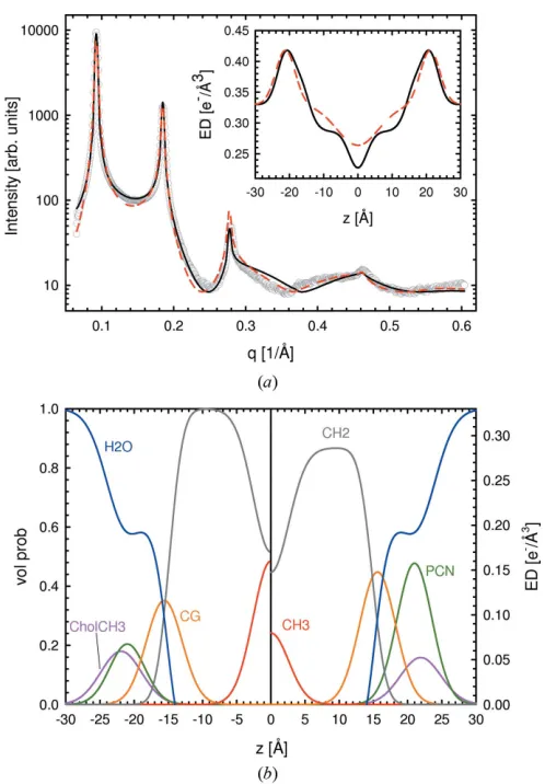
[image:6.610.314.565.125.185.2]3.2. Addition of SANS data
Figure 3
Table 2
Structural parameters from the SDP–GAP model of lipid bilayers containing 20 mol% cholesterol.
Parameter uncertainties are estimated to be<2% as described inMaterials and methods.
Lipid A(A˚2) dB(A˚ ) dHH(A˚ ) dC(A˚ )
DPPC (323 K) 61.2 40.1 42.3 14.2 0.02
POPC (303 K) 63.1 39.8 40.3 14.3 0.05
SOPC (303 K) 60.6 40.5 42.1 (42.1)† 14.9 (16.1)† 0.05
DOPC (303 K) 66.2 39.4 40.9 (39.0)† 13.5 (14.6)† 0.14
[image:6.610.47.296.353.711.2]information substantially alters the results. The protocol devised by Kucˇerka and co-workers used SANS data from protiated bilayers at different H2O/D2O contrasts (Kucˇerka,
Nagleet al., 2008).
Replacing H with D shifts the neutron scattering length density (NSLD) profile of the hydrocarbon region from negative to positive values (Fig. 4b, inset). Hence, relative to
D2O with an SLD = 6:410
14cm A˚3
, the hydrocarbon chain region contrast is significantly altered. This change in contrast manifested itself by producing two additional Bragg peaks in the case of POPC-d31 MLVs, compared to their protiated counterparts (Fig. 4a). Similarly, ULV data show a shift of the minimum at lowqto higherqvector magnitudes for POPC compared to POPC-d31 (Fig. 4b), which is also attributed to the change in contrast of the deuterated lipids in D2O.
We used SDP–GAP to simultaneously analyze SAXS data in several combinations with SANS data: (i) protiated MLVs; (ii) deuterated MLVs; and (iii) all four SANS data sets (i.e.
deuterated and protiated MLVs and ULVs). We also fitted all MLV data sets simultaneously and all ULV data sets sepa-rately. Fit results are shown in Fig. 4 and the determined structural parameters are summarized in Tables 3 and S3. The addition of a single SANS data set produced variations in the structural parameters, causing them to deviate from values determined from standalone SAXS analysis and those from the literature. This disagreement was rectified by including either both MLV data sets or all MLV and ULV data sets in the analysis. In the latter case, significant differences, compared to the standalone SAXS analysis, are found regarding the posi-tions of the CG group,zCGanddC. This can be understood in
terms of the better neutron contrast of the lipid backbone. Changes in volume distribution functions are shown in Fig. 4(c). The changes to A and dB are within the experimental
error and consequently of no significance. We thus conclude that the addition of SANS data helps to improve the location of the CG group and dC, but offers little improvement to
values ofAanddB.
4. Conclusion
We have modified the full-q-range SAXS data analysis, which previously used a simplified electron density profile (Pabst
[image:7.610.313.566.126.196.2]et al., 2000), with a high-resolution representation of scattering density profiles, based on volume distributions of quasi-molecular fragments (Kucˇerka, Nagleet al., 2008). The new SDP–GAP method, as its name implies, is a hybrid model that combines advantages offered by the GAP and SDP models. The SDP–GAP model can be used to analyze MLV and ULV data and is capable of simultaneously analyzing SAXS and
Figure 4
[image:7.610.55.284.167.634.2]Results of simultaneous SAXS and SANS analysis of data from POPC ULVs and MLVs at 303 K. Panel (a) shows SANS data of POPC (circles) and POPC-d31 (triangles) MLVs, and corresponding data obtained from ULVs (same symbols) are shown in panel (b). Solid lines are best fits to the data using the SDP–GAP model. The insets in panels (a) and (b) show the corresponding SAXS fits and neutron scattering length density profiles for POPC (left) and POPC-d31 (right), respectively. Panel (c) shows the changes in volume distributions from a SAXS-only analysis (dashed black lines) to a simultaneous SAXS/SANS analysis (colored lines; same color coding as in Figs. 2 and 3).
Table 3
Structural parameters for POPC using different combinations of SAXS and SANS data.
Parameter uncertainties are estimated to be<2% as described inMaterials and methods.
SAXS† n-MLVu‡ n-MLVd§ All data} SDP††
A(A˚2) 65.4 64.9 63.1 63.6 64.4
dB(A˚ ) 38.4 38.7 39.8 39.5 39.0
dHH(A˚ ) 37.3 37.1 37.3 37.5 36.5
dC(A˚ ) 14.0 14.6 14.4 14.3 14.4
zCG(A˚ ) 15.0 15.3 15.4 15.3 15.3
SANS data. MLVs are spontaneously formed membrane systems, and the development of this new hybrid model opens up new opportunities for the study of their bilayer interactions and membrane mechanical properties (e.g. elasticity) (Pabst
et al., 2010).
An additional feature of this new model is its ability to obtain high-resolution structural information from standalone SAXS data. This is achieved by implementing an optimization routine based on a genetic algorithm, which is able to deal with the large number of adjustable parameters, even though additional constraints and input parameters are required in order to limit parameter space. Compared to the GAP and SDP models, which use Levenberg–Marquardt and downhill simplex optimization routines, respectively, the computational effort required by the SDP–GAP model is significantly higher. Typical CPU times on parallel processors are of the order of a few hours, as compared to a few minutes for SDP or GAP. However, an advantage is that the genetic algorithm prevents the optimization routine from stalling in local minima. By using different seeds for the random number generator, robust results with good convergence are readily obtained
We have tested the SDP–GAP model using different satu-rated and unsatusatu-rated phosphatidylcholine bilayers, with and without cholesterol. Results fordBandAare in good
agree-ment with previous reports using the SDP model, although we note that the position and width of the CG group are subject to greater variabilities, as a result of the lower X-ray contrast of this particular group. This inadequacy was, however, ameliorated by including ULV SANS data. MLV SAXS data combined with ULV SANS data of POPC and POPC-d31 bilayers improved both the position of the CG group and the hydrocarbon chain thickness (Fig. 3cand Table 3). However, the values ofAanddBremained practically unchanged.
This work was supported by the Austrian Science Fund FWF, project No. P24459-B20 (to GP). Support was received from the Laboratory Directed Research and Development Program of Oak Ridge National Laboratory (to JK), managed by UT-Battelle, LLC, for the US Department of Energy (DOE). This work acknowledges additional support from the Scientific User Facilities Division of the DOE Office of Basic Energy Sciences, for the EQ-SANS instrument at the ORNL Spallation Neutron Source. This facility is managed for the DOE by UT-Battelle, LLC, under contract No. DE-AC05-00OR2275.
References
Caille´, A. (1972).C. R. Acad. Sci. Paris B,274, 891–893.
Escriba´, P. V., Gonza´lez-Ros, J. M., Gon˜i, F. M., Kinnunen, P. K., Vigh, L., Sa´nchez-Magraner, L., Ferna´ndez, A. M., Busquets, X., Horva´th, I. & Barcelo´-Coblijn, G. (2008).J. Cell. Mol. Med. 12, 829–875.
Fru¨hwirth, T., Fritz, G., Freiberger, N. & Glatter, O. (2004).J. Appl. Cryst.37, 703–710.
Goldberg, D. (1989).Genetic Algorithms in Search, Optimization, and
Greenwood, A. I., Tristram-Nagle, S. & Nagle, J. F. (2006).Chem. Phys. Lipids,143, 1–10.
Hammersley, A. (1997). FIT2D. Internal Report ESRF97HA02T. European Synchrotron Radiation Facility, Grenoble, France. Heberle, F. A., Pan, J., Standaert, R. F., Drazba, P., Kucˇerka, N. &
Katsaras, J. (2012).Eur. Biophys. J.41, 875–890.
Hodzic, A., Rappolt, M., Amenitsch, H., Laggner, P. & Pabst, G. (2008).Biophys. J.94, 3935–3944.
Huang, J. & Feigenson, G. W. (1999).Biophys. J.76, 2142–2157. Hung, W. C., Lee, M. T., Chen, F. Y. & Huang, H. W. (2007).Biophys.
J.92, 3960–3967.
Kaasgaard, T., Mouritsen, O. G. & Jørgensen, K. (2003).Biochim. Biophys. Acta Biomembr.1615, 77–83.
Klauda, J. B., Kucerka, N., Brooks, B. R., Pastor, R. W. & Nagle, J. F. (2006).Biophys. J.90, 2796–2807.
Kucerka, N., Liu, Y., Chu, N., Petrache, H. I., Tristram-Nagle, S. & Nagle, J. F. (2005).Biophys. J.88, 2626–2637.
Kucˇerka, N., Nagle, J. F., Sachs, J. N., Feller, S. E., Pencer, J., Jackson, A. & Katsaras, J. (2008).Biophys. J.95, 2356–2367.
Kucˇerka, N., Nieh, M.-P. & Katsaras, J. (2011). Biochim. Biophys. Acta Biomembr.1808, 2761–2771.
Kucˇerka, N., Pencer, J., Nieh, M.-P. & Katsaras, J. (2007).Eur. Phys. J. E Soft Matter,23, 247–254.
Kucˇerka, N., Perlmutter, J. D., Pan, J., Tristram-Nagle, S., Katsaras, J. & Sachs, J. N. (2008).Biophys. J.95, 2792–2805.
Lee, A. G. (2004).Biochim. Biophys. Acta Biomembr.1666, 62–87. Liu, Y. & Nagle, J. F. (2004).Phys. Rev. E,69, 040901.
Luzzati, V. & Husson, F. (1962).J. Cell Biol.12, 207–219.
Mayer, L., Hope, M., Cullis, P. & Janoff, A. (1985).Biochim. Biophys. Acta Biomembr.817, 193–196.
Mouritsen, O. G. (2005).Life as a Matter of Fat: the Emerging Science of Lipidomics.Berlin: Springer-Verlag.
Nagle, J. F. & Tristram-Nagle, S. (2000). Biochim. Biophys. Acta Biomembr.1469, 159–195.
Ohvo-Rekila¨, H., Ramstedt, B., Leppima¨ki, P. & Slotte, J. P. (2002). Prog. Lipid Res.41, 66–97.
Pabst, G., Katsaras, J., Raghunathan, V. A. & Rappolt, M. (2003). Langmuir,19, 1716–1722.
Pabst, G., Koschuch, R., Pozo-Navas, B., Rappolt, M., Lohner, K. & Laggner, P. (2003).J. Appl. Cryst.36, 1378–1388.
Pabst, G., Kucerka, N., Nieh, M. P., Rheinsta¨dter, M. C. & Katsaras, J. (2010).Chem. Phys. Lipids,163, 460–479.
Pabst, G., Rappolt, M., Amenitsch, H. & Laggner, P. (2000).Phys. Rev. E,62, 4000–4009.
Pabst, G., Zweytick, D., Prassl, R. & Lohner, K. (2012).Eur. Biophys. J.41, 915–929.
Pan, J., Cheng, X., Heberle, F. A., Mostofian, B., Kucˇerka, N., Drazba, P. & Katsaras, J. (2012).J. Phys. Chem. B,116, 14829–14838. Pan, J., Heberle, F. A., Tristram-Nagle, S., Szymanski, M., Koepfinger,
M., Katsaras, J. & Kucˇerka, N. (2012). Biochim. Biophys. Acta Biomembr.1818, 2135–2148.
Pan, J., Mills, T. T., Tristram-Nagle, S. & Nagle, J. F. (2008).Phys. Rev. Lett.100, 198103.
Pan, J., Tristram-Nagle, S. & Nagle, J. F. (2009). Phys. Rev. E, 80, 021931.
Press, W. H., Teukolsky, S. A., Vetterling, W. A. & Flannery, B. P. (2007).Numerical Recipes: The Art of Scientific Computing, 3rd ed. Cambridge University Press.
Qian, S. & Heller, W. T. (2011).J. Phys. Chem. B,115, 9831–9837. Rajpaul, V. (2012).arXiv:1202.1643[astro-ph.IM].
Salditt, T. (2005).J. Phys. Condens. Matter,17, R287–R314. Tristram-Nagle, S., Liu, Y., Legleiter, J. & Nagle, J. F. (2002).Biophys.
J.83, 3324–3335.
Uhrı´kova´, D., Ryba´r, P., Hianik, T. & Balgavy´, P. (2007).Chem. Phys. Lipids,145, 97–105.