Household location and income: a spatial analysis for British cities

Household location and income: a spatial analysis for

British cities

David Cuberes and Jennifer Roberts

ISSN 1749-8368

SERPS no. 2015022

1

Household location and income:

a spatial analysis for British cities

David Cuberes

Clark University

d.cuberes@clarku.edu

Jennifer Roberts

University of Sheffield

j.r.roberts@sheffield.ac.uk

October 2015

Abstract

Using information on the exact location of urban households in Britain for the period 2009-2013 we explore the validity of standard urban land use models by estimating the extent to which distance of residence from the city centre is a function of income. This is the first study of its kind for British cities. After controlling for household characteristics and access to transport, as well as city and time effects, and taking account of both spatial and serial correlation, we find a strong positive association between household’s income and distance from the city centre. We also estimate the income elasticity of demand for land and find that this is not large enough to support the view that richer households locate further from the city centre mainly because they prefer larger dwellings. Finally, we find that while poorer households live closer to the city centre, they have experienced increasing real incomes over the period relative to those who live further away. This supports the view that cities in Britain attract poor people rather than generate poverty.

JEL classification: I32, R23

Keywords: urban poverty; cities; segregation by income

1

2

1. Introduction

The majority of the poor in Great Britain currently live in urban areas. Within cities there are

distinct spatial patterns to deprivation; for example our data reveals that, in the period

2009-2013, the average monthly real income of households living within 0 to 5 percentile

distance of the city’s Central Business District (CBD) was £1,399, significantly lower than for

our sample of all urban households (£1,557)2.

Why do poor households tend to live in the inner cities? Is household location in cities

determined mostly by income? Is it the case that British cities tend to make households

poorer? Or is it rather the case that cities are good locations for the poor because, for

example, they have better access to public services?

In this paper we use data from the UK Household Longitudinal study ("Understanding

Society") to study the relationship between household income and location of residence in

the nine largest British metropolitan areas (excluding London) over the period 2009 to

20133. The analyzed cities are Birmingham, Bristol, Glasgow, Manchester, Leeds, Liverpool,

Newcastle, Nottingham, and Sheffield. We deliberately exclude London from the study

because both its size and structure are very different from the rest of British cities.4 Within

these cities we locate the exact position of households via their grid reference, and then

calculate their distance from the CBD. To estimate our models we use the spatial panel

estimator of Hsiang (2010), which is based on the generalised method of moments (GMM)

estimator for spatial data proposed by Conley (1999), and extends this to account for serial

correlation in longitudinal data.

To our knowledge this is the first study that explores the relationship between household

location and income in Britain using an economic framework. In fact, it is one of the very

few papers that analyses this question in any other country except the US. Further, our

study is one of the few that employ individual level analysis, and this is enabled by use of

2

Average income figures quoted throughout this paper are mean monthly equivalised real net household income in 2012/2013 prices.

3 _{We refer to metropolitan areas and cities interchangeably in the paper.} 4

3

secure data on exact household location, which is rarely used in economic analyses. As well

as the theoretical importance of this topic for urban economics, our findings also inform the

policy debate on urban poverty in Britain.

The paper is structured as follows. In Section 2 we provide a brief review of the literature

that has studied the relationship between income and household location in cities, most of

them in the US. In Section 3 we sketch the theoretical model advanced in Glaeser et al

(2008) to explore different explanations of household location within a city. The data are

described in Section 4. The econometric method, main empirical results and robustness

checks are discussed in Section 5. Finally, Section 6 concludes the paper.

2. Literature Review

Glaeser et al. (2008) study the location of the urban poor in US cities. Their first main result

is that there is a disproportionately larger incidence of poverty near a city’s CBD than farther

away from it. One possible explanation for this pattern is provided by standard urban land

use models (Alonso, 1964; Mills, 1967; Muth, 1969). In these models, rich households wish

to consume higher amounts of land, i.e. they would like to locate in larger houses than

poorer ones and therefore choose to live where land is cheaper, i.e. further away from the

CBD. However, introducing time costs associated with commuting in the model leads to an

ambiguous effect of income on location choices, as shown in Beckman (1974), Hochman and

Ofek (1977), Henderson (1977) and Fujita (1989). This is the result of the fact that rich

households have to choose between the utility they obtain from living in a large dwelling far

away from the CBD and the income loss associated with the long commute to their home.

Becker (1965) shows that the prediction that rich households locate further away from the

CBD than poor ones holds only if the income elasticity of demand for land is greater than

one.

In their analysis, Glaeser et al (2008) estimate income elasticities of demand for land in US

cities between 0.1 and 0.5, and thus they conclude that the standard monocentric city

4

argument, based on the model by LeRoy and Sonstelie (1983), is that the poor choose to live

in the CBD because they have access to better public transportation than in the suburbs.

Glaeser et al's (2008) calibrated version of this model provides strong evidence in favour of

this hypothesis. However, a recent paper by Gutierrez-i-Puigarnau et al (2014) provides

results that contradict much of the previous (largely US based) literature; they show that for

Denmark, conditional on the workplace location, the income elasticity of commuting

distance is negative and in the order of -0.18. This result could be due to the demand for

amenities, which in European cities tend to be clustered in city centres (Brueckner et al

1999). However it could also be specific to Denmark and the result of the highly regulated

rental housing market there.

One important difference between our work and this previous literature on commuting is

that we study distance to the CBD, not to the workplace. While this may be seen as

restrictive, households that locate close to the CBD may do so for many reasons other than

being close to their workplace (for example the availability of public transportation and

better amenities). More importantly, in our sample 32% of the heads of household do not

work, and this mean figure ranges from 26% to 41% across our cities. Focussing on both

employed and not-employed households is an important distinction between our paper and

the previous literature on commuting, where, by definition, only working households are

considered.

A further explanation for the spatial distribution of incomes is put forward by Brueckner and

Rosenthal (2009) who argue that the rich may decide to live in or near the CBD because they

value new construction more than the poor, and this construction often takes place in the

CBD. 5 Ng (2008) builds a model in which heterogeneity in household’s valuation of

amenities determines their location. Persky (1990) tests how well three different urban

models explain the pattern of income inequality in Chicago’ suburbs and finds that the

model that emphasizes local status (Frank, 1985) is the one that fits the data the best.

5

5

In the UK, the relevant literature has largely focused on the spatial concentration of poverty

and deprivation without testing any specific theoretical model (Rae, 2009; Galster, 2005). As

in the US, this has also been a major policy concern and focus of the urban planning debate

in the UK (DETR, 2000), among other reasons because concentrations of deprivation have

negative externalities due to the existence of 'neighbourhood' effects (Galster et al., 2007).

As mentioned above, it is well documented that UK deprivation is overly concentrated in

cities (Rae, 2012). This remains true even after the recent gentrification of city centres

(Rosenthal and Ross, 2015) facilitated both by the construction boom in high-quality

apartments that has characterised cities like Bristol and Manchester, and to a lesser extent

the rest of the cities we study here, and the enormous growth in student numbers in cities

resulting from the expansion of higher education (Tallon and Bromley, 2004). However, a

recent report from the Smith Institute argues that the wealth gap between the inner and

outer parts of cities is narrowing, as poverty is growing fastest in the suburbs (Hunter,

2014). In order to shed light on this topic we do what no work has done to date, and

explore the relationship between household income and urban location6, in order to test

whether the theoretical models of urban economics outlined in the next section are useful

in a British context.

3. Theoretical Framework

In this section we present a simplified version of the models first developed by Alonso

(1964), Mills (1967), and Muth (1969).7 Consider a city where all the jobs and amenities are

located in the CBD. Households commute to the CBD to either work, consume goods and/or

services or enjoy amenities. For simplicity, let us assume the CBD is collapsed to a single

point at the city centre, and that the city has a dense network of radial roads. The city

contains two different types of households: the rich, with income y_R and the poor, with

incomey_P, where y_R y_P. The two household types have the same preferences over the

two consumption goods, which are housing (q) and a composite good (c), with the latter

6

Rae (2012) studies the location of deprivation disaggregated by 'travel-to-work-area' in London, Birmingham, Liverpool and Manchester but no theoretical models are tested and the focus is on deprivation rather than income per se.

7

6

representing any consumption good other than housing. The cost of commuting to work at

the CBD is increasing in the distance x from the CBD and it has two components: a

monetary cost t, which increases linearly with distance and is assumed to be the same for

the two groups, and a cost related to the opportunity cost of time. Assuming that an extra

mile of commuting distance reduces available work time by a fraction



have higher wages than the poor (w_Rw_P) then the foregone income is larger for richer households. 8 The household budget constraint for the rich is then given by

)

( _R

R R

R pq y x t w

c     and for the poor is given by c_P pq_P y_Px(tw_P). On a )

,

(q p diagram then the slope of the two price schedules are −𝑡+𝛿𝜔_𝑞 𝑅

𝑅 and

−𝑡+𝛿𝜔𝑃

𝑞𝑃 ,

respectively. At the same housing price p, the higher income of the rich implies that they consume more housing (qR qP), making the slope of the price schedule flatter for the rich

group at that point. However, since wages are also higher for the rich, it is unclear which of

the two slopes is larger. Essentially, the rich group faces the following trade-off: on the one

hand, they wish to enjoy a large dwelling and so they benefit from living far from the CBD,

where housing costs are lower. On the other hand, commuting is more expensive for them

than for the low-income group, because their opportunity cost of time is higher. Therefore,

the location of rich and poor households in the equilibrium of the model can be

characterized by two different patterns, depicted in Figure 1. In the plot on the left, the rich

outbid the poor in the suburbs and therefore they end up living further away from the CBD.

The opposite happens in the plot on the right. As stated above, Becker (1965) shows that

the first scenario holds if and only if the income elasticity of demand for land is greater than

one. Ultimately, this is an empirical question that we analyze in Section 5.

8

7

4. Data and descriptive statistics

We use data from the first four waves of Understanding Society (University of Essex, 2015).

Understanding Society is a longitudinal survey of around 40,000 households in the UK.

Interviews for the first wave took place in 2009/10, with subsequent waves in 2010/11,

2011/12 and 2012/13. The sample of households was designed to be representative of the

UK population in 2008. All adults in each household are interviewed (as well as children

aged 11 to 15) and the data contain rich information on the social and economic

circumstances of households. As well as basic geographic information, such as which

Government Office Region a household is located in and whether the area is classified as

urban and rural9, the Secure Data Service (SDS)10 also provide access to detailed

geographical location for each household via grid reference.11 The Easting and Northing pair

of coordinates that make up a grid reference provide the exact location for each household

to a 1 metre resolution.

Our analysis covers the nine largest British metropolitan areas (Birmingham, Bristol,

Glasgow, Manchester, Leeds, Liverpool, Newcastle, Nottingham, and Sheffield), excluding

London. Households in these metropolitan areas were selected by matching their grid

reference to the postcode area code12 via the National Statistics Postcode Directories, and

then selecting only those households that were classified to be in an urban area; thus for

example those households in, say, the Sheffield (S) postcode area that are deemed to be

rural are excluded from our sample13.

The Understanding Society data is constructed at the individual level; with all individuals in

each household being interviewed. We construct a panel dataset at the household level by

9

Urban and rural classifications are given by the National Statistics Rural and Urban Classification of Output Areas at www.ons.gov.uk/ons/guide-method/geography/products/area-classifications/index.html

10

Details on the Secure Data Service can be found at ukdataservice.ac.uk/use-data/secure-lab

11

The British National Grid is the common referencing format for all geographic data in Great Britain. A location is described using two coordinates (Easting, Northing) which give its distance East and North of the origin, a fixed point to the west of the Scilly Isles.

12

The UK uses a system of alphanumeric postcodes to identify postal delivery areas. A postcode is made up of four components (area, district, sector and unit). The area code is the letter prefix that denotes city, for example B for Birmingham and LS for Leeds; there are 124 postcode areas in the UK, one for each city.

13

8

using both household level variables, such as household income and housing tenure, and

individual level variables for the 'head of household' (HoH), such as age, education, health

and labour market status. We define a unique HoH for each household using the

methodology outlined by the Institute for Social and Economic Research (Taylor, 2010: App

2-3).14 Since the main goal of the paper is to analyze the link between household income

and location, and one of the main determinants of income will be employment status, we

use only those households where the HoH is of standard working age i.e. between 18 and 65

years-old.

Our two key variables of interest are household income and distance from the CBD. Income

is measured as the household’s real equivalised net income in the month preceding the

interview, with all figures adjusted to 2012/13 prices15. This variable is constructed from a

set of questions, asked to all adults in the household, which cover information on all income

sources. Figure 2 shows the distribution of income for our data, which clearly displays the

skewness in this distribution with a mean of £1557 and a median of £1366.16 Table 1 shows

the number of households and mean income by city and wave; the first column shows the

population of each city according to the 2011 census. The total number of households in

our sample decreases from 3451 in wave 1 to 2628 in wave 4 due to sample attrition17.

Mean monthly income rises steadily from £1522 to £1576 over the same period. The Gini

coefficients for income inequality are similar in all of our cities, ranging from 0.28 in

Liverpool and Newcastle to 0.32 in Manchester. They all show a slightly lower level of

inequality than the figure for the whole of the UK, which was 34% in 2012 (Cribb et al,

2013).

14 _{The HoH is the individual who claims primary responsibility for household costs. Where this is shared by two}

or more people of different sexes, the oldest man is defined as the HoH. If all individuals claiming this responsibility are of the same sex, the HoH is the oldest person. If two same-sex individuals of the same age claim responsibility, we randomly assign one of them to be HoH.

15

Equivalence weights are from the modified OECD equivalence scale where the first adult in the household receives a weight of 1, all other adults receive a weight of 0.5, and all children a weight of 0.3. Net income data is net of direct taxes and national insurance contributions, and inclusive of state benefits and tax credits. All income figures are adjusted to 2012/2013 prices using the Retail Price Index available at www.ons.gov.uk

16

We omit clear outliers (10 observations with monthly net equivalised incomes greater than £14,000), and 81 observations with income less than or equal to zero.

17 _{The survey is also ‘topped up’ in wave 2 by the reintroduction of the British Household Panel Survey (BHPS)}

9

To calculate distance from the CBD, we first locate this area in each of our cities. Bowden

(1971, p.121) describes attempts to define the CBD as a 'perplexing task', and no consensus

exists on how this should be done. Brown (1987) argues that the CBD is often defined

subjectively to include the principal shopping streets, and many studies seem to rely on

planners' local knowledge to draw a boundary around the CBD18. We have chosen two

alternative definitions of the CBD that are consistent with previous urban economics

applications. Firstly, we define a city’s CBD as the location of its main railway station. Nathan

et al (2005) use a similar definition in their study of city centre living.19 Secondly, as an

alternative we use the location of the main Marks & Spencer (M&S) retail establishment in

the city. This definition is in line with real estate valuation approaches which view M&S as a

key retail location which increases footfall to adjacent stores (see Schiller, 2001). While our

measures of the CBD are arguably rough, they are in line with the previous literature and

the available data do not allow us to provide more rigorous measures of the city centre.20

We transform the Easting, Northing grid reference coordinates for each household, and the

postcode for each main railway station and main M&S store, into latitude and longitude21

and then use the Stata routine geodist to calculate the Euclidean distance (in km) between

each household and the corresponding CBD. The correlation between household distances

from the station and main M&S store is very high (r = 0.997, p<0.001), so in what follows we

focus on the results produced using only the main railway station; and the results for M&S

are discussed in our robustness section (5.3). From Figure 3, which shows the histogram of

distances (in km) between each household and the corresponding CBD22, it is apparent that

most of the mass of the distribution is at short distances from the city centrer.

18

In a recent paper Kantor et al. (2014) quite arbitrarily choose the city centre of New York to be Times Square and that of Los Angeles to be Pershing Square.

19 _{Also, as recently stated in The Economist, “Cities now measure their appeal by their stations. Businesses} cluster around them: at King’s Cross, a once-grimy part of north London, a postcode has been created for all the new buildings around the station, which was redeveloped in 2013. John Lewis, an upmarket department store, will open in the mall above New Street (which is indeed called “Grand Central”) along with 60 other

shops." www.economist.com/node/21597904

20

Some other papers have used alternative definitions of a city’s centre based on its market potential or travel-to-work areas (see, for instance, Ahlfeldt et al., 2014) or consider the possibility of cities with multiple CBDs (Giuliano and Small, 1991; Ahlfeldt and Wendlend, 2014).

21

Conversion between different geographical identifiers is carried out via gridreferencefinder.com/batchConvert/batchConvert.php.

22 _{We exclude from our analysis 40 households who were clear outliers in that their distance from the CBD was}

10

In the analysis that follows we also consider a number of other variables which are

described here. As well as income we also consider whether each household is in poverty.

The Child Poverty Act 2010 establishes that a household in the UK lives in poverty if its

income is below 60 percent of the national median equivalised net income (Townsend and

Kennedy, 2004). We use estimates of national median incomes from the Institute for Fiscal

Studies23. These figures suggest median monthly net incomes (in 2012/13 prices) of £2021

for wave 1 of our data, £1964 for wave 2, £1908 for wave 3 and £1905 for wave 4. This

suggests a poverty incidence of 43% in wave 1, 38% in wave 2, 34% in wave 3 and 37% in

wave 4, and 38% overall. These figures are high compared to national estimates, which are

usually around 20-25% (see for example Carr et al, 2014), but our sample is very different to

the population as whole. Firstly we focus on large cities, and this is where social housing

tends be concentrated; those in social housing are twice as likely to be in poverty as

individuals who own their own home (Carr et al, 2014). Secondly, regionally the South East

has the lowest percentage of individuals living in poverty, but London is excluded from our

analysis and none of our other large cities are located in the South East. In the robustness

section we also consider some alternative definitions of poverty.

Another relevant variable in our analysis is the labour market status of the head of

household.24 An important difference between the UK and the US (where most of the

evidence on cities and poverty has emerged from) is that in the UK unemployment (and

other welfare) benefits are more generous and therefore it is plausible that a significant

fraction of poor households may choose to live far from the CBD even if they do not work.25

To account for this we create a dummy variable “not-employed” that takes a value of zero if

the head of the household is either employed or self-employed, and one otherwise (this

includes: unemployed; retired; long-term sick & disabled; looking after family or home; in

full-time education; on a government training scheme; or unknown). According to this

Nottingham postcodes but are not generally viewed as part of the urban area of Nottingham because they are closer to the smaller city of Lincoln (both Sleaford and Lincoln are in the county of Lincolnshire, whereas Nottingham is in Nottinghamshire).

23

The Institute for Fiscal Studies use data from the Family Resources Survey to produce estimates of weekly median equivalised net income in 2012/13 prices (www.ifs.org.uk/tools_and_resources_/income_in_uk).

24 _{Using data for English regions, Patacchini and Zenou (2006) find empirical evidence suggesting that both the}

local cost of living and local labour market tightness have a positive and significant effect on jobless average search intensity.

25 _{In the U.S, due to the low benefits, the poor have a strong incentive to live near the CBD to try to find a job,}

11

classification, our sample has 32% of urban households where the head is “not-employed”.

In our robustness section we compare results for the full sample, with those where the head

of household is in employment.

Table 2 presents descriptive statistics for all our relevant variables at different distances

from the CBD. Apart from the variables introduced above, income, poverty and the

percentage of households where the head of household is not employed, we provide

information on the following: percentage of heads of households with at least higher

education; percentage of households with children aged below 16; age and sex of the

household head; health status of the household head, measured as the proportion who are

in poor health26; number of rooms in the house; percentage of owner occupiers (defined as

owning the house outright or with a mortgage); percentage of households who own a car.

Household income tends to rise as distance from the CBD increases. The table also reveals

that heads of households closer to the city centre are more likely to be not employed, are

younger, are less likely to have children aged under 16, are less likely to own their

accommodation, are more likely not to own a car and their accommodation has fewer

rooms. The proportion of household heads in poor health tends to decrease with distance

from the CBD, apart from in those households closest to the CBD. The percentage of

households with at least higher education seems to decrease as distance from the CBD

increases.

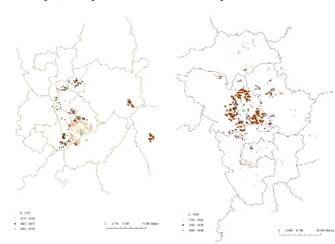
Figures 4a to 4i show maps for each of our nine cities. We use information on a household's

distance to the CBD as well as its income. In order to preserve anonymity, we proceed by

calculating the median income of households living at different percentile distances from

the CBD and assign this income to each household living at this distance27. Some interesting

patterns emerge reflecting the heterogeneity of British cities. In Birmingham, Leeds and

Nottingham there is a clear monocentric pattern, where the poorest households live close

to the CBD with wealthier households located further away; this is also true for Liverpool,

with the caveat that the city is bordered on the west by the River Mersey. In Glasgow this

26

Health status is a five point self-reported scale; we define poor health here as those heads who report being in 'poor' or 'fair' health, as opposed to good, very good or excellent.

27 _{Specifically in these maps each point represents a household, but the marker represents the median income}

12

pattern is almost reversed with an inverse relationship between income and distance from

the CBD. Bristol and Manchester show clear signs of the gentrification of city centres

possibly due to new apartment developments. Here we see largely a positive relationship

between income and distance but with the exception of clusters of high income households

near the city centre. Newcastle and Sheffield show more complex patterns which emerge

from both geography and the economic development of these cities. In Newcastle the

poorest households are in the city centre but these are immediately surrounded by the

richest households, with other low to medium income households further out. Newcastle is

unique in the UK as the site of the first (and arguably only) large-scale example of planning

policies in the late twentieth century with the explicit aim of ‘rebalancing’ the population of

disadvantaged neighbourhoods through ‘positive gentrification’ (Cameron, 2003). Sheffield

has a monocentric pattern, but some of the poorest households are also located in the

outlying ex-mining towns which surround the city.

5. Analysis and results

5.1. Household income and distance from CBD

To analyze the relationship between household income and distance from the CBD we

estimate the following model:

𝑙𝑜𝑔𝐷_𝑖𝑡 = 𝛼 + 𝛽𝑙𝑜𝑔𝑌_𝑖𝑡+ 𝛾′𝑋_𝑖𝑡+ 𝜀_𝑖𝑡 (1)

where i is household, t is wave, D is distance (km) from the CBD, Y is the household’s real

equivalised net income and X is a set of control variables that are described below. Our

focus is the sign of , where a positive value indicates that distance from the CBD increases

with income. This model is estimated using the Stata panel estimator OLS-spatial-HAC

(Hsiang, 2010), which uses the GMM approach outlined by Conley (1999) to take account of

spatial correlation in the error term () for all observations i within a given period. This

13

contain the same households for up to four waves28. A uniform kernel is used to weight

spatial correlations, which falls from 1 to 0 at a cut-off of 50km29.

These results are reported in Table 3 where the main finding is that a household’s income is

positively correlated with distance from the CBD. The associated coefficient is always

significant at conventional levels of significance, regardless of which control variables are

included. Without controlling for any other variable (column 1), the coefficient on log

income is 0.259, suggesting that a 10% increase in income results in a household being

located on average 2.6% further from the city centre. The second column includes city and

wave dummies which make little difference to the coefficient on income. In column (3) we

introduce a set of basic control variables for the age (and age squared), sex, education,

employment and health status of the head of household, as well as whether the household

has children. There is non-linear relationship between age and distance; older people live

further from the CBD, but the rate of increase in distance decreases with age. Households

with children and those with poor health live further from the CBD. There is no significant

relationship between distance from the CBD and the sex of the head of household. The

negative effect of higher education may seem counterintuitive but this may reflect the fact

that household’s income and education are highly correlated (r=0.25, p <0.001). Also it

could be a result of preference for city centre amenities among the highly educated30. Those

households where the head is not employed live closer to the CBD. One explanation,

predicted by job search models (van Ommeren et al, 1999), is that jobs are more readily

found close to the city centre. However, an alternative is that, regardless of job search,

amenities used by those who are not working are more accessible in the city centre. In

column (4) we introduce two additional controls; home ownership and whether the

household is in poverty. Home owners live further from CBD (which is consistent with the

monocentric model which predicts that housing prices decline with distance from the city

28

Note that as many of our households do not move during the time we observe them, it is not appropriate to use a fixed effects estimator. Note also that if we collapse data for those households who do not move to one observation per household using average values across the waves for which they are present in our data, the results are very similar to those presented in Table 3; both significance and size change very little.

29

This means that observations further than 50 km apart are not correlated. Our results are robust to other cut-off distances.

30

14

centre) but there is no significant relationship between distance and being in poverty. The

inclusion of these two variables renders the 'not employed' status of the household head

insignificant, probably due to collinearity, but makes little difference to the other estimates,

and the coefficient on income is reduced slightly.

In column (5) we include two variables relating to the availability of transport; whether or

not the household has access to the car, and a proxy for public transport quality in the

neighbourhood. This latter variable is derived from data from the Department for Transport

that measures how long it takes to travel to various amenities by car and by public

transport31. The data are available at the level of 'lower layer super output area' (LSOA);

these are small neighbourhood areas. There are 32,482 LSOA in England with between 400

and 1200 households in each32. The data give travel times from the centre of each LSOA to

the nearest amenity of each type, so these data give a good indication of travel times for

each of our households. We calculate the ratio of car to public transport travel time, so that

higher values suggest greater availability of public transport. We use travel to the nearest

primary school as our main measure for public transport availability, since we expect

primary schools to be relatively evenly distributed throughout our urban areas, but in our

robustness checks in section 5.3 we also consider travel times to a number of other

amenities33.

Glaeser et al. (2008) argue that one of the reasons why the poor live near the CBD in US

cities is that public transportation to work is more available there and this is important given

the fact that many of the poor do not own their own car; this is also a reasonable

assumption to make about British cities. In our sample of those in poverty only 57% of

households have a car, whereas for those households not in poverty the proportion is 86%.

Our results support Glaeser et al's (2008) argument; those with access to a car live further

away from the CBD and the availability of public transport in the neighbourhood is

associated with living closer to the CBD. The inclusion of these two measures results in a

change in sign for the variable which measures whether or not the head of household is

employed. If we do not take transport availability into account, households where the head

31

www.gov.uk/government/statistics/accessibility-statistics-2013

32 _{The Department for Transport accessibility data that we use for our public transport availability measures is}

only available for England so households in Glasgow are excluded for this part of the analysis.

33

15

is not employed live nearer to the CBD, but after taking into account transport, they live

further away. One explanation for this is that good public transport can reduce the time cost

of travel, reducing the importance of proximity to jobs for the unemployed. Importantly, the

size and significance of the coefficient associated with household income remains very

similar when the public transport variable is included. This result differs from Glaeser et al

(2008) who find that the public transportation explains most of the location of the poor in

U.S cities.

The key finding from Table 3 is that whichever control variables we include in our model the

relationship between distance from the CBD and income remains positive and significant;

although its magnitude is reduced as more control variables are added. In column (5) the

coefficient on log income is 0.123, suggesting that a 10% increase in income results in a

household being located on average 1.2% further from the city centre. At a mean distance

of approximately 8km from the CBD, a 10% increase in income is associated with

households living 0.1 km further away.

5.2. Income Elasticity of Demand for Housing

As discussed above, Becker (1965) shows that the rich choose to live further away from the

CBD if the income elasticity of demand for land is greater than one. To test this hypothesis,

we follow Glaeser et al (2008) and estimate

𝑙𝑜𝑔𝐿_𝑖𝑡 = 𝛼 + 𝜃𝑙𝑜𝑔𝑌_𝑖𝑡 + 𝛿′𝑍_𝑖𝑡+ 𝜈_𝑖𝑡 (2)

As in equation (1) i,t index households and waves, respectively, and Y is the household’s real

equivalised net income. The dependent variable lot size (L) is proxied by the number of

rooms in the accommodation, which is constructed from two questions that ask separately

for the number of bedrooms and the number of 'other' rooms. The conditioning variables

(Z) are the age and sex of the household head, whether or not there are children aged

under 16 living in the household, and whether the resident is an owner occupier; wave and

city dummies are also included34. The focus here is whether is greater than one. Again we

34 _{Note that, in contrast to Glaeser et al's (2008) work for the US, race is not included in our regressions; we}

16

allow for both spatial correlation and autocorrelation in the error term ( by estimating

equation (2) using the spatial panel estimator of Hsiang (2010).

As Glaeser et al (2008) point out, one criticism of using current income in this model is that

this is an error ridden measure of permanent income, and thus the estimate of  is biased

downwards. To overcome this, like Glaeser et al (2008), we instrument for income using

education. The rational for this is that education is correlated with permanent income but

should have no direct effect on housing consumption. Our measure of education is the

highest level of educational attainment gained by the head of household, and this is

represented by a set of dichotomous variables representing O-levels/ GCSEs, A levels, and

degree or higher, with no formal qualifications as the base category35.

The results, which are not reported here for conciseness, show that, whether or not we

instrument for income, house size varies positively with age and is larger when there are

children in the household and for home owners; house size does not vary with the sex of the

household head. Our results for the income elasticity of demand for space are very similar

to those of Glaeser et al (2008) for the US. When we do not instrument for income the

elasticity estimate is very low, at 0.104 (in Glaeser et al the coefficient is 0.08); reducing the

downward bias by instrumenting income with education increases the estimate 0.214 (0.26

in Glaeser et al). Therefore, we conclude that this estimate is too low to explain the

income-distance gradient, as Becker's (1965) model would suggest.

5.3 Robustness checks

To check the robustness of our results we explore six different specifications. Firstly, we

define the CBD using the location of the largest main M&S store rather than the main rail

station. Secondly, we exclude full-time students from our analysis in order to explore

whether our results are affected by the growth in student numbers in cities resulting from

the expansion of higher education. Thirdly, we include only those households where the

head is in employment. Fourthly, we restrict our sample to those households who do not

adjust the dependent variable for household size, calculating rooms per head, the elasticity estimates are very similar to those reported in the text.

35 _{These UK qualification levels largely coincide with finishing education at age 16 (O-levels/ GCSEs), 18 (A}

17

move house during the period of our analysis and are present in all four waves of our data;

here we partly pre-empt the analysis undertaken below on whether or not cities make

people poor. Fifthly, we consider four different definitions of poverty or low income, as an

alternative to the household having less than 60% of median income; these are: being

behind with rent or mortgage; being behind with council tax36; having problems covering all

bills; and the head of household reporting that they are finding it 'difficult to get by'

financially. Finally we consider six alternative public transport access measures; whereas in

Table 3 this variable is the ratio of car to public transport times to primary schools, the

alternative variables measure access (in the same way) to secondary schools, further

education colleges, primary care health services, hospitals, employment centres (with at

least 100 jobs) and town centres.

These results are reported in Table 4 where, for convenience, the first column repeats the

final column (5) from our main specification in Table 3. Defining the CBD as coinciding with

the main M&S store (2) makes virtually no difference the results. Excluding full-time

students (3) results in only a 3% reduction in our sample. The positive income-distance

gradient remains and is slightly steeper than for the full sample. The rest of the coefficients

are similar, with the exception of the one associated with number of children which

becomes insignificant. Employed households (4) make up 68% of our sample. The results for

this sub-sample are very similar to those for the whole sample; the main difference is that

access to car has a larger effect for these households. The sample of non-movers (5) make

up only 41% of the full sample but they have a very similar income-distance gradient to the

full sample. The effects of the control variables are also very similar; the only difference is

that where these households are headed by men they tend to be further from the city

centre. For the four alternative definitions of poverty37; those households where the head

reports they are finding it 'difficult to get by' and those reporting being 'behind with their

council tax' live closer to the CBD. The variables measuring whether or not household is

behind with rent or bills are not statistically significant; one possible explanation for this lack

of significance is that these are not standard definitions of poverty. Similarly using access to

different amenities as alternative measures of public transport makes little difference to the

36 _{The Council Tax in the UK is a system of local property taxation used to partly fund services provided by local}

government.

37

18

results reported in Tables 3 and 4. As a further check on the robustness of our results we

estimate the land elasticity model of equation (2) for the sub-samples of non-movers and

excluding time students; the results are very similar to those reported for the

full-sample above.

In summary our results are robust to variation in the estimation sample, definition of city

centre and to alternative definitions of a number of our explanatory variables. The finding of

a significant positive relationship between distance from the CBD and household income

remains.

5.4 Do cities make people poor?

Our results have so far revealed that poorer households live closer to the city centre. With

our longitudinal data we are also able to address the question of whether British cities tend

to make households poorer or whether they simply attract people who are poor. Here we

follow households who have not changed residence during the analysis period 2009-2013

and analyse how their income has changed over this time period. The concept of spatial

equilibrium implies that, in a frictionless world, households are equally happy in all locations

and hence have no incentives to move. However, another possibility in the real world is that

households do not move because they are constrained and immobile, and thus not able to

satisfy their preferences on location. We can get some idea of which hypothesis is more

likely by exploring their views on their current housing situation. The Understanding Society

survey contains two informative questions in this regard; whether or not the respondent

would prefer to move house, and whether or not they expect to move in the next year. For

our full sample of n= 12,096, 41% would prefer to move and 14% expect to do so. For our

non-mover sample of n = 4,793 a similar proportion (39%) would prefer to move but only

7% expect to do so. This gives some support to the second hypothesis that the non-movers

are more constrained and this explains their geographic immobility. A look at some key

descriptive statistics can partly explain why this might be the case. The two samples have

almost identical proportions of households in poverty, with a car and with children.

However, non-mover households are less likely to have a head who is not in employment

19

households may be constrained by both labour market and housing market circumstances

(Manning, 2003).

Table 5 follows household's income for the non-movers at different distances from the CBD

over the four waves of our sample. This table reveals that on average urban dwellers who

did not move saw virtually no change in their real net income over the period, average

monthly income was £1605 in wave 1 and £1621 in wave 4. However, these figures mask

some variation for households according to distance from the CBD. For those households

who live close to the CBD (between the 1st - 5th and 5th - 25th percentile distance), real

incomes increased. For households further from the CBD real incomes have fallen, with the

exception of those in the furthest percentile distance who saw a small increase. Given that

we have already shown that younger households live closer to the city centre it is tempting

to argue that the growth in income is therefore a result of life stage, with younger people

experiencing faster income growth. However, this is a sample of people who did not move

during the four waves we observe them, and this confounds the age-distance relationship

because younger people are more mobile. The average age of people in each of the first

three distance bands in Table 5 is 45 years, increasing to 46 for the next two bands and 48

for those who live furthest from the CBD. Hence age is not a complete explanation for this

phenomenon. These results provide prima facie evidence that rather than cities making

people poor, they tend to attract poorer people who then experience faster income growth

than those who live further away. However, it is worthy of note that real incomes in the

nearest percentile distance (£1404) are still only 85% of those in the furthest percentile

(£1652) in wave 4.

6. Conclusions

In this paper we present the first study that has explored the relationship between income

and the location of urban households in Britain. Our findings show that the poorest

households tend to live closer to the CBD than the rest of urban dwellers. Moreover, after

controlling for several household characteristics and access to transport (as well as city and

20

household’s income and distance from the CBD. We test whether the income elasticity for

the demand for housing is large enough to conclude that richer households live further

away from the CBD to consume larger dwellings. Our results show that this elasticity is much

lower than one and so preference for space cannot fully explain our findings on the

income-location pattern. These results are very similar to those of Glaeser et al. (2008) for the US;

and they contrast with those of Brueckner et al (1999) who argue that the US pattern, for

those with higher wages to choose to live further from the CBD, is reversed in Europe where

amenities are concentrated in historic city centres. However, unlike Glaeser et al (2008) we

do not find that public transport availability can explain the spatial distribution of income.

Finally, using a subsample of households who did not change residence over the time period

analysed, we find some evidence that households who live closer to the CBD are the ones

who have experienced the largest increases in real income over the period. This suggests

that one can reject the hypothesis that cities tend to make households poor, and may even

conclude that cities are good for the poor. However, importantly for urban planning

debates, those who live near the CBD are still poor relative to those who live further away.

References

Ahlfeldt, G., and N. Wendland (2014), “How Polycentric is a Monocentric City? The Role of Agglomeration Economies,” Journal of Economic Geography 13(1): 53-83.

Ahlfeldt, G., K. Moller, S. Waights, and N. Wendland (2014), “The Economics of Conservation Area Designation,” manuscript.

Alonso, W. (1964), Location and Land Use. Harvard University Press.

Becker, G.S. (1965), “A Theory of the Allocation of Time,” Economic Journal 75: 493-508.

Beckman, M.J. (1974), “Spatial Equilibrium in the Housing Market,” Journal of Urban Economics 1, 99-107.

Bowden, M. (1971), “Downtown through Time: Delimitation, Expansion, and Internal Growth,” Economic Geography47(2): 121–135.

Brown, S. (1987), “The Complex Model Centre of City Retailing: an Historical Application,”.

Transactions of the Institute of British Geographers 12(1): 4–18.

21

Brueckner, J., and S. Rosenthal (2009), “Gentrification and Neighborhood Housing Cycles: Will America’s Future Downtowns Be Rich?” Review of Economics and Statistics 91(4): 725-743.

Brueckner, J., J-F. Thisse, and Y. Zenou (1999), “Why is Central Paris Rich and Downtown Detroit Poor? An Amenity-Based Theory,” European Economic Review 43: 91-107.

Cameron, S. (2003). Gentrification, housing redifferentiation and urban regeneration: “Going for Growth” in Newcastle upon Tyne. Urban Studies, 40(12), 2367–2382.

Carr, J., Councell, R., Higgs, M., Singh N. (2014) Households below average income: an analysis of the income distribution1994/95 – 2012/13. Department for Work and Pensions. https://www.gov.uk/government/statistics/households-below-average-income-hbai-199495-to-201213

Conley, T.G. (1999) GMM estimation with cross sectional dependence. Journal of Econometrics, 92(1): 1-45

Cribb, J.. Hood, A., Joyce, R., Philips, D. (2013) Living Standards, Poverty and Inequality in the UK: 2013. Report R81. London: Institute for Fiscal Studies.

DETR [Department of the Environment, Transport and the Regions] (2000). Our towns and cities: The future . London: HMSO

Frank, R., (1985), Choosing the Right Pond. Oxford University Press. New York.

Fujita, M. (1989), Urban Economic Theory. Cambridge University Press, Cambridge, UK.

Galster, G., (2005),“Consequences from the Redistribution of Urban Poverty in the 1990s: a Cautionary Tale,” Economic Development Quarterly 19(2): 119-25.

Galster, G., Marcotte, D.E., Mandell, M., Wolman, H. and August, N. (2007), “The Influence of Neighbourhood Poverty during Childhood on Fertility, Education and Earnings Outcomes,” Housing Studies 22(5): 723–751.

Giuliano, G., and K.A. Small (1991), “Subcenters in the Los Angeles Region.” Regional Science and Urban Economics 21: 163-182.

Glaeser, E.L, M.E. Kahn, and J. Rappaport (2008), “Why Do the Poor Live in Cities? The Role of Public Transportation.” Journal of Urban Economics 63: 1-24.

Gutiérrez-i-Puigarnau, E., Mulalic, I., & van Ommeren, J. (2014). Do rich households live farther away from their workplaces ? Journal of Economic Geography, 1–25

Henderson, J.V. (1977). Economic Theory and the Cities. Academic Press, New York, USA.

22

Hsiang SM (2010) Temperatures ad cyclones strongly associated with economic production in the Caribbean and Central America. Proceedings of the National Academy of Science of the United States of America. 107(35):15367-72.

Hunter P. (2014) Poverty in suburbia: A Smith Institute study into the growth of poverty in the suburbs of England and Wales. London: Smith Institute.

Kantor, Y., P. Rietveld, and J. van Ommeren (2014), “Towards a General Theory of Mixed Zones: The Role of Congestion.” Tinbergen Institute Discussion Paper TI 2013-084/VIII

LeRoy, S.F. and J. Sonstelie (1983), “Paradise Lost and Regained: Transportation Innovation, Income, and Residential Location.” Journal of Urban Economics 13: 67-89.

Manning, A. (2003). The real thin theory: monopsony in modern labour markets. Labour Economics 10 (2), 105-131

McKinnish, T., R. Walsh, and T.K. White (2010), “Who Gentrifies Low-Income Neighborhoods?” Journal of Urban Economics 67(2): 180-193.

Mills, E.S. (1967), “An Aggregative Model of Resource Allocation in a Metropolitan Area.”

American Economic Review 57: 197-210.

Muth, R.F. (1969), Cities and Housing. University of Chicago Press.

Nathan, M., Urwin, C., Champion, A., & Morris, J. (2005). City People: City centre living in the UK. London: Institute for Public Policy Research

Ng, C.F. (2008), “Commuting Distances in a Housing Location Model with Amenities.”

Journal of Urban Economics 63, 116-129.

Patacchini, E., and Y. Zenou (2006), “Search Activities, Cost of Living, and Local Labor Markets.” Regional Science and Urban Economics 36: 227-248.

Persky, J. (1990), “Suburban Income Inequality,” Regional Science and Urban Economics 20: 125-137.

Rae, A. (2009), “Isolated Entities or Integrated Neighbourhoods: an Alternative Approach to the Measurement of Deprivation,” Urban Studies 46(9): 1859-78.

Rae, A. (2012), “Spatially Concentrated Deprivation in England: An Empirical Assessment,”

Regional Studies 46(9): 1183–1199.

Rae, A. (2013), “English Urban Policy and the Return to the City: a Decade of Growth, 2001-2011,” Cities 32: 94-101.

Rappaport, J. (2014), “Monocentric City Redux,” Federal Reserve Bank of Kansas City Research Working Paper, RWP, 14-09.

23

Schiller, R. (2001), The Dynamics of Property Location. London: Verso.

Tallon, A., and R. Bromley (2004), “Exploring the Attractions of City Centre Living: Evidence and Policy Implications in British Cities,” Geoforum 35(6): 771–787.

Taylor MF (ed). with Brice J, Buck N, Prentice-Lane E. (2010) British Household Panel Survey User Manual Volume A: Introduction, Technical Report and Appendices. Colchestre: University of Essex.

Townsend, I., and S. Kennedy (2004), Poverty: Measures and Targets. Research Report 04/23. House of Commons Library.

University of Essex (2015). Institute for Social and Economic Research and NatCen Social Research,

Understanding Society: Waves 1-4, 2009-2013: Secure Access [computer file]. 4th Edition. Colchester, Essex: UK Data Archive [distributor. SN: 6676, http://dx.doi.org/10.5255/UKDA-SN-6676-4.

Van Ommeren, J., Rietveld, P., & Nijkamp, P. (1999). Job Moving, Residential Moving, and Commuting : Journal of Urban Economics, 230–253.

24

Table 1: Number of households and mean income by city and wave

City 2011 Wave 1 Wave 2 Wave 3 Wave 4

population Households Income1 Households Income1 Households Income1 Households Income1

Birmingham 1073045 706 1399 564 1497 507 1462 481 1509

Bristol 428234 247 1647 234 1557 207 1697 210 1628

Glasgow 629501 358 1699 383 1824 334 1668 303 1704

Leeds 751485 285 1353 235 1439 199 1518 175 1539

Liverpool 466415 261 1629 237 1711 213 1690 194 1685

Manchester 503127 411 1604 366 1602 319 1612 290 1668

Newcastle 280177 372 1485 345 1568 310 1563 300 1549

Nottingham 305680 403 1547 398 1443 374 1472 347 1490

Sheffield 552698 408 1478 412 1503 381 1518 328 1515

Total 4990362 3451 1522 3174 1566 2844 1569 2628 1576

1

25

Table 2: Descriptive statistics at different distances from the CBD, for household (HH) and head of household (HoH).

Percentile distance from CBD Number of households Distance from CBD (km) Mean monthly HH income (£)1 HH in poverty2 (%) HoH not employed (%) HoH has Higher Education (%) Children in HH (%) Average age of HoH (years) HoH is male (%) Hoh in poor health (%) Number of rooms in home HH owns home (%) HH has a car (%) < 5 601 < 1.82 1399 47.7 43.7 38.1 25.2 32 59.7 19.1 3.5 23.6 48.1 5-25 2415 1.82 -

3.96

1377 49.6 37.3 39.1 41.7 40 54.4 23.0 4.4 50.6 66.1

25-50 3023 3.96 - 6.63

1567 39.6 31.5 37.8 41.7 44 56.7 22.7 4.6 60.5 75.0

50-75 3027 6.63 - 10.72

1657 33.3 30.2 32.8 39.9 45 57.6 23.4 4.7 66.0 78.6

75-95 2422 10.72 - 2.70

1620 31.9 28.1 32.7 37.6 45 61.5 19.7 4.7 70.3 82.9

>95 608 > 22.70 1613 30.5 27.3 26.9 34.3 46 67.9 19.9 4.8 69.2 86.3

26

Table 3: Household income and distance from the CBD.

Dep. var. Log distance (1) (2) (3) (4) (5)

Household income 0.259*** 0.258*** 0.123*** 0.105*** 0.123*** (0.003) (0.004) (0.016) (0.012) (0.014)

Age 0.034** 0.039*** 0.043***

(0.005) (0.004) (0.004)

Age squared -0.000*** -0.000*** -0.000***

(5.2-05) (3.9e-05) (4.0e-05)

Sex 0.023 0.006 0.001

(0.022) (0.020) (0.021)

Higher education -0.137*** -0.167*** -0.183***

(0.017) (0.018) (0.019)

Children 0.091*** 0.077*** 0.044**

(0.018) (0.017) (0.018)

Not employed -0.081*** -0.008 0.046**

(0.021) (0.021) (0.019)

Health 0.023*** 0.016** 0.016**

(0.006) (0.007) (0.008)

Home owner 0.198*** 0.150***

(0.026) (0.029)

In poverty -0.041 -0.015

(0.026) (0.021)

Access to car 0.187***

(0.015)

Public transport access -0.434***

(0.066)

City and wave dummies no yes yes yes

Observations 12,096 12,096 12,082 12,082 10,691

R-squared 0.860 0.864 0.873 0.874 0.876

27

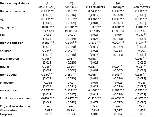
Table 4: Household income and distance from the CBD: Robustness checks.

Dep. var. Log distance (1) (2) (3) (4) (5)

Table 3. Col (5) M&S CBD Ex. FT students Employed Non-movers Household income 0.123*** 0.118*** 0.143*** 0.138*** 0.110***

(0.014) (0.016) (0.015) (0.009) (0.015)

Age 0.043*** 0.045*** 0.036*** 0.038*** 0.049***

(0.004) (0.004) (0.004) (0.001) (0.006)

Age squared -0.000*** -0.000*** -0.000*** -0.000*** -0.000*** (4.0e-05) (4.4e-05) (4.1e-05) (1.7e-05) (6.3e-05)

Sex 0.001 -0.010 0.014 -0.007 0.045**

(0.021) (0.019) (0.022) (0.018) (0.018)

Higher education -0.183*** -0.194*** -0.178*** -0.207*** -0.177***

(0.019) (0.020) (0.019) (0.022) (0.022)

Children 0.044** 0.049*** 0.021 0.018 -0.007

(0.018) (0.018) (0.017) (0.013) (0.010)

Not employed 0.046** 0.037* 0.098*** 0.068***

(0.019) (0.020) (0.023) (0.010)

Health 0.016** 0.014* 0.027*** 0.027*** 0.024**

(0.008) (0.008) (0.006) (0.007) (0.011)

Home owner 0.150*** 0.157*** 0.145*** 0.141*** 0.136***

(0.029) (0.030) (0.031) (0.030) (0.038)

In poverty -0.015 -0.024 0.004 -0.021 -0.018

(0.021) (0.021) (0.022) (0.029) (0.032)

Access to car 0.187*** 0.192*** 0.186*** 0.285*** 0.177***

(0.015) (0.017) (0.017) (0.036) (0.025)

Public transport access -0.434*** -0.447*** -0.436*** -0.409*** -0.378***

(0.066) (0.068) (0.072) (0.077) (0.060)

City and wave dummies yes yes Yes Yes Yes

Observations 10,691 10,691 10,344 7,267 4,401

R-squared 0.876 0.873 0.880 0.886 0.889

28

Table 5: Income evolution over time across distances from CBD. All non-mover households

Percentile distance from CBD

Income Income Change (%)

wave 1 wave 2 wave 3 wave4 w1-w2 w2-w3 w3-w4 w1-w4

<5 1347 1361 1513 1404 1.04 11.17 -7.20 4.23

5-25 1472 1518 1523 1619 3.13 0.33 6.30 9.99

25-50 1644 1614 1639 1633 -1.82 1.55 -0.37 -0.67

50-75 1684 1610 1622 1637 -4.39 0.75 0.92 -2.79

75-95 1653 1660 1659 1634 0.42 -0.06 -1.51 -1.15

>95 1611 1512 1633 1652 -6.15 8.00 1.16 2.55

Total 1605 1586 1609 1621 -1.18 1.45 0.75 1.00

29

Figure 1: possible locations of the poor and the rich in the monocentric model

Distance from the CBD Household

income

Rich

Poor

Distance from the CBD Household

income

Poor

Rich

Source: Adapted from (Brueckner, 2011)

Figure 2: The distribution of household income

30

Figure 3: Histogram of households’ distances (km) to the CBD

31

32

33