Cyclic multicategories, multivariable adjunctions and mates

This is a repository copy of Cyclic multicategories, multivariable adjunctions and mates.

White Rose Research Online URL for this paper:

http://eprints.whiterose.ac.uk/98611/

Version: Accepted Version

Article:

Cheng, E., Gurski, N. and Riehl, E. (2014) Cyclic multicategories, multivariable adjunctions

and mates. Journal of K-Theory, 13 (02). pp. 337-396. ISSN 1865-2433

https://doi.org/10.1017/is013012007jkt250

[email protected]

Reuse

Unless indicated otherwise, fulltext items are protected by copyright with all rights reserved. The copyright exception in section 29 of the Copyright, Designs and Patents Act 1988 allows the making of a single copy solely for the purpose of non-commercial research or private study within the limits of fair dealing. The publisher or other rights-holder may allow further reproduction and re-use of this version - refer to the White Rose Research Online record for this item. Where records identify the publisher as the copyright holder, users can verify any specific terms of use on the publisher’s website.

Takedown

If you consider content in White Rose Research Online to be in breach of UK law, please notify us by

Cyclic multicategories, multivariable adjunctions

and mates

Eugenia Cheng, Nick Gurski and Emily Riehl

Department of Mathematics, University of Sheffield

E-mail: [email protected], [email protected]

and

Department of Mathematics, Harvard University

E-mail: [email protected]

April 15, 2016

Abstract

A multivariable adjunction is the generalisation of the notion of a 2-variable adjunction, the classical example being the hom/tensor/cotensor trio of functors, ton+ 1 functors ofnvariables. In the presence of

multi-variable adjunctions, natural transformations between certain composites built from multivariable functors have “dual” forms. We refer to corre-sponding natural transformations as multivariable or parametrised mates, generalising the mates correspondence for ordinary adjunctions, which en-ables one to pass between natural transformations involving left adjoints to those involving right adjoints. A central problem is how to express the naturality (or functoriality) of the parametrised mates, giving a precise characterization of the dualities so-encoded.

We present the notion of “cyclic double multicategory” as a structure in which to organise multivariable adjunctions and mates. While the stan-dard mates correspondence is described using an isomorphism of double categories, the multivariable version requires the framework of “double multicategories”. Moreover, we show that the analogous isomorphisms of double multicategories give a cyclic action on the multimaps, yielding the notion of “cyclic double multicategory”. The work is motivated by and applied to Riehl’s approach to algebraic monoidal model categories.

Contents

2 Multivariable adjunctions 13

2.1 Definition of multivariable adjunctions . . . 14

2.2 A motivating example . . . 20

2.3 Composition . . . 22

2.4 Multivariable mates . . . 27

3 Cyclic double multicategories 35 3.1 Plain multicategories . . . 35

3.2 Cyclic multicategories . . . 37

3.3 Cyclic double multicategories . . . 42

3.4 Multivariable adjunctions . . . 44

4 Application to algebraic monoidal model categories 48

Introduction

Frequently in homotopical algebra and algebraic K-theory, one is dealing with model categories with extra structure. In particular, the model structure is often required to be compatible with a closed monoidal structure on the underlying category or an enrichment over another model category. For instance, enriched model categories play an essential role in equivariant homotopy theory [8, 9, 10]. The formal definitions, introduced in [12], generalize Quillen’s notion of a simplicial model category and can be expressed in three equivalent (“dual”) forms. Although these formulations are well-known, the precise nature of these dualities is not obvious because they involve a two-variable adjunction defined on arrow categories constructed from a two-variable adjunction on the underlying categories and an associated bijective correspondence between certain natural transformations that has never been precisely described.

Indeed, a fully satisfactory account of the dualities for natural transforma-tions involving a “tensor/cotensor/hom” trio of functors demands a general-ization from two-variable adjunctions to multivariable adjunctions: the ten-sor/cotensor/hom combine with the closed monoidal structure on the enrich-ing category to define functors ofn-variables with compatibly defined adjoints. Again, in the presence of multivariable adjunctions, natural transformations between certain composites built from multivariable functors (e.g. encoding co-herence conditions) have “dual” forms. This sort of structure occurs in work

of the third author in the context of monoidal and enriched algebraic model

category structures [23, 24]. In an algebraic model category structure, the weak factorisation systems involved have certain extra linked algebraic/coalgebraic structure; all cofibrantly generated model categories can be made algebraic in this sense. That research was one direct motivation for the work and results in this paper, which are essential to define the central notion studied in [24].

involving these sorts of natural transformations will have “dual” forms. Our re-sult makes this precise. Before giving a more detailed description of the problem and an outline of our solution, let us introduce a key idea via an analogy.

The pervasive success of homology theories stems from an abstract frame-work that simultaneously enables computation and generalisation. For example, homology originated from the study of invariants of topological spaces and was extended to associative algebras, Lie algebras, and the extraordinary homology theories appearing in stable homotopy theory, such as K-theory and cobordism. In these settings, we often start with some basic objects, and then consider additional algebraic structure. Operads are a powerful tool for encoding such structure. This is witnessed by the great progress made in the theory of iterated loop spaces [22] and topological field theories [5], for example.

While operads can be used to generalise notions of algebraic structure, there is still a further useful generalisation: operads themselves come in different flavours, allowing us to embrace yet further notions of algebra. One major example of this is Getzler and Kapranov’s notion of cyclic operad. This was introduced in order to generalise cyclic homology to these further types of alge-bras.

The “cycles” at play here are cycles of inputs and outputs. That is, where operads encode algebraic operations, cycles enable us to exchange inputs and outputs of these operations. One natural way in which such structure arises is in the presence of duality. For example, for finite-dimensional vector spaces, a linear map

F: V W

corresponds precisely to a map between the duals in the opposite direction, that is

F∗ :W∗

V∗

.

Of course, vector spaces form not merely a category, but a monoidal category, and the tensor product interacts with the duality as follows. A linear map

V1⊗V2⊗ · · · ⊗Vn V0

corresponds precisely to one as shown below

V2⊗ · · · ⊗Vn⊗V

∗

0 V

∗

1

where the “output” vector space has been exchanged with one of the “inputs”, and those two spaces are dualised. We can repeat this process and “cycle” the inputs and outputs round as many times as we like. In this sense the basic version above is the 1-ary version of this cyclic process, which we can do for any

n≥1.

A categorical version of duality is given by adjunctions. An adjunction

A ⊥ B

F

is given by the same data as an adjunction

Bop ⊥ _Aop_.

Gop

Fop

As for vector spaces, categories form a monoidal category via the cartesian product, and we seek the correctn-ary version of adjunctions.

A ubiquitous example of a 2-variable adjunction is the tensor/hom/cotensor trio of functors mentioned earlier. The tensor/hom adjunction

⊗b⊣[b , ]

is particularly familiar, and in many enriched cases there is further adjoint, the cotensor

a⊗ ⊣a⋔

These three functors⊗,[ , ],⋔_{are related by adjunctions in a way that looks}

somewhat convoluted at first sight. It has the following features:

it involves 3 functors of 2 variables,

each pair of functors is related by a 1-variable adjunction if we fix a vari-able, and

some care is required over dualities of source and target categories.

In fact, when treated cyclically, the structure becomes transparent; we discuss it in detail in Section 2.2. While the functors in this example have only two variables, composing them results in new functors of higher arity. In fact, any tensored and cotensored category enriched in a closed symmetric monoidal cat-egory admits ann-variable adjunction for each natural numbern, encoding the interaction between these structures.

Two-variable adjunctions appear in the statement of the pushout-product axiom, which is the crucial component of the definition of a simplicial, or more generally enriched, model category. It is well known that there are three equiv-alent formulations of this axiom that are somehow dual. The key to this duality is that in the presence of pushouts and pullbacks, the arrow categories admit adjunctions similar to the tensor/hom/cotensor trio. The three cyclic adjoints yield the three forms of the pushout-product axiom. Multivariable adjunctions of this sort are also used in higher category theory, for instance, to define the lifting properties characterising an n-fold quasi-category, a presheaf model for an (∞, n)-category [11].

In fact we desire a richer structure than just multicategories because the “duality” involved in adjunctions extends to 2-cells as well—natural transfor-mations involving left adjoints become natural transfortransfor-mations involving right adjoints via the “mates correspondence”. This 2-dimensional duality is at the heart of the three equivalent formulations of an algebraic formulation of the simplicial model category axioms mentioned above.

The mates correspondence is elegantly described using the framework of double categories. Recall that a double category is a form of 2-dimensional cat-egory with two types of morphism—horizontal and vertical—and 2-cells that fit inside squares. The double category used to describe the mates correspondence is given as follows:

0-cells are categories,

horizontal 1-cells are functors,

vertical 1-cells are adjunctions (pointing in a fixed chosen direction e.g. the direction of the left adjoint), and

2-cells are certain natural transformations.

Even after we have fixed the direction of the 1-cells, there is a choice for the 2-cells—we could still take the natural transformations to live in the squares involving either the left or right adjoints. This producesa priori two different double categories for each choice of 1-cell direction, but the mates correspon-dence says precisely that there is an isomorphism of double categories between them.

For multivariable adjunctions we thus need to combine the notions of mul-ticategory, double category, and cyclic action. Our vertical 1-cells will now be

n-variable adjunctions, so they are the maps of a multicategory with a cyclic action. For example a 2-variable adjunction involves functors

A×B−→F Cop B×C−→G Aop C×A−→H Bop_.

Note the duality that arises as a category “cycles” between the source and target. The essential fact is that each time a category moves between the source and target, it is dualised; this is exactly what happens for vector spaces, and in the tensor/hom/cotensor situation. This is the notion of a “cyclic multicategory”— a multicategory equipped with additional structure in the form of

an involution (such as ( )op_{), and}

a cyclic action on homsets, invoking the involution appropriately.

This formulation allows for cyclic structures that do not arise from duals in the

sense of dual vector spaces, such n-variable adjunction. (Note that opposite

We must also implement the cyclic structure on 2-cells, that is, then-variable version of the mates correspondence. We are interested in a correspondence of natural transformations such as below (for the 2-variable example):

A×B A′

×B′

Cop _C′op

F F′

B×C B′

×C′

Aop _A′op

G G′

C×A C′

×A′

Bop _B′op

H H′

and this indicates the required form of 2-cells and their cyclic structure, in our “cyclic double multicategory”. Recall that a double category can be defined succinctly as a category object inCat; similarly a cyclic double multicategory is a category object in the category of cyclic multicategories.

The motivation for this work is the third author’s work on algebraic monoidal model categories. In the theory of algebraic model categories [23] the double cat-egory framework for 1-variable adjunctions and mates plays a crucial role. For the monoidal version [24], multivariable adjunctions and mates are needed, not simply to describe the equivalent forms the definition of a monoidal algebraic model category might take but to state the correct definition at all. Exam-ples that could now be made algebraic using the results of the present paper include the model structures arising from 2-category theory [18], in particular the monoidal model structure on 2-categories with the Gray tensor product [16, 17]. Similar ideas applied in the context ofn-fold quasi-categories would give an “algebraic” model for (∞, n)-categories.

This paper is organised as follows. In Section 1 we recall the standard theory of mates. In Section 2 we define multivariable adjunctions and the multivari-able mates correspondence. In Section 3 we give the definition of cyclic double multicategory, building up gradually through multicategories, cyclic multicat-egories and double multicatmulticat-egories. We show that multivariable adjunctions form a cyclic double multicategory. In Section 4 we describe the application to algebraic monoidal model categories.

Our notion of cyclic multicategory is non-symmetric and thus generalises the notion of (non-symmetric) cyclic operad given in [1]; symmetric cyclic operads are defined in [4] and a multicategory version is mentioned in [13]. Our defi-nition could also be given in a symmetric form but we felt that the new ideas introduced here were highlighted most clearly when the obvious symmetries of

the cartesian product on CAT were ignored. Cyclic operads support a wide

variety of applications, as described in the papers [1] and [4], and so we expect the categorical formalism encoded by our “coloured” version presented here will also be useful in other contexts.

Notation

Throughout this paper we will writeA•

forAop. Also, forn-variable adjunctions and cyclic multicategories, we will need to use subscripts cyclically. Thus we will index objects by 0, . . . , nwith lists taken cyclically, modn+ 1. For example we will frequently use the stringai+1, . . . , ai−1 which means

ai+1, ai+2, . . . , an, a0, a1, . . . , ai−1.

Acknowledgements

The third author was supported by both the NSF Graduate Research Fellowship Program and an NSF Mathematical Sciences Postdoctoral Research Fellowship. She also had useful conversations with Anthony Elmendorf, Daniel Sch¨appi, and Dominic Verity. This work was catalysed by a visit partially sponsored by the University of Sheffield Mathematical Sciences Research Centre.

1

Mates

In this section we describe the situation we will be generalising. Suppose we have the following categories, functors and adjunctions

A

B

⊣

F G

A′

B′ ⊣

F′ _G′

with unit and counit (η, ε) and (η′

, ε′

) respectively. Then given functorsS and

T and a natural transformationαas shown

A A′

B B′

S

T

F α F′

itsmate α¯ is the natural transformation

A A′

B B′

S

T

G G′

¯

α

B A A′

B B′

A′ . G 1 S T

F F′ 1

G′ α

ε

η′

Conversely we can start with

A A′

B B′

S

T

G G′

β

and obtain the mate

A A′

B B′

S

T

F F′

¯

β

as the composite

A

A A′

B B′_.

B′

1

F

S

T

G G′

F′

1

β ε

η′

By triangle identities these processes of “conjugation” are inverse to one an-other. Furthermore, the correspondence respects both horizontal and vertical composition in the following sense. Given adjunctions

A1

B1

⊣

F1 G1

A2

B2

⊣

F2 G2

A3

B3

⊣

F3 G3

and natural transformations

A1 A2 A3

B1 B2 B3

S1

T1

S2

T2 F1 α1 F2 α2 F3

we have

where ∗ is to be interpreted with the appropriate whiskering, so in fact the honest equality is

T2α1◦α2S1=α2T1◦S2α1.

For “vertical” composition, given adjunctions

A1

B1

C1

⊣

F1 G1

⊣

H1 K1

A2

B2

C2

⊣

F2 G2

⊣

H2 K2

and natural transformations

A1 A2

B1 B2

C1 C2

S

T

U F1

H1

F2

H2 α1

α2

we have

α2◦α1=α2◦α1

which actually means

α2F1◦H2α1=G2α2◦α1K1.

Both of these facts are easily checked using 2-pasting diagrams and triangle identities.

This situation is conveniently formalised using double categories. In the following definition we have chosen the direction of the vertical 1-cells to corre-spond to the direction of the left adjoints.

Definition 1.1. We define two double categories L_{Adj and} R_{Adj with the}

same 0- and 1-cells, but different 2-cells. In both cases the 0-cells are categories, the horizontal 1-cells are functors, and a vertical 1-cellA Bis an adjunction

A ⊥ B.

F

A 2-cell _A

1 A2

B1 B2

S

T

⊣

F1 G1 F2 ⊣ G2

is given in each case as follows.

InL_{Adjsuch a 2-cell is a natural transformation}

A1 A2

B1 B2.

S

T

F1 F2

α

InR_{Adjsuch a 2-cell is a natural transformation}

A1 A2

B1 B2.

S

T

G1 _α G2

Theorem 1.2. [15, Proposition 2.2]

There is an isomorphism of double categories

L_Adj∼₌R_Adj

which is the identity on 0- and 1-cells (horizontal and vertical); on 2-cells it is given by taking mates.

We now look at this from a slightly different point of view that seems a little contrived here, but leads to a natural framework for then-variable generalisa-tion. The idea is to notice that an adjunction

A ⊥ B

F

G

is equivalently an adjunction

B• _{⊥ A}•_.

G•

F•

Now, we could deal with this by introducing yet another pair of double categories

L_{AdjR and}R_{AdjRas above but whose vertical 1-cells point in the direction of}

theright adjoints; the 2-cell directions must also be changed accordingly. We would then get isomorphisms of double categories

( )•_{:LAdj−→RAdj}

R

( )•_{:RAdj−→LAdj}

However, we can actually express all this structure using one single version of the above four isomorphic double categories, as follows.

Given a 2-cell inL_{Adj, that is, a natural transformation}

A1 A2

B1 B2

S

T

F1 F2

α

its mate

A1 A2

B1 B2

S

T G1 _α¯ G2

is not a priori a 2-cell of L_{Adjas its source and target involve right adjoints} G1 andG2. However, it can be dualised to give

A•

1 A

•

2

B•

1 B

•

2

S•

T• G•

1 G•2

¯

α•

where we must reverse the 2-cell direction as the target category has been du-alised. Thus, turning the diagram round so that the left adjoints point down-wards, we have

A•

1 A•2 B•

1 B2•

S• T•

G•

1 G•2

¯

α•

which is a 2-cell of L_{Adj as G}•

1 and G•2 are left adjoints. Thus the mates

correspondence actually gives us some extra structure on L_{Adj in the form of}

isomorphisms:

L_{Adjv(A, B)}∼₌L_Adjv(B•_{, A}•_{), and}

L_{Adj2(S, T)}∼₌L_Adj2(T•_{, S}•_).

Definition 1.3. Consider functors

A F B•

so A• F•

B B G A•

B• G•

A.

Amutual left adjunctionofF andGis an adjunction

F•

⊣G

or equivalently

G•

⊣F.

Note that this is given by isomorphisms

B(F a, b)∼=A(Gb, a) natural inaandb. If we started with

A• F _{B and}

B• G _A

then the adjunctions

F•

⊣G or G•

⊣F

as above would be given by isomorphisms

B(b, F a)∼=A(a, Gb),

which is called amutual right adjoint.

Note that the unit and counit for a mutual left adjoint as above have com-ponents

ηa:GF a a∈A and εb:F Gb b∈B,

whereas for a mutual right adjoint the components are

ηa:a GF a∈A and εb:b F Gb∈B.

Remark 1.4. The unit and counit given above are for an adjunction

F•

⊣G

whereas for the (equivalent) adjunction

G•

⊣F

the unit and counit are the other way round, that is,

εa:GF a a∈A and ηb:F Gb b∈B.

We can now express the mates correspondence for mutual left adjunctions. Given a mutual left adjunction between

A F B• _and

B G A•

the mates correspondence together with duality as above gives us a correspon-dence between natural transformations

A A′

B• _B•

S

T•

F F′ _and

B B′•

A•

A′•_.

T

S•

G G′

This is obtained from the ordinary mates correspondence by taking some ap-propriate duals. This is then= 1 part of then-variable case, in which we look at natural transformations

A1× · · · ×An A′1× · · · ×A

′

n

A•

0 A′0

•

S1× · · · ×Sn

S• 0

and

A2× · · · ×A0 A′2× · · · ×A′0

A•

1 A′1

•

S2× · · · ×S0

S• 1

and every cyclic variant.

2

Multivariable adjunctions

In this section we define multivariable adjunctions. The basic idea is that for an “n-variable adjunction” we have n+ 1 categories A0,· · ·, An and n+ 1

multifunctors, each of which has one of theA•

i as its target, and the product of

the othern categories as its source. These multifunctors can all be restricted to functors with a single category as their source, by fixing an object in each of the other categories. For every pair i 6= j there is a pair of contravariant functors obtained in this way involvingAiandAj. These should be in a specified

We first give the definition of this structure, and then immediately prove

Theorem 2.2 giving a more “economical” characterisation, in whicha priori we

specify only one multifunctor, and a family of 1-variable adjoints for it. Using standard results about parametrised representability, these 1-variable adjoints then extend uniquely ton-variable multifunctors with the required structure. It is the characterisation in Theorem 2.2 that we will use in the rest of the work.

2.1

Definition of multivariable adjunctions

Definition 2.1. Let n ∈ N_{. An n-variable (mutual) left adjunction is}

given by the following data and axioms.

CategoriesA0, . . . , An.

Functors

A1×A2× · · · ×An−1×An F0

A•

0 A2×A3× · · · ×An×A0

F1

A•

1

.. .

Ai+1× · · · ×Ai−1

Fi

A•

i

.. .

A0× · · · ×An−1

Fn

A•

n.

Here the subscripts are all to be taken mod n+ 1. Where possible, we

will adopt the convention that the subscript on a multifunctor matches the subscript of its target category.

For all 0≤i≤n, and for all ai+1 ∈Ai+1, . . . , ai−2∈Ai−2 a mutual left

adjunction between

Ai A

•

i−1

Ai−1 A•i

Fi−1( , ai+1, ai+2, . . . , ai−2)

Fi(ai+1, ai+2, . . . , ai−2, )

thus isomorphisms

Ai−1 Fi−1(ai, . . . , ai−2), ai−1

_∼

=Ai Fi(ai+1, . . . , ai−1), ai

natural in ai−1 and ai. If we use the shorthand ˆai for the sequence ai+1, . . . , ai−1, this isomorphism takes the appealing form

Ai−1 Fi−1(ˆai−1), ai−1∼=Ai Fi(ˆai), ai

.

The following axioms must be satisfied:

the “cycle” of isomorphisms commutes:

An Fn(ˆan), an

A0 F0(ˆa0), a0

A1 F1(ˆa1), a1

A2 F2(ˆa2), a2

A3 F3(ˆa3), a3 ..

.

. ..

∼

∼

∼

∼ ∼

We say that the functor F0 is equipped with n-variable left adjoints

F1,· · ·, Fn. This terminology makes more sense in the light of the following

theorem.

Theorem 2.2. The following description precisely corresponds to ann-variable left adjunction.

categories A0, . . . , An

a functorA1× · · · ×An F0

A•

0

for all 0, j, k distinct, and for all aj ∈ Aj, a mutual left adjoint for the

functor

F0(a1, . . . , ak−1, , ak+1, . . . , an) :Ak A•0

Remark 2.3. Note we say that F is equipped withn-variable left adjoints if each of its 1-variable restrictions has a leftadjoint. F is equipped with n -variablerightadjoints if each of its 1-variable restrictions has arightadjoint.

To prove this we use the following result of Mac Lane [20, IV.7, Theorem 3].

Theorem 2.4. Given categoriesA, B, C, a functorF:A×B C•

, and for allb∈B a mutual left adjoint G(b, ) :C A•

for the functor

F( , b) :A C•

i.e. isomorphisms

C(F(a, b), c)=∼A(G(b, c), a) (1)

natural ina andc, there is a unique way to extend the functors

G(b, ) :C A•

to a single functor

G: B×C A•

This is a standard result about parametrised representability; we give a 2-categorical expression of Mac Lane’s proof, as this will be useful later.

Proof. We write 1 b B for the functor picking out the objectb ∈ B. The hypothesis of the theorem then says that for each suchbwe have a right adjoint for the composite

A• _A•

×B•

C 1×b• _F•

which we call

C G(b, ) A• with unit and counit

C A•

A•

×B•

C A•_.

G(b, )

1

1×b•

1

F•

G(b, )

εb

ηb

Now, extending the individual functors

G(b, ) :C A•

to a functor

G: B×C A• consists of giving, for each morphismb1

f

b2 inB, a natural transformation

C A•

G(b1, )

G(b2, )

and checking functoriality. The natural transformation is given as the mate of

A• _A•_×B•

C 1×f•

1×b• 2

1×b• 1

F

C A•

A•

×B•

C A•_.

G(b1, )

1

1

F•

G(b2, ) εb1

ηb2

1×f•

Functoriality then follows from the functoriality of the mates correspondence. Now we further need that the isomorphism

C(F(a, b), c) ∼ A(G(b, c), a)

is natural inb. By the Yoneda lemma this is equivalent to the following diagram

commuting for allf: b1 b2 in B:

G(b2, F(a, b1)) G(b1, F(a, b1))

G(b2, F(a, b2)) a

G(f,1)

ηb2,a

G(1, F(1, f)) _ηb

1,a

or dually an analogous diagram involvingε’s:

F(b2, G(a, b1)) F(b1, G(a, b1)

F(b2, G(a, b2)) a.

F(f,1)

εb2,a

F(1, G(1, f)) ε_b1,a

C B×C A•

A•_×B•

C G

1×b• 2

F•

1

b1×1

b2×1

εb2 f×1

=

C B×C A•

A•_×B•

C.

b1×1 G

F•

1

1×b• 2

1×b• 1

εb1

1×f•

(2)

Now by our definition we have

C _f×1 B×C A•

b1×1

b2×1

G

=

C A•

A•

×B•

C A•

G(b1, )

1

1

F•

G(b2, ) εb1

ηb2

1×f•

(3)

since the right-hand side is the definition ofGon morphisms ofB. Then equa-tion (2) follows from a triangle identity forηb2 andεb2; dually the equation for

η holds by a triangle identity forηb1 andεb1.

For uniqueness we suppose we have a functor G satisfying the naturality

condition as shown in diagram (2) above. Then as above, equation (3) must

hold, showing that our construction ofGis unique. 2

Proof of Theorem 2.2. First we show that the structure in the theorem gives rise to ann-variable left adjunction. First we need to define for alli6= 0 a functor

Fi: Ai+1× · · · ×Ai−1 A•i.

Now, we have for for alla1, . . . , ai−1, ai+1, . . . , an a left adjoint for the functor

F0(a1, . . . , ai−1, , ai+1, . . . , an) :Ai A•0,

equivalently a right adjoint for its opposite

F•

0(a1, . . . , ai−1, , ai+1, . . . , an) :A•i A0

called, say

By Theorem 2.4 it extends uniquely to a functor

Fi:Ai+1× · · · ×Ai−1 A•i

making the isomorphism

A0 F0(ˆa0), a0∼=Ai Fi(ˆai), ai

natural in every variable (wherea priori it was only natural ina0andai). This

is by putting

A = Ai

B = Ai+1× · · · ×Ai−1 C = A0

in the theorem. It remains to show that we have the correct adjunctions. Now by the above hom-set isomorphism we construct the composite isomorphism

Ai−1 Fi−1(ˆai−1), ai−1

∼

A0 F0(ˆa0), a0

∼

Ai Fi(ˆai), ai

which we already know to be natural in every variable, and by construction the cycle of isomorphisms commutes as required.

Conversely given ann-variable adjunction we use the cycle of isomorphisms to specify an isomorphism

A0 F0(ˆa0), a0

∼

A1 F1(ˆa1), a1

∼

· · · ∼ Ai Fi(ˆai), ai

.

Then, fixing all variables exceptai anda0 we get the required adjunction. 2

It is instructive to work through this definition for some small values ofn.

Example 2.5. n= 1

A 1-variable adjunction is just an ordinary adjunction, but in the notation of the definition it is given by

categoriesA0, A1,

functors A1

F0

A•

0 A0

F1

A•

1

, and

an adjunctionF•

0 ⊣F1.

Example 2.6. n= 2

A 2-variable adjunction is given by categories, functors and adjunctions as follows:

A×B−→F C•

F( , b)•

⊣G(b, )

B×C−→G A•

G( , c)•

⊣H(c, )

C×A−→H B•

H( , a)•

given by a “cycle of isomorphisms”

C(F(a, b), c) A(G(b, c), a)

B(H(c, a), b)

∼

=

∼

= ∼₌

natural ina,b andc.

Theorem 2.2 says that to specify this it is equivalent to specify the functor

F along with, for each a ∈A and b ∈ B left adjoints for the functors F( , b) andF(a, ), that is functors

G(b, ) :C A•

H( , a) :C B•

and isomorphisms

A(G(b, c), a)∼=C(F(a, b), c) natural inaandc A(G(b, c), a)∼=B(H(c, a), b) natural inbandc.

Note that the original definition has n+ 1 adjunctions specified cyclically, each involving a pair of “numerically adjacent” categories and naturality in all

n+ 1 variables; Theorem 2.2 specifiesnadjunctions, each involvingA0and one

other category, and natural only in 2 variables.

Remark 2.7. Forn= 0 it is useful to say that a “0-variable adjunction” is a

functor 1 A as these will be the 0-ary maps in our eventual multicategory

structure. The fact that these compose is the following lemma.

Lemma 2.8. Consider an n-variable adjunction as above. Fix0 ≤k≤n and

ak ∈ Ak. Then fixing ak in each functor Fi, i 6=k yields an (n−1)-variable

adjunction in the evident way.

Obviously we can repeat this process to fix any number of variables to restrict an multivariable adjunction to one in a smaller number of variables. Note that apart from being a crucial component of the eventual multicategory structure, this fact is also used in the proof of the multivariable mates correspondence (Theorem 2.16).

Proposition 2.9. Ann-variable left adjunction of functorsF0, . . . , Fn is

equiv-alently ann-variable right adjunction of F•

0, . . . , F

•

n.

2.2

A motivating example

LetV_{be a monoidal category, so we have a functor}

⊗ :V_×V V_.

ThenV_{is biclosed if}

∀b∈V_{the functor ⊗bhas a right adjoint [b , ] (“hom”), and}

∀a∈V_{the functora⊗ has a right adjointa}⋔ _{(“cotensor”).}

The first adjunction gives us isomorphisms

V_{(a⊗b, c)}∼₌V_{(a,[b, c])}

natural inaandc; by parametrised representability the functor

[b, ] :V_−→V

extends to a functor

[ , ] :V•_×V V

uniquely making the isomorphisms natural inbas well. Similarly for the second adjunction we get a functor

⋔ _:V•_×V V

making the isomorphism

V_{(a⊗b, c)}∼₌V_{(b, a}⋔_c)

natural in all three variables.

Note that usually in the non-enriched setting “hom” is called “right hom” and “cotensor” is called “left hom”.

More generally for categoriesA, B, Ca tensor/hom/cotensor adjunction con-sists of functors and adjunctions

A×B ⊗ C ∀a∈A a⊗ ⊣ a⋔

B•

×C [ , ] A ∀b∈B ⊗b ⊣ [b , ]

A•

×C ⋔ B ∀c∈C [ , c]•

⊣ ⋔_c

and by parametrised representability it follows that the following isomorphisms are natural in all three variables:

A(a,[b, c])∼=B(b, a⋔_c)∼_{=C(a⊗b, c).}

For our standard framework with functors

A1×A2

F0

A•

0 A2×A0

F1

A•

1 A0×A1

F2

A•

we can put

A1 =A• F0 = ( ⊗ )• A2 =B• F1 = [ , ] A0 =C F2 = ⋔

andF0, F1, F2 then form a 2-variable left adjunction (although ⋔ now has

domainC×A• _{instead ofA}•_×C).

This 2-variable adjunction is is the starting point of the discussion in Sec-tion 4.

2.3

Composition

Just as ordinary adjunctions can be composed (with care over directions) so can

n-variable adjunctions, with care over directions, dualities and arities. The only difficulty in the following theorem is the notation. The idea is to composen -variable adjunctions in the manner of multimaps in a multicategory; indeed this is what they will be in Section 3. In this section all multivariable adjunctions are left adjunctions; of course the right adjunctions follow dually.

Theorem 2.10. Suppose we have the following multivariable left adjunctions.

A11× · · · ×A1n1 F10

A•

10=B1 with n1-variable adjoints F11, . . . , F1n1

A21× · · · ×A2n2 F20

A•

20=B2 with n2-variable adjoints F21, . . . , F2n2

.. .

Ak1× · · · ×Aknk Fk0

A•

k0=Bk with nk-variable adjoints Fk1, . . . , Fknk

and

B1× · · · ×Bk G0

B•

0 =A

•

00 with k-variable adjoints G1, . . . , Gk

Then the composite functor

G0(F10, F20, . . . , Fk0) :A11× · · · ×A1n1× · · · ×Ak1× · · · ×Aknk B

•

0

is canonically equipped with(n1+· · ·+nk)-variable adjoints. This composition

makes categories and multivarible adjunctions into a multicategory.

Proof. We write n1+· · ·+nk =m and call the above composite H00. We

must constructm-variable adjoints for H00, so first we need mfunctors which

we call

H11, . . . , H1n1

H21, . . . , H2n2

.. .

whereHij has target categoryA•ij and its source is then determined cyclically.

As the notation is rather complex we will give one example with all variables

written down and then convert to a shorthand for convenience. We defineH11

by

H11(a12, . . . , a1n1, . . . , akn1, b0) =

F11 a12, . . . , a1n1, G1(F20(a21, . . . , a2n2), . . . , Fk0(ak1, . . . , aknk), b0)

where each aij ∈Aij and b0 ∈B0. We think this is clearer if we do not write

the variables explicitly, giving

H11=F11 , G1(F20, . . . , Fk0,•).

Here the long line indicates a string of variables and a dot indicates a single variable. From the sources and targets of all the relevant functors it is unam-biguous what the variables need to be, though somewhat tedious to write them out. The remaining functorsHij can then be written like this:

H12 = F12 , G1(F20, . . . , Fk0,•),• H13 = F13 , G1(F20, . . . , Fk0,•),•,• H14 = F14 , G1(F20, . . . , Fk0,•),•,•,•

.. .

H1n1 = F1n1 G1(F20, . . . , Fk0,•),

H21 = F21 , G2(F30, . . . , Fk0,•, F10) H22 = F22 , G2(F30, . . . , Fk0,•, F10),• H23 = F23 , G2(F30, . . . , Fk0,•, F10),•,•

.. .

H2n2 = F2n2 G2(F30, . . . , Fk0,•, F10),

.. .

Hk1 = Fk1 , Gk(•, F10, . . . , Fk−1,0)

.. .

Hknk = Fknk Gk(•, F10, . . . , Fk−1,0),

It remains to exhibit the adjunctions required, which will take the form of the following isomorphisms.

A00 H00(ˆa00), a00 =∼ A11 H11(ˆa11), a11

∼

= A12 H12(ˆa12), a12

.. .

∼

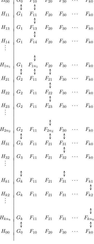
The schematic diagram in Table 1 indicates which adjunctions ofFij’s andGl’s

are involved with each of the adjunctions for the Hij’s. The vertical arrows

indicate individual adjunctions.

Table 1: Individual adjunctions forming composite multivariable adjunctions

H00 G0 F10 F20 F30 · · · Fk0

H11 G1 F11 F20 F30 · · · Fk0

H13 G1 F13 F20 F30 · · · Fk0

H14 G1 F14 F20 F30 · · · Fk0

.. .

H1n1 G1 F1n1 F20 F30 · · · Fk0

H21 G2 F11 F21 F30 · · · Fk0

H22 G2 F11 F22 F30 · · · Fk0

H23 G2 F11 F23 F30 · · · Fk0

.. .

H2n2 G2 F11 F2n2 F30 · · · Fk0

H31 G3 F11 F21 F31 · · · Fk0

H32 G3 F11 F21 F32 · · · Fk0

.. .

Hk1 Gk F11 F21 F31 · · · Fk1

Hk2 Gk F11 F21 F31 · · · Fk2

.. .

Hknk Gk F11 F21 F31 · · · Fknk

This is much easier to construct formally using Theorem 2.2: we just need to exhibit mutual left1-variable adjoints for each of the m functors obtained fromH00by fixing all but one of the variables. Now fixing every variable except aij in the functor

H11=G0(F10, . . . , Fk0)

we construct a mutual left adjoint using

the mutual left adjoint forFi0 with all but thejth variable fixed, and

the mutual left adjoint forG0 with all but theith variable fixed.

These compose to give the adjoint required. We can depict this schematically as follows. We depict the latter as

b1 · · · bi · · · bm

b0

so then composing this with the former looks like the diagram below, where

Fi0 and G0 are the multifunctors pointing downwards, and the 1-variable left

adjoint is indicated as the dotted arrow pointing upwards.

b1

· · · bi · · · bm

b0 G0

ai1

· · · aij· · ·aini

b0

Fi0

That is, starting from the functor

Fi0:Ai1× · · · ×Aini A

•

we fix all but the jth variable and have a mutual left adjoint, that is right adjoint for

F•

i0(ai1, . . . , ai,j−1, , ai,j+1, . . . , aini) :A

•

ij Ai0

which is

Fij(ai,j+1, . . . , aini, , ai1, . . . , ai,j−1) :Ai0 A

•

ij.

Also consider

G•

0(b1, . . . , bi−1, , bi+1, . . . , bk) :Bi• B0

with its right adjoint

Gi(bi+1, . . . , bk, , b1, . . . , bi−1) :B0 Bi•=Ai0.

Now we simply compose the functors

B0 Ai0 A•ij

setting each

bq=Fq0(aq1, . . . , aqnq).

Using the previous shorthand this is the composite

Fij , Gi(Fi+1,0, . . . , Fk0,•, F10, . . . , Fi0), .

This completes the construction of composition. Identities are given by identity adjunctions, which obviously satisfy unit conditions. Associativity follows from associativity of composition of n-variable functors (with one another) and of

1-variable adjunctions (with one another). 2

Special cases

1. If anyni= 0 this amounts to fixing the ith variable ofG. If all but 1 of

theni is 0 then we have fixed every variable except one, and if we do this

for eachni in turn we have effectively characterised the composite

multi-variable adjunction by producing the necessary 1-multi-variable adjunctions as in Theorem 2.2.

2. If we compose with the identity adjunction (as a 1-ary adjunction) for all but one of thei’s, we have effectively composed in just one position.

3. If we take everyni = 1 ork= 1 this says we can compose ann-variable

adjunction with 1-variable adjunctions (pre- or post-) to get a new n

2.4

Multivariable mates

We now give a multivariable version of the calculus of mates. As for the ad-junctions, we start with the 2-variable case and proceed inductively.

Proposition 2.11. Suppose we have two 2-variable left adjunctions of functors

F:A×B C• _{and F}′_:A′_×B′ _C′•

G:B×C A•

G′ : B′

×C′

A′•

H:C×A B•

H′ :C′

×A′

B′•

,

together with functors

S: A A′

T:B B′

U:C C′

and a natural transformation

A×B A′

×B′

C•

C′•

S×T

U•

F F′

α

with components

αa,b:F′(Sa, T b) U F(a, b).

Then for eachb∈B we have a natural transformation

A A′

C•

C′•

S

U•

F( , b) F′_{( , T b)} α ,b

with mate

C C′

A•

A′•

. U

S•

G(b, ) G′_{(T b, )} α ,b

Then in fact the components(α ,b)c are the components of a natural

transfor-mation

B×C B′

×C′

A•

A′•

. T×U

S•

G G′

¯

Dually if we start with 2-variablerightadjunctions then the result holds with all the natural transformations pointing in the opposite direction as below.

A×B A′_×B′

C•

C′•

S×T

U•

F α F′

Proof. We just need to check that the components ¯αb,c = (α ,b)c are natural

inb;a priori they are natural inc. We use the fact thatαis natural in b. As with Theorem 2.2 the proof is possible by a 1-dimensional diagram chase, but we provide a 2-categorical proof as it is quite aesthetically pleasing.

Now the natural transformationα ,bis given by the following composite

C B×C A•

A′•

A•_×B•

A′•

×B′•

B×C

C C′ _B′

×C′

A′•

b×1 G S•

S•×T•

U T b×1 G′

1×b•

F•

1×T b•

F′ •

1

1

b×1

T×U εb

η′ T b α•

taking care over the direction as the target is inA′•

. Again we use the fact that

a morphismb1 F b2in B corresponds to a natural transformation

1 f B

b1

b2

thus to check that the components

C A′•

B×C

B×C

b×1 S•_G

b×1 _G′_(T×U)

¯

αb,

are natural inb we show that for allb1

C A′•

B×C

B×C b1×1

b2×1

S•_G

b2×1 _G′_(T×U) ¯

αb, f×1

= _{C A}′•

. B×C

B×C b1×1 S•G

b1×1

b2×1

G′_(T×U)

¯

αb,

f×1

We have

C B×C A•

A′•

A•_×B•

A′•_×B′•

B×C

C C′ _B′_×C′

A′•

b1×1

b2×1

f×1 G S•

S•×T•

U T b2×1 G′

1×b• 2

F•

1×T b• 2

F′ •

1

1

b2×1

T×U εb2

η′ T b2 α•

=

C B×C A•

A′•

A•_×B•

A′•_×B′•

B×C

C C′ _B′_×C′

A′•

b1×1 G S•

S•_×T•

U T b2×1 G′

1×b• 2

1×b• 11×f

•

F•

1×T b• 2

F′ •

1

1

b2×1

T×U εb1

η′ T b2 α•

=

C B×C A•

A′•

A•_×B•

A′•_×B′•

B×C

C C′ _B′_×C′

A′•

b1×1 G S•

S•×T•

U T b2×1 G′

1×b• 1

F•

1×T b• 2

1×T b• 11×Tf

•

F′ •

1

1

b2×1

T×U εb1

=

C B×C A•

A′•

A•

×B•

A′•

×B′•

B×C

C C′ _B′

×C′

A′•

b1×1 G S•

S•_×T•

U

T b1×1

T b2×1 Tf×1

G′

1×b• 1

F•

1×T b• 1

F′ •

1

1

b2×1

T×U εb1

η′ T b1

α•

=

C B×C A•

A′•

A•

×B•

A′•

×B′•

B×C

C C′ _B′

×C′

A′•_.

b1×1 G S•

S•_×T•

U T b1×1 G′

1×b• 1

F•

1×T b• 1

F′ •

1

1

b1×1 b2×1

f×1

T×U εb1

η′ T b1

α•

2

Remark 2.12. Note that in the definition of the mate of α we could start by fixing the first variable instead of the second variable and then follow the analogous process to produce a natural transformation ˆαas below:

C×A C′_×A′

B•

B′•_.

U×S

T•

H H′

ˆ

α

Note that ¯αˆ=α= ˆα¯by the usual mates correspondence; the following result deals with a less trivial combination of these processes. This can be thought of as the 2-variable version of the mates correspondence.

Proposition 2.13. Given 2-variable adjunctions and a natural transformation

αas above,α¯¯ = ˆα.

Lemma 2.14(Generalised triangle identity). For a 2-variable adjunction, the following triangles commute, along with all cyclic variants.

H(F(a, b), a) b

H F(a, b), G(b, F(a, b)) ε

H(1, ε) ε

H(c, G(b, c)) b

H F(G(b, c), b), G(b, c) ε

H(ε,1) ε

Proof. This follows from the “cycle of isomorphisms” as in Example 2.6. 2

In the following proof we adopt notational shorthand as below, for simplifi-cation, clarity and to save space.

1. All objects have been omitted. The source categories can always be deter-mined from the functors shown, and whenever a variable inAis required, it is understood to bea; likewise forc∈C. For example:

T H meansT H(c, a), and

G(H,1) meansG(H(c, a), c)).

2. As in Remark 1.4 we write all units and counits for all adjunctions as

ε; the source and target functors uniquely determine which adjunction is being used, and the object at which the component is being taken.

For example, the above two triangles become:

H(F,1) 1

H(F, G(1, F))

ε

H(1, ε) ε

H(1, G) 1

H(F(G,1), G).

ε

H(ε,1) ε

Proof of Proposition 2.13. It suffices to show that these two natural transformations have the same component at (c, a)∈C×A. This is shown in the following (large) commutative diagram in which the top edge is the component ¯¯

αc,a and the bottom edge ˆαc,a.

Regions (3) and (4) are naturality squares, (5) and (6) are functorality ofH′_, (2) and (7) are generalised triangle identities and (1) commutes by extranatu-rality ofεas follows. The counitεin question has components

H′ (c, G′

(b, c)) b

and is natural inbbut extranatural inc. Region (1) is obtained by writing out the extranaturality condition for the morphism

F′

H′ (U, S)

H′_{(U, SG(H,1))}

H′ (U, G′

(T H, F′

(SG(H,1), T H)))

H′ (U, G′

(T H, U F(G(H,1), H)))

H′ (U, G′

(T H, U))

T H H′

(U, G′

(T H, F′

(S, T H)))

H′_{(U, G}′_{(T H, U F(1, H)))}

H′

(U F(1, H), G′

(T H, F′

(S, T H)))

H′ (F′

(S, T H), G′

(T H, F′

(S, T H)))

H′_{(1, Sε)}

H′_{(1, ε)}

H′_{(1, G}′_{(1, α))}

H′_{(1, G}′_{(1, U ε))}

ε

H′_{(U ε,1)} ε

H′_{(1, G}′_{(1, α))}

H′_{(1, G}′_{(1, U ε))}

H′_{(U ε,1)}

H′_(α,1)

ε H′_{(1, ε)}

H′_{(1, G}′_{(1, F}′_(Sε,1)))

H′_{(1, G}′_{(1, U F(ε,1)))}

H′_{(1, ε)}

H′_{(1, ε)}

1

2

3

4

5

6 7

2

Now by allowingB to be a finite product of categories, we get a notion of

n-variable mates with respect to ann-variable adjunction.

Theorem 2.15. Suppose we have functors

F0:A1× · · · ×An A•0, F′

0:A

′

1× · · · ×A

′

n A

′

0

•

equipped withn-variable left adjoints, and for all 0≤i≤n a functor

Si:Ai A′i.

Then a natural transformation

A1× · · · ×An A′1× · · · ×A′n

A•

0 A′0

•

S1× · · · ×Sn

S• 0

F0 F0′

α

has for all1≤i≤na mate

Ai+1× · · · ×Ai−1 A′i+1× · · · ×A′i−1

A•

i A′i

•

Si+1× · · · ×Si−1

S• i

Fi _α Fi′

i

given as in Proposition 2.11 with

A = Ai

B = A1× · · · ×Ai−1×Ai+1× · · · ×An C = A0.

We now give the n-variable version of the mates correspondence, which fol-lows from the 2-variable case (Proposition 2.13). First we need to fix our nota-tion carefully.

Notation for n-variable mates.

Suppose we have functors

F0:A1× · · · ×An A•0, F′

0:A

′

1× · · · ×A

′

n A

′

0

•

equipped withn-variable left adjoints, and for all 0≤i≤na functor

Then for any 0≤i≤n, given a natural transformationαas below

Ai+1× · · · ×Ai−1 A′i+1× · · · ×A′i−1

A•

i A′i

•

Si+1× · · · ×Si−1

S• i

Fi _α Fi′

and anyj6=iwe denote byαij the mate

Aj+1× · · · ×Aj−1 A′j+1× · · · ×A′j−1

A•

j A′j

•

Sj+1× · · · ×Sj−1

S• j

Fj Fj′

αij

produced by Theorem 2.15. Note that in this notation, the mate calledαi in

the theorem would be calledα0i.

Theorem 2.16(The n-variable mates correspondence). Given a pair of

n-variable adjunctions, any distinct i, j, k and a natural transformation α as above, we have

(αij)jk=αik.

Proof. Restricting to the functors Fi, Fj, Fk and fixing all variables except

those inAi, Aj, Ak we get a 2-variable adjunction. The result is then simply an

instance of Proposition 2.13 since it suffices to check it componentwise. 2

Corollary 2.17. Given a pair ofn-variable adjunctions as above and a natural transformation

A1× · · · ×An A′1× · · · ×A

′

n

A•

0 A′0

•

S1× · · · ×Sn

S• 0

F0 _α F0′

we have

((· · ·((α01)12)· · ·)n−1,n)n0=α.

That is, taking matesn+ 1times is the identity.

Note that then-variable mates correspondence respects horizontal and ver-tical composition. For horizontal composition this follows immediately from the analogous result for 1-variable mates. For vertical composition a little more effort is required, but mainly just to make precise the meaning of “respects ver-tical composition”. However this is only a matter of indices. The idea is not hard: composition of multivariable adjunctions is defined by fixing variables and composing the resulting 1-variable adjunctions, and the mates correspondence follows likewise.

3

Cyclic double multicategories

In this section we give the definition of “cyclic double multicategory”, the struc-ture into which multivariable adjunctions and mates organise themselves. The idea is to combine the notions of double category and cyclic multicategory so that in our motivating example the cyclic action expresses the multivariable mates correspondence.

Recall that a double category can be defined as a category object in Cat;

similarly a double multicategory is a category object in the category Mcatof

multicategories, and a cyclic double multicategory is a category object in the

categoryCMcat of “cyclic multicategories”. (Note that this could be called a

“double cyclic multicategory” but this might sound as if there are two cyclic actions.)

We build up to the definition step by step, with some examples.

3.1

Plain multicategories

We begin by recalling the definition of plain (non-symmetric) multicategories.

Definition 3.1. LetT be the free monoid monad on Set. WriteT-Spanfor the bicategory in which

0-cells are sets,

1-cellsA B areT-spans _X

T A B

s t

2-cells are maps ofT-spans.

Composition is by pullback using the multiplication forT: the composite

A X B Y C

is given by the span

.

T X Y

T B T2_A

T A

C µA

Amulticategory Ais a monad inT-Span, thus

aT-span _A1

T A0 A0

s t

equipped with unit and multiplication 2-cells. Explicitly, this gives

a setA0 of objects,

for all n ≥ 0 and objects a1, . . . , an, a0 ∈ A0 a set A(a1, . . . , an;a0) of n-ary “multimaps” (in the casen= 0 the source is empty)

equipped with

composition: for all sets ofk ordered stringsai1, . . . , aimi, ai0 and a00 in

A0 a function

A(a10, . . . , ak0;a00)×A(a1;a10)× · · · ×A(ak;ak0) A(a1, . . . , ak;a00)

where we have writtenai for the stringai1, . . . , aini, and

identities: for alla∈A0 a function

1 1a

A(a;a)

satisfying the usual associativity and unit axioms.

Note that we can define composition at the ith input by composing with

identities at every other input; this will be useful when giving the axioms for a cyclic multicategory and we denote it◦i.

Examples 3.2.

1. Multifunctors: take objects to be categories and k-ary multimaps to be

multifunctors, that is functors of the form

A1× · · · ×Ak A0.

2. Multicategories from monoidal categories: given any monoidal categoryC

there is a multicategoryMC with the same objects, and with

MC(x1, . . . , xk;x0) =C(x1⊗ · · · ⊗xk, x0).

3. Profunctors: we might try to use profunctors instead of functors in the above example, but this would form some sort of “weak multicategory” or “multi-bicategory” as profunctor composition is not strictly associative and unital. However this is a pertinent case to consider. A profunctor

is by definition a functor

A1× · · · ×Ak×A•0 Set.

But this also gives rise to a profunctor ˆ

Ai×A•0 A

•

i

for each i6= 0 where here ˆAi denotes the product A1× · · ·Ai−1×Ai+1× · · · ×Ak.

Strictness aside, this is the sort of cyclic action we will be considering. (In fact, the cyclic action in this example is strict although the composition is not.)

3.2

Cyclic multicategories

We now introduce the notion of a “cyclic action” on a multicategory. Symmetric multicategories are multicategories with a symmetric group action that can be thought of as permuting the source elements of a given multimap. Cyclic multicategories have acyclicgroup action that permutes the inputsandoutputs cyclically. There is also a “duality” that is invoked each time an object moves between the input and output sides of a map under the cyclic action, as in the example with profunctors sketched above.

Throughout, we work with Cn the cyclic group of order n considered as a

subgroup of the symmetric groupSn with canonical generator the cycle σn =

(123· · ·n). We will often write this asσ with its order being understood from the context.

Definition 3.3. Acyclic multicategoryX is a multicategory equipped with

an involution on objects

X0 X0

x x∗

for everyn≥1 and ordered stringx0, x1, . . . , xn an isomorphism σ=σn+1:X(x1,· · ·, xn;x0)

∼

X(x2, . . . , xn, x∗0;x

∗

1)

such that the following axioms are satisfied.

1. Each isomorphismσn is cyclic so that (σn)n = 1.

2. The identity is preserved byσ2, that is, the following diagram commutes

1 X(x;x)

X(x∗ ;x∗

)

1x

3. Interaction betweenσand composition.

Letci denote composition at theith input only, that is

ci:X(y1, . . . , ym;y0)×X(x1, . . . , xn;yi) X(y1, . . . , yi−1, x1, . . . , xn, yi+1, . . . , ym;y0)

Then the following diagrams commute.

Fori= 1, that is, for composition at the first input:

X(y1, . . . , ym;y0)×X(x1, . . . , xn;y1) X(x1, . . . , xn, y2, . . . , ym;y0)

X(y2, . . . , ym, y0∗;y

∗

1)×X(x2, . . . , xn, y∗1;x

∗

1)

X(x2, . . . , xn, y∗1;x

∗

1)×X(y2, . . . , ym, y0∗;y

∗

1) X(x2, . . . , xn, y2, . . . , ym, y∗0;x

∗

1).

c1

cn σ×σ

∼

=

σ

Ifi6= 1

X(y1, . . . , ym;y0)×X(x1, . . . , xn;yi) X(y1, . . . , yi−1, x1, . . . , xn, yi+1, . . . , ym;y0)

X(y2, . . . , ym, y0∗;y

∗

1)×X(x1, . . . , xn;yi) X(y2, . . . , yi−1, x1, . . . , xn, yi+1, . . . , ym, y0∗;y

∗

1).

ci

ci−1

σ×1 σ

In algebra

σ(g◦if) = (

(σf)◦n(σg) i= 1

(σg)◦i−1f 2≤i≤m.

We can depict the axioms (3) pictorially as follows. Depictingf ∈X(x1, . . . , xn;x∗0)

as

x1 x2 xn

x∗

0 f

we depictσf as

x1 x2 · · · xn

f

x∗

0 x∗

1

x0

Then the first axiom is depicted as shown below.

x1 x2 · · · xn

f

y1 y2 · · · ym

g

y∗

0 x∗

1

y0

= x1 x2 · · · xn

f

y1 x∗

1

y∗

1

y1 y2 · · · ym

g

y∗

0 y∗

1

y0

below.

=

x1 x2 · · · xn

f

y1 · · · yi· · ·ym

g

y∗

0 y∗

1

y0

x1 x2 · · · xn

f

y1 · · · yi· · ·ym

g

y∗

0 y∗

1

y0

Note that these two axioms are equivalent to a single axiom involving the cyclic action and composition at every variable.

Examples 3.4. First we give some slightly degenerate examples.

1. IfX is a cyclic multicategory with only one object (so the involution must be the identity) then we have a notion of non-symmetric cyclic operad as given by Batanin and Berger in [1]. This is in contrast to the definition of (symmetric) cyclic operad in [14].

2. More generally, the involution can be the identity even for a non-trivial set of objects.

Example 3.5. We define a cyclic multicategoryMAdjas follows. Take objects to be categories, and a multimap

A1, . . . , An A0

to be a functor

A1× · · · ×An F0

A0

equipped with alln-variable left adjoints,F1, . . . , Fn. The involution ()∗is then

given by ()•

and the cyclic action is given by

σ:Fi Fi+1

and the axioms are satisfied by construction. We could also do this with n

-variable right adjoints.

Note thatMAdjcan be expressed using profunctors. Recall our profunctor

example that was not quite a true example (Example 3.2.3) as profunctor com-position is not strictly associative or unital; nevertheless it has a strict cyclic action. In factn-variable adjunctions can be thought of asn-variable profunc-tors F0 such that F0 and all its cyclic versions in Prof are representable, or,

Proposition 3.6. LetP :A1× · · · ×An×A0 Setbe a profunctor equipped

with a representation for eachP(a1, . . . , ai−1, , ai+1, . . . , an, a0). That is, given

ai+1, . . . , ai−1

an objectFi(ai+1, . . . , ai−1)∈Ai and an isomorphism

P(a1, . . . , a0)∼=Ai(Fi(ai+1, . . . , ai−1), ai) (4)

natural inai.

Then the Fi canonically extend to functors

Ai+1× · · · ×Ai−1

Fi

A•

i

forming ann-variable (left) adjunction.

Proof. By standard results about parametrised representability, each Fi

ex-tends to a functor

Ai+1× · · · ×Ai−1

Fi

A•

i

unique making the isomorphism (4) above natural in all variables. For the

n-variable adjunction we then compose the isomorphisms

Aj(Fj(aj+1, . . . , aj−1), aj)

∼

=

P(a1, . . . , a0)

∼

=

Ai(Fi(ai+1, . . . , ai−1), ai).

2

Remark 3.7. Note that composition of these profunctors matches composi-tion of the corresponding multivariable adjunccomposi-tions up to isomorphism; this is as strict as we can expect as profunctor composition is only defined up to isomorphism (by coends).

Remark 3.8. The idea is that we consider the functor

Cat Prof

that is the identity on objects and on morphisms sends a functor

A G B

to the profunctor

A B

given by

A×B•

Set (a, b) B(b, Ga).

With the usual composition inProfthis is only a pseudo-functor, giving us a

“sub-pseudo-multicategory” of Prof that is somehow “equivalent” to MAdj.

3.3

Cyclic double multicategories

We are now ready to introduce the 2-cells we need. Recall that a double category can be defined very succinctly as a category object in the category of (small) categories. We proceed analogously for the multi-versions.

Definition 3.9. Adouble multicategoryis a category object in the category

Mcatof multicategories.

Acyclic double multicategoryis a category object in the categoryCMcat of cyclic multicategories.

Note that pullbacks in the categoryCMcatare defined in the obvious way,

so this definition makes sense. As with double categories, it is desirable to give

an elementary description. A cyclic double multicategoryX has as underlying

data a diagram

B s A

t

inCMcat.

Recall that the underlying data for a multicategoryA is in turn a diagram

in sets of the following form

A1

T A0 A0

d c

whereT is the free monoid monad onSet. Thus for a category object inMcat

we have a diagram of the following form inSet:

B1

T B0 B0 A1

T A0 A0

d c

d c

t s

t s t

s

where the sets correspond to data as follows:

A0 = 0-cells

A1 = vertical (multi) 1-cells

B0 = horizontal (plain) 1-cells

Commuting conditions tell us that 2-cells might be depicted as:

x1 x2

xn

x•

0 f

· · · ·

y1 y2

yn

y•

0 g s1

s2

sn

s• 0 α

Inside the structure of a (cyclic) double multicategory we have two categories given by

0-cells, horizontal 1-cells and horizontal composition, and

vertical 1-cells, 2-cells and horizontal composition

and two (cyclic) multicategories with objects and multimaps given by

0-cells, vertical 1-cells and vertical multi-composition, and

horizontal 1-cells, 2-cells and vertical multi-composition.

Furthermore these must all be compatible, in the following sense. In addition to the underlying diagram

B s A

t

inCMcatwe must have an identity map

I:A B

and a composition map

γ:B×AB B

ands, t, I, γmust all be maps of cyclic multicategories, that is, they must respect (co)domains, composition, involution and cyclic actions in passing fromBtoA. Note thats/tgive “horizontal source and target”,Igives “horizontal identities”

and γ “horizontal composition”. Respecting (co)domains and composition is

analogous to the axioms for a double category, just with multimaps instead of 1-ary maps where appropriate; notably this gives us interchange between horizontal and vertical composition.

Respecting involution and cyclic actions gives us the following information.

1. Horizontal source and target respect involution: we have an involution on

A0(0-cells) and an involution onB0(horizontal 1-cells), both written ( )∗

under which

x f y x∗ f∗

y∗