This is a repository copy of
The optimisation of stochastic grammars to enable
cost-effective probabilistic structural testing
.
White Rose Research Online URL for this paper:
http://eprints.whiterose.ac.uk/132851/
Version: Accepted Version
Article:
Poulding, S., Alexander, R. orcid.org/0000-0003-3818-0310, Clark, J.A.
orcid.org/0000-0002-9230-9739 et al. (1 more author) (2015) The optimisation of
stochastic grammars to enable cost-effective probabilistic structural testing. Journal of
Systems and Software. pp. 296-310. ISSN 0164-1212
https://doi.org/10.1016/j.jss.2014.11.042
[email protected] Reuse
This article is distributed under the terms of the Creative Commons Attribution-NonCommercial-NoDerivs (CC BY-NC-ND) licence. This licence only allows you to download this work and share it with others as long as you credit the authors, but you can’t change the article in any way or use it commercially. More
information and the full terms of the licence here: https://creativecommons.org/licenses/
Takedown
If you consider content in White Rose Research Online to be in breach of UK law, please notify us by
The Optimisation of Stochastic Grammars to Enable
Cost-Effective Probabilistic Structural Testing
S. Pouldinga,b,∗
, R. Alexanderb, J.A. Clarkb, M.J. Hadleyb
a
Blekinge Institute of Technology, 371 79 Karlskrona, Sweden
b
University of York, Heslington, York, YO10 5DD, United Kingdom
Abstract
The effectiveness of statistical testing, a probabilistic structural testing strategy, depends on the characteristics of the probability distribution from which test inputs are sampled. Metaheuristic search has been shown to be a practical method of optimising the characteristics of such distributions. However, the applicability of the existing search-based algorithm is limited by the requirement that the software’s inputs must be a fixed number of ordinal values.
In this paper we propose a new algorithm that relaxes this limitation and so permits the derivation of probability distributions for a much wider range of software. The representation used by the new algorithm is based on a stochastic grammar supplemented with two novel features: conditional production weights and the dynamic partitioning of ordinal ranges. We demonstrate empirically that a search algorithm using this representation can optimise probability distri-butions over complex input domains and thereby enable cost-effective statistical testing, and that the use of both conditional production weights and dynamic partitioning can be beneficial to the search process.
Keywords:
search-based software engineering, software testing, statistical testing, probabilistic structural testing, grammar-based testing
1. Introduction
Probabilistic testing strategies generate test inputs by random sampling from an input profile: a probability distribution over the input domain of the software-under-test (SUT). The most straightforward probabilistic strategy is uniform random testing in which test inputs are sampled from a uniform distribution, i.e. one in which all possible inputs for the SUT have the same chance of be-ing selected. Generatbe-ing test data usbe-ing uniform random testbe-ing requires only
∗Corresponding author
Email addresses: [email protected](S. Poulding),[email protected]
(R. Alexander),[email protected](J.A. Clark),[email protected](M.J. Hadley)
*Manuscript
knowledge of the bounds on the input domain; other information about the SUT, such as the source code structure or the software’s functionality, is not required. Thus applying uniform random testing to most software is relatively simple and the data generation process has little overhead.
The ease of data generation for uniform random testing is often a trade-off with the poorer fault-detecting efficiency of the strategy: for some (though not necessarily all) software larger test sets may be required to detect as many faults as deterministic techniques such as partition testing (Duran and Ntafos, 1984; Boland et al., 2003). When the cost of running each test case is expensive, for example because executing the software with the test case is time-consuming or checking the correctness of the output requires a manual oracle such as a human domain expert, the larger test sets required of uniform random testing would significantly increase the overall testing costs.
In the 1990s, Th´evenod-Fosse and Waeselynck described a more sophisti-cated probabilistic testing strategy calledstatistical testingwhich, by using more information about the SUT, has better fault-detecting efficiency (Th´evenod-Fosse and Waeselynck, 1991, 1993; Th´evenod-(Th´evenod-Fosse et al., 1995). Statistical testing uses an input profile specifically tailored to the SUT so that all mem-bers in a chosen set of coverage elements—typically structural elements such as branches in the source code or functional elements based on the specification— have a high chance of being exercised by a test input sampled from the input profile. Th´evenod-Fosse and Waeselynck showed that when this adequacy crite-rion is satisfied, statistical testing often detects more faults than uniform random testing using test sets of the same size.
Having derived a SUT-specific profile for statistical testing, the test data gen-eration process is as straightforward as random testing. However, it can be very difficult to derive the SUT-specific profile for software of realistic size: existing approaches are either manual, and therefore expensive if they are tractable at all (Th´evenod-Fosse et al., 1995), or semi-automated model-based approaches that are limited in their applicability and which scale poorly (Gouraud et al., 2001). It is this problem that motivates our investigation of automated search-based algorithms that can cheaply derive SUT-specific input profiles for use in statistical testing: by reducing the cost of deriving the profile, the potential fault-detecting efficiency of statistical testing may then be realised.
We described one such search-based algorithm in our previous work (Pould-ing and Clark, 2010; Pould(Pould-ing et al., 2011). The algorithm represented input profiles as a Bayesian network in which each node corresponded to one input argument. The algorithm, while otherwise effective, was restricted by this repre-sentation to software whose inputs were a fixed number of arguments that each had a numeric (or other ordinal) data type—for example, a function with two integer arguments. This limited the applicability of the algorithm since many SUTs have inputs that are more complex than this.
which the inputs vary in size—for example, variable-length sequences, strings, or arrays—and in which the inputs may have data types other than ordinal, including data types that must satisfy complex constraints on their structure— for example, data formatted as XML or JSON. We demonstrate how the new algorithm can be applied to three real-world SUTs that have complex input domains with these characteristics.
The grammar-based representation used by the algorithm incorporates two novel features: conditional production weights that permit a limited form of context-sensitivity, and dynamic partitioning of grammar variables that repre-sent ordinal data types. We hypothesise that these extensions facilitate the derivation of input profiles by the algorithm and thus further reduce the cost. The second contribution of the paper is a rigorous empirical assessment of the effect of these two features on algorithm, both singly and in combination, in order to test this hypothesis.
The paper is structured as follows. In section 2 we explain the technique of statistical testing, and outline the algorithm using the Bayesian network representation from our previous work. The new algorithm using the grammar-based representation is described in section 3. An empirical demonstration of the algorithm and an evaluation of the novel extensions to the representation are presented in section 4. In section 5, we discuss our proposed algorithm in relation to other methods for deriving input profiles, and summarise our conclusions in section 6.
2. Background
2.1. Statistical Testing
Statistical testing requires that the input profile for the particular software-under-test (SUT) satisfies an adequacy criterion. The criterion is expressed in terms of a set,C, of coverage elements such as structural elements of the SUT’s source code or functional elements of the SUT’s specification. For each coverage element,ci ∈ C, letpi be the probability that the coverage element is exercised by a single input chosen at random from the given input profile, and pmin be
the minimum of the set{pi}. We will refer to pmin as theminimum coverage
probability. The adequacy criterion is that the minimum coverage probability should be above a suitably high target value.
The rationale for this criterion is efficient coverage of the structural elements. LetQi be the probability that the coverage element ci is exercised by at least one test case in a test set of size N, and Qmin be the minimum of the set
{Qi}. Adapting a result given by Th´evenod-Fosse and Waeselynck (1993), the relationship betweenQmin,pmin, and N is given by:
Qmin= 1−(1−pmin)N (1)
For effective testing, Qmin should have a value close as possible to 1 so that it
test set size (which might improve the fault-detecting ability); or a reduction in the test size (and thus the testing costs) while maintaining an acceptable value ofQmin.
A number of techniques have been proposed for deriving input profiles that satisfy the adequacy criterion. Gouraud et al. (2001) describe a static technique which assigns weights to edges in the SUT’s control-flow graph in order to sam-ple execution paths in a manner that satisfies the adequacy criterion. However, computationally expensive constraint-solving is required to derive test inputs which exercise the sampled paths, and many of sampled paths are unfeasible in practice. Both these factors limit the scalability of the technique. Th´evenod-Fosse et al. (1995) describe a dynamic technique. The minimum coverage prob-ability of a candidate input profile is estimated by executing an instrumented version of the SUT with inputs sampled from the profile. The results are used to guide the manual adjustment of the profile, and the process repeated until a suitable value of the minimum coverage probability is attained. However, Th´evenod-Fosse et al. speculate that this technique is unlikely to be practical for large SUTs in its manual form. The lack of scalability inherent in both these techniques motivates the use of an automated search-based algorithm for deriving input profiles.
2.2. Deriving Input Profiles Using Search
We have previously demonstrated that metaheuristic search can automate the dynamic profile-derivation technique of Th´evenod-Fosse et al., and thereby reduce the cost of deriving suitable input profiles for statistical testing (Poulding and Clark, 2010).
In this earlier work, an assumption was made that inputs to the SUT were a fixed number of numeric (or other ordinal data type) arguments. This as-sumption enabled input profiles to be represented as Bayesian networks: di-rected acyclic graphs in which nodes correspond to input arguments, and edges describe conditional dependence between arguments. The conditional distribu-tions at each node were represented by partitioning the domain of the corre-sponding argument into a number of intervals and assigning a probability to each interval. To derive input profiles using this Bayesian network represen-tation, random mutation hill-climbing was used to optimise the edges between nodes, the number and size of intervals at a node, and the probabilities assigned to each interval.
In subsequent work, we demonstrated an enhancement to the search algo-rithm that improved performance by a factor of five for some SUTs (Poulding et al., 2011). The enhancement—which we called ‘directed mutation’—used ad-ditional information obtained from executing the instrumented SUT to bias the mutation operators to parts of the candidate input profile that exercised the coverage element(s) having the lowest coverage probability.
ap-proach may be applied. It is this limitation we seek to remove using the new grammar-based reprentation described in this paper.
3. Proposed Search Algorithm
In this section we describe the three components of the proposed search algorithm: the representation, the fitness metric, and the search method.
3.1. Representation
3.1.1. Stochastic Context-Free Grammars
Formal grammars define a language ofstrings: sequences of symbols drawn from a set of terminal symbols. The grammar restricts valid strings to be a subset of all the possible sequences of terminals by means of production rules: only those strings that can be constructed by the application of the grammar’s production rules are valid. The productions of context-free grammars, on which our representation is based, have the form:
V → X1 X2 ...Xn
where Vis one of an additional set of symbols called variables, and theXi are either variable symbols or terminals.
The generation of a valid string from the grammar begins with a string consisting of a single copy of the designated ‘starting’ variable symbol, usually denotedS. Generation proceeds by considering the leftmost variable in the cur-rent string. A production is chosen which has this variable on the left-hand side, and the variable is replaced in the string with the symbols on the right-hand side of the production rule. The process of replacing variables continues until the string contains no variable symbols.
As an example, consider the following context-free grammar for defining simple arithmetic expressions. (For clarity, we surround terminal symbols in this and subsequent grammars by single quotes. We also use the standard notation of concatenating productions with same left-hand side variable, separating the alternative right-hand sides using vertical bars: X → Y | Zis equivalent to the two productionsX → YandX → Z.)
S → Expr
Expr → Num | Expr Op Expr
Num → ‘0’ | ‘1’ | ‘2’ | ‘3’ | ‘4’ | ‘5’ Op → ‘+’ | ‘-’ | ‘*’ | ‘/’
This grammar generates valid strings such as‘4 + 3 * 5’, but does not gen-erate invalid strings such as‘- * 3 /’.
In a stochastic context-free grammar (SCFG), each production is addition-ally annotated by a weight. During string generation, if more than one produc-tion could be applied, the weights are interpreted as a probability distribuproduc-tion and one of the productions is chosen at random according to this distribution.
probability distribution over the inputs. (We note, however, that some types of input structures cannot be represented using context-free grammars.)
3.1.2. Conditional Production Weights
Context-free grammars are so-called because the set of productions that may be applied to a variable does not depend on the symbols occurring before or after the variable in the string during the generation process; this is a consequence of only a single variable being permitted on the left-hand side of production rules. The context-free property simplifies the grammar representation, but limits the types of input profiles that may be represented using the weights of a SCFG. Consider again the example grammar for generating simple arithmetic expres-sions. If an optimal input profile must avoid too many divide-by-zero arithmetic operations (i.e. the substring‘/ 0’), the only mechanism available to do this is to assign a low weight to the productionOp → ‘/’, or to the production Num → ‘0’. However such weights would also reduce the probability of otherwise desirable substrings such as‘/ 2’and‘+ 0’.
To overcome this limitation, we enhance the standard form of SCFGs by introducing conditional weights for the productions. A ‘child’ variable may be identified as having one or more ‘parent’ variables (the set of which may include the child variable itself) on which it is dependent. The distribution of weights over the productions for the child variable is then conditionally dependent on which of the parent variables’ productions were most recently applied.
For example, the variable Numin our example grammar may be dependent on the variable Op. The weights over the 6 productions for Numare then con-ditionally dependent on which production was most recently applied toOp. In effect, there are 5 (potentially different) distributions of weights over the pro-ductions of Num: one for each of the 4 possible productions of Op, plus a further distribution that is used if no production has yet been applied toOp.
The conditional dependency of weights extends the types of input profiles that may be represented by introducing a limited form of context-sensitivity (but only in the weights; the grammar itself remains context-free). It would, for example, enable divide-by-zero errors to be avoided more accurately by setting the weight ofNum → ‘0’to a low valueonlyin the conditional distribution used when the most recent production applied toOpwasOp → ‘/’, but retaining a normal weight forNum → ‘0’for all the other productions of Op.
The conditional dependency between variables—which parents are related to which child variables—is discovered by the search algorithm; it does not need to be specifieda priori.
3.1.3. Dynamic Partioning of Ordinal Ranges
productions and associated weights: it would be impractical to optimise such a large representation using search. An alternative could be to simply sample a value from the range using a fixed probability distribution, e.g. a uniform distribution, but such an arbitrary distribution may not result in an effective input profile.
Our proposed solution is to partition the variable’s range into a small number of intervals that we term ‘bins’, and create a production rule for each bin. Since each production has a (potentially conditional) weight assigned to it, a number of different probability distribution over the variable’s range can be represented. Moreover, the search algorithm can modify the production weights in order to find a suitable distribution. The representation is therefore more expressive and flexible than a fixed arbitrary choice such as a uniform distribution. We refer to variables represented in this way as ‘partitioned variables’.
For example, if the variableNumin the arithmetic expression grammar had a much larger range of [−32768,32767], it might be partitioned into three bins, and three production rules, as follows:
Num → [−32768,−2480] | [−2479,238] | [239,32767]
When one of these three productions is chosen during the generation of a string from the grammar, the output is not the bin, but a value picked at random from a uniform distribution across the bin. For example, if the production Num → [−2479,238] is applied, then the output is a single integer between -2479 and 238 chosen at random.
The number of bins, and the boundaries between bins, are dynamic: both of these aspects can be modified by the search algorithm. Thus, the number and lengths of bins need not specifieda priori: the search algorithm attempts to derive a suitable partitioning.
We note that this partitioning into bins is different, both in purpose and construction, from partition testing strategies, such as the approach of Richard-son and Clarke (1981). Firstly, the partition used for partition testing consists of equivalence classes in the context of functional or structural coverage; in the algorithm proposed in this paper, the partition is used to define a histogram probability distribution over the ordinal input argument that the grammar vari-able represents. It is possible that the bins derived by the algorithm may align with structural equivalence classes since inputs in the same class would be sam-pled with the same probability by the optimal profile for statistical testing, but there is no requirement that they do. Secondly, partition testing approaches typically identify partitions by static analysis; in this algorithm the partition is dynamically derived during the search process.
3.2. Fitness Metric
one (or more) times. The lowest value ofpi across all the coverage elements is an estimate of the minimum coverage probability. Therefore the fitness metric, f, is given by:
f = min ci∈C
1 K
K
j=1
ei;j
(2)
whereC is the set of coverage elements; andei;j is an indicator variable set to 1 if thejth execution of the SUT exercised coverage elementc
i, and 0 otherwise. Since the sample of inputs is of finite size, the fitness metric is only an approximation of the minimum coverage probability and may sometimes be higher than the ‘true’ value for the candidate input profile. In this situation, the input profile may in effect form an artificial local optimum and be retained in error over many iterations of the search. In our previous work, we were able to minimise this effect by continuing to evaluate the current input profile (for up toµevalhill-climbing iterations), and re-calculating a more accurate estimate
of the fitness from the accumulated instrumentation data (Poulding and Clark, 2010; Poulding, 2013).
3.3. Search Method
There is some correspondence between the new grammar-based represen-tation and the previous Bayesian network represenrepresen-tation. For this reason, we propose a hill-climbing search similar to that used in our earlier work (Poulding et al., 2011), and reinterpret the beneficial features of that search method in the context of the new grammar-based representation.
3.3.1. Random Mutation Hill-Climbing
The search begins from a random input profile constructed by choosing pro-duction weights, conditional dependencies between variables, and the number and size of bins for partitioned variables at random. The algorithm parameters specify upper limits for the number of parent variables on which any one vari-able may be conditionally dependent (µprnt), and for the number of bins that
a partitioned variable may have (µbins): both the initial random profile and
neighbours created by mutation respect these limits.
At each iteration of the hill-climb, a small number, λ, of neighbours to the current input profile are created by applying one of the following mutation operators:
Mprb increases or decreases a single production weight by a factorρprb;
Madd adds a conditional dependency between two grammar variables;
Mrem removes a conditional dependency;
Mlen increases or decreases the length of one bin of a partitioned variable by a
factorρlen;
Mjoi joins two adjacent bins.
The mutation operators were chosen to enable the search to make small changes to the weights of the stochastic grammar (Mprb, Madd, Mrem) and to
the bins of ordinal variables (Mlen,Mspl,Mjoi), and thereby permit the
deriva-tion of an optimal probability distribuderiva-tion over the grammar and partideriva-tioning of ordinal input arguments, respectively. For each mutation operator there is a corresponding operator that reverses its action (e.g. Madd and Mrem; Mprb
reverses itself when increasing the weight by the factor rather than decreasing, and vice versa) in order to ensure that all parts of the search space are reach-able from any other. We note that these are not the only mutation operators that could be used: for example, rather than mutating a production weight by multiplying it by a constant (operator Mprb), a constant could be added (or
subtracted) from the weight. However similar operators to these were found to be effective for the older algorithm that used a Bayesian network representation (Poulding, 2013).
Each mutation operator Mx has an associated weight, wx: operators with
higher weights are more likely to be applied when creating a neighbour. The neighbours are evaluated, and if the fittest neighbour is fitter than the current input profile, the neighbour becomes the current profile in the next iteration.
3.3.2. Directed Mutation
We incorporate an enhancement to the search method that we describe as ‘directed mutation’. This enhancement was discussed in section 2.2 above, and is explained in detail in our previous work (Poulding et al., 2011). When the fitness of the current input profile is evaluated, data is maintained as to which productions gave rise to inputs that exercised the coverage element(s) with the minimum coverage probability. The weights (and bins, if a partitioned variable) associated with these productions are then mutated with a higher likelihood when creating neighbours of the current input profile.
Directed mutation is implemented by grouping the mutation operators into three groups:
Gedge operators that modify conditional dependencies: Madd andMrem;
Gbins operators that modify production weights and bins directly: Mlen,Mspl,
Mjoi, andMprb;
Gdrct consists of the same weight- and bin-modifying operators as Gbins, but
applies themonlyto production weights and bins that contributed strings that exercised the coverage element(s) with the lowest coverage probabil-ity.
Each groupGx has associated weightWx. When choosing a mutation
the mutation operator weights. The group weights thus control the ‘strength’ of directed mutation effect.
If the minimum coverage probability is zero, one or more coverage elements must not have been exercised by any of the sampled inputs and so there is no data available with which to apply directed mutation. In this situation, the algorithm foregoes the local mutation operators described above and constructs entirely random neighbours in the same way as the initial random profile. The objective is to ‘jump’ directly to a new random point in the search space in the hope that the minimum coverage probability is non-zero around this new point and thus directed mutation will be effective.
4. Empirical Demonstration
4.1. Objective
The objective of the empirical demonstration described in this section is to evaluate the following propositions:
Proposition 1 The proposed search algorithm is able to derive effective input profiles for testing software that takes complex inputs. In this context, we define ‘complex’ to mean inputs that vary in length or which include data with types other than ordinal, including data types that must satisfy constraints on the structure of the test data. We contrast such inputs with the relatively simple input domains—a fixed number of numeric (or other ordinal) data types—that could be accommodated by the algorithm described in our previous work (Poulding and Clark, 2010; Poulding et al., 2011). Our measure of the efficacy is the minimum coverage probability of the input profile: the higher this probability, the smaller the test set required to exercise all of the chosen coverage elements. We cannot know the optimal minimum coverage probability for the SUTs considered in this work—the software is too complex to permit such a static analysis—and so instead we assess the efficacy of an input profile derived by the proposed algorithm by comparison with the best profile that can be derived by a random search using equivalent computational resources. Such a compar-ison will also verify that the problem is sufficiently difficult that a simple search algorithm such as random search is ineffective, and so the more sophisticated search algorithm proposed in this paper is required. (As a point of clarification, we note that the random search algorithm, in which profiles are sampled at random from the entire search space, is not the same as uniform random testing.)
4.2. Software-Under-Test
We use the following four SUTs as representative examples of software to which the algorithm could be applied. The first three SUTs—epuck,replace, circBuff—take ‘complex’ inputs that could not be represented by the Bayesian network used by the older algorithm. In all cases, the inputs are variable-length sequences consisting of both categorical and ordinal data types, and there are constraints on the valid ordering of the data within the sequence. The input domain of the fourth SUT—tcas—could be represented by a Bayesian network since its inputs consist of twelve numeric arguments, and is included here to demonstrate that the new algorithm is also practical for such SUTs.
The algorithm requires a context-free grammar that defines valid inputs to the software, and so in the following description of each SUT we also describe a grammar that specifies valid inputs. For software taking ‘complex’ inputs of this type, any automated test data generation method including random testing would require a grammar (or equivalent formal specification) if it is to generate valid inputs. We note, however, that the construction of such a grammar, if it does not already exist, does add to the cost of applying the algorithm proposed by this paper.
Ideally we would have used a larger number of example SUTs in order that we may more confidently generalise the empirical results to other software. In addition, a larger set of SUTs would have reduced the potential for overfitting the parameter settings that we tune for each algorithm variant (see section 4.5); the risk of such overfitting is discussed in (Arcuri and Fraser, 2011). However, we are constrained by the computing resources available: a large number of trials are performed in order to set algorithm parameters in a principled manner and to ensure a reliable assessment of performance given that the stochastic nature of the algorithm. Additional example SUTs would have further increased the number of trials, and thus computing resources, required for the empirical work. The instrumented version of each of the SUTs is available at: http://www. cs.york.ac.uk/~smp/supplemental/.
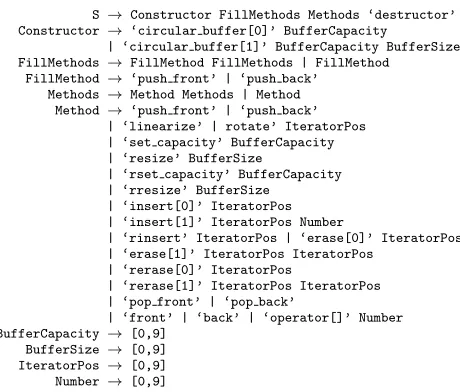
4.2.1. SUT: circBuff
circBuffis the implementation of a circular buffer container in the BOOST C++ library, version 1.50. The testing objective is coverage of all branches in the public methods of the public interface class of the container. (We omit the copy constructor and assignment operator in order to avoid a step-change in the complexity of the grammar since these methods take a further container object as a parameter.) The number of branches to be covered is 78. The public methods of the class constitute approximately 700 lines of code, but not all methods include branched code.
S→Constructor FillMethods Methods ‘destructor’ Constructor →‘circular buffer[0]’ BufferCapacity
| ‘circular buffer[1]’ BufferCapacity BufferSize FillMethods →FillMethod FillMethods | FillMethod
FillMethod→‘push front’ | ‘push back’ Methods →Method Methods | Method
Method →‘push front’ | ‘push back’ | ‘linearize’ | rotate’ IteratorPos | ‘set capacity’ BufferCapacity | ‘resize’ BufferSize
| ‘rset capacity’ BufferCapacity | ‘rresize’ BufferSize
| ‘insert[0]’ IteratorPos | ‘insert[1]’ IteratorPos Number
| ‘rinsert’ IteratorPos | ‘erase[0]’ IteratorPos | ‘erase[1]’ IteratorPos IteratorPos
| ‘rerase[0]’ IteratorPos
| ‘rerase[1]’ IteratorPos IteratorPos | ‘pop front’ | ‘pop back’
| ‘front’ | ‘back’ | ‘operator[]’ Number BufferCapacity →[0,9]
BufferSize→[0,9] IteratorPos →[0,9] Number →[0,9]
Figure 1: The grammar defining inputs tocircBuff
that fill the buffer, method calls that operate on the buffer, and finally a call to the destructor. Terminals, such as‘push front’, specify method calls. (The suffixes of the form[n]distinguish between overloaded methods.) Parameters to method calls are represented by the four partitioned variables at the end of the grammar. Recursion in the grammar enables the generation of variable-length sequences of method calls.
It is possible that one extremely long sequence of method calls could cover most, if not all, branches in a single test case. However, such a test case may be impractical in terms of applying an oracle, i.e. checking that the observed behaviour of the SUT is correct. We therefore place a pragmatic upper limit of 64 symbols on strings sampled from the grammar (as well as on intermediate strings during the sampling process)1.
The strings generated by the grammar are interpreted by a test harness and applied to an instrumented version of the container class. The object returned by a call to a constructor method is stored by the harness and subsequent method calls are made to that object.
4.2.2. SUT: epuck
‘E-pucks’ are small, relatively cheap robots used in robotics research. The SUTepuck is controller code that forms part of a lightweight simulator for e-puck robots written in C by Paul O’Dowd of the University of Bristol. Features supported by the simulator include infra-red proximity detection,
communica-1As alternative to a limit, Fraser and Arcuri (2013) evaluate mechanisms as part of the
S→ EpuckCluster ObjClusters
EpuckCluster→ EpuckClustAzimuth EpuckClustDist Epucks Epucks → Epuck
Epuck→ EpuckAzimuth EpuckDist EpuckAngle ObjCluster→ ObjClustAzimuth ObjClustDist Objects ObjClusters→ ObjCluster | ObjCluster ObjClusters
Objects→ Object | Object Objects Object → Obstacle | Patch
Obstacle → ObstAzimuth ObstDist ObstRadius Patch→ PatchAzimuth PatchDist PatchRadius EpuckClustAzimuth → [0,359]
EpuckClustDist→ [0,199] EpuckAzimuth→ [0,0]
EpuckDist→ [0,0] EpuckAngle→ [0,359] ObjClustAzimuth → [0,359] ObjClustDist→ [400,599]
[image:14.612.194.414.124.308.2]ObstAzimuth→ [0,359] ObstDist → [0,99] ObstRadius→ [10,99] PatchAzimuth→ [0,359] PatchDist→ [0,99] PatchRadius→ [10,99]
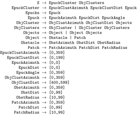
Figure 2: The grammar defining inputs toepuck.
tion between robots, the detection of coded patches on the floor, and static obstacles in the environment.
The controller code has two significant conditional statements: the first tests whether an obstacle is nearby and if so, directs the robot to take an avoiding action; the second tests for the presence of coded ‘food’ patches on the floor and if a patch is detected, attempts to maintain position over the patch. The testing objective is to exercise the four branches from these two conditional statements during a short ‘mission’ lasting the equivalent of 10 seconds in the simulation.
A test input is a configuration of the robot’s environment in which the mission occurs, consisting of fixed circular arena and a number of obstacles and patches.
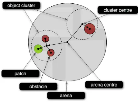
The configuration is described by the grammar listed in figure 2, which defines obstacles and patches in terms of groups we call object clusters. An example of two clusters is shown in figure 3. The objects in the cluster— obstacles and patches—are defined using distances and angles from the centre of the cluster.
The recursion in the grammar permits different numbers of object clusters, each with different numbers of obstacles and patches, to be generated. Parti-tioned variables are used to generate the positions of clusters, obstacles, patches, and e-pucks; and the radii of obstacles and patches.
Strings generated by the grammar are interpreted by a test harness and used to configure the simulated environment. To avoid unrealistic environments, only the first three obstacles and first three patches are configured. The grammar is able to define the initial positions of multiple e-pucks, but in this empirical work only the first e-puck specified by the generated string is added to the arena.
object cluster
arena centre cluster centre
arena patch
[image:15.612.190.417.129.297.2]obstacle
Figure 3: The mission environment specified in terms of object clusters.
mission duration of 10 seconds is equivalent to 500 time steps in the simulation. While the real-world elapsed time for each simulated mission is much less than a second, this is nevertheless much longer than the execution of time of the other SUTs used in this empirical work.
4.2.3. SUT: replace
The C program replace takes three arguments: a target string, a regular expression, and a replacement string. The program subsitutes the replacement string for each substring matching the regular expression in the target string.
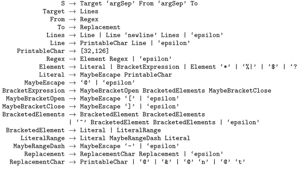
A regular expression is highly structured and so a grammar is a natural choice for representing the input domain of this SUT. The grammar we use for this purpose is shown in figure 4.
The grammar emits a string of terminals that is split by the test harness into the three arguments; the terminal‘argSep’marks the points at which this split occurs. The target string argument is constructed by the rules for variables Lines,Line, andPrintableCharthat emit a string that may include new line control codes (terminal‘newline’). Optional recursion in these rules enable the generation of strings of different lengths and spanning different numbers of lines; the rules producing the terminal epsilon, which is interpreted by the test harness as the empty string, avoid infinite recursion. The variable PrintableCharis the only partitioned variable in the grammar and outputs an integer that is interpreted by the test harness as a single ASCII character; the range 32 to 126 corresponds to the printable ASCII characters.
The regular expression argument is constructed as a sequence of elements by the rules for the variable‘Regex’. The elements may be:
• literals or ranges of literals (optionally negated by the metacharacter‘^’) enclosed in square brackets that match a single occurence of any of the literal characters in the target string (variableBracketExpression); • an element followed by the metacharacter‘*’that matches zero or more
occurrences of the element;
• the metacharacter‘%’that matches the start of the target string; • the metacharacter‘$’that matches the end of the target string;
• the metacharacter‘?’ that matches a single occurrence of any character. (Note that some of the metacharacters used by the replace SUT are non-standard: for example, the POSIX standard uses‘^’to match the start of the string, and‘.’ to match a single occurrence of any character.)
In order to check the parsing and error-handling code in the SUT, it is nec-essary to generate, in addition to well-formed regular expressions, expressions that are ‘nearly’ well-formed such as a bracketed expression missing the closing square bracket. This is achieved by rules associated with variables whose names have the prefixMaybe. As an alternative to returning the correct metacharacter, these variables may omit it, either by preceding it with the escape metacharac-ter, ‘@’, to revert the metacharacter to a standard character, or by returning the empty string,‘epsilon’, instead.
The replacement string argument is constructed by the variableReplacement. It emits a variable-length sequence consisting of printable characters, escape metacharacters, a metacharacter‘&’ that is expanded on replacement by the substring of the target matched by the regular expression, and special character sequences for new line and tab control characters respectively.
In the absence of a functional specification for the SUT, this grammar was constructed using a knowledge of standard regular expressions and a manual re-view of the SUT’s code. For example, the (somewhat non-standard) metachar-acters are defined at the beginning of the code.
This SUT was chosen as a case study since the grammar requires only one partitioned variable, in contrast to the four or more partitioned variables in the grammars used for the preceding two SUTs. We therefore suspect that there may be little, if any, benefit in the use of dynamic partitioning. In addition, both well-formed and malformed structured inputs, as well as inputs that exceed the size of working buffers, are required to fully exercise the program and this requires a relatively complex grammar that we speculate may be hard for the search algorithm to optimise.
S→Target ‘argSep’ From ‘argSep’ To Target →Lines
From →Regex To →Replacement
Lines→Line | Line ‘newline’ Lines | ‘epsilon’ Line →PrintableChar Line | ‘epsilon’ PrintableChar →[32,126]
Regex→Element Regex | ‘epsilon’
Element→Literal | BracketExpression | Element ‘*’ | ‘%|’ | ‘$’ | ‘?’ Literal→MaybeEscape PrintableChar
MaybeEscape →‘@’ | ‘epsilon’
BracketExpression →MaybeBracketOpen BracketedElements MaybeBracketClose MaybeBracketOpen→MaybeEscape ‘[’ | ‘epsilon’
[image:17.612.153.452.125.298.2]MaybeBracketClose →MaybeEscape ‘]’ | ‘epsilon’ BracketedElements →BracketedElement BracketedElements
| ‘^’ BracketedElement BracketedElements | ‘epsilon’ BracketedElement→Literal | LiteralRange
LiteralRange→Literal MaybeRangeDash Literal MaybeRangeDash→MaybeEscape ‘-’ | ‘epsilon’
Replacement →ReplacementChar Replacement | ‘epsilon’ ReplacementChar →PrintableChar | ‘@’ | ‘&’ | ‘@’ ‘n’ | ‘@’ ‘t’
Figure 4: The grammar defining inputs toreplace.
argument errors and read from standard input: these were the code sections that were modified from the original standalone version of the SUT; the remaining instrumented functions constitute 530 lines. In addition, four branches that were identified as unreachable in the code, as well as in notes provided with the source code in the Software-artifact Infrastructure Repository, are also excluded from the set of coverage elements. (As a check on the correctness of this identification, assertions were added at the end point of each of these unreachable branches. None of these assertions failed during the experimentation even though the SUT was exercised many billions of times with a wide variety of randomly generated inputs.)
4.2.4. SUT: tcas
The previous Bayesian network representation could be applied only to SUTs with inputs consisting of a fixed number of ordinal arguments (Poulding and Clark, 2010; Poulding et al., 2011). In order to demonstrate that the new grammar-based representation is also practical for SUTs with this type of input domain, we include a common example from the testing literature: the Traffic Collision Avoidance System (TCAS) used by commercial aircraft. The code is provided by the Software-artifact Infrastructure Repository.
The SUT takes 12 integer arguments, and thus the grammar consists only of 12 partitioned variables—one for each argument—plus the start variable (fig-ure 5). This simple grammar always processes each variable exactly once and always in the same order. For this (and similar) grammars, the fixed generation order enables the search space to be reduced by setting an algorithm param-eter that restricts the conditional dependencies between variables: the parent variable must be processed earlier than child for a dependency to be created, otherwise the dependency would have no effect.
S→ A1 A2 A3 A4 A5 A6 A7 A8 A9 A10 A11 A12 A1→ [0,39999]
A2→ [0,1] A3→ [0,1] A4→ [0,39999] A5→ [0,4999] A6→ [0,39999] A7→ [0,3] A8→ [0,39999] A9→ [0,39999] A10→ [0,2] A11→ [1,2] A12→ [0,1]
Figure 5: The grammar defining inputs totcas.
Boolean predicates) in both conditional and assignment statements.
4.3. Algorithm Implementation
The search algorithm was implemented in C++, and the instrumented SUTs were linked with the algorithm to form a single executable. It would be possible to run the SUTs as separate executables, but the empirical work described below in section 4.4 requires very many algorithm trials and so the overhead of com-munication between the algorithm and SUT running in different processes could increase the time required for the experimentation significantly. The algorithm uses a 64-bit implementation of Marsaglia’s XORShift algorithm (Marsaglia, 2003) to generate pseudo-random numbers. Each trial described in the empiri-cal work used a different seed to the generator; the random seeds were obtained from the QRNG Service (Humboldt-Universit¨at zu Berlin, 2013).
4.4. Empirical Method
To evaluate the two propositions described above, we consider five variants of the algorithm:
1. The full algorithm as described in section 3 (we denote this variantAfull).
2. A variant in which conditional production weights are omitted (we denote this variant A/cond to indicate conditional production weights have been
removed).
3. A variant in which dynamic partitioning of ordinal ranges is omitted; instead a single bin is used for the entire range of the variable (A/part).
We do not explicitly consider a variant in which there is a bin for each single value: for SUTs with large ranges such as tcas, it is clear that such a representation would be infeasibly large. Instead, we consider here the alternative solution proposed in section 3.1.2: that of a fixed uniform distribution over the range of the variable.
4. A variant in which both conditional production weightsanddynamic par-titioning are omitted (A/both).
5. A variant of the full algorithm that uses random search in place of hill climbing (Arand). This is implemented by creating an entirely random
mutation operators. The random neighour is generated in the same way as the initial random profile (see section 3.3.1).
By measuring the difference in performance between the full algorithmAfull,
and the three variants,A/cond, A/part,A/both, that omit one or both of
condi-tional production weights or dynamic partitioning, we may evaluate our hy-pothesis that these features of the grammar-based representation facilitate the search algorithm.
The variantArandevaluates a large number of different, randomly-chosen
in-put profiles. We will interpret the best minumum coverage probability attained by this variant as indicative of the probability achievable by an arbitrarily-chosen profile, and use it as a baseline against which to assess the benefit of using full search algorithm to optimise the profile.
Our measure of performance in comparing the algorithm variants is the computing resource required to derive an input profile satisfying the adequacy criterion of statistical testing, i.e. a profile with a minimum coverage probability equal to or greater than a target value. To aid replicability of the experiments, we measure the computing resource in terms of the total number of times the instrumented SUT is executed for the purpose of evaluating fitness of candidate profiles. Alternative measures of the computing resources consumed, such as the wall-clock or processor time, would be dependent on the algorithm’s imple-mentation and the hardware on which it executes. Since the execution of the instrumented SUT is the most resource-intensive part of the algorithm, the num-ber of SUT executions correlates well with the computing resource consumed, but is independent of both implementation and hardware.
The performance of each algorithm variant is likely to be highly dependent on its parameters—of which there are 10 of consequence for the full algorithm variant—and so we must consider how to set the parameters so as to permit a reliable comparison between the algorithm comparisons. A possible approach is to choose arbitrary parameter settings and use these settings for all five of the algorithm variants. While such an approach would not intentionally introduce a bias in favour of any of the variants, it is nonetheless possible that these arbitrary settings may by chance be near-optimal for one of the variants, but not the others. The comparisons between algorithm variants would be unreliable if such a bias were to occur.
The empirical method therefore consists of two steps: first the parameter settings are tuned for each of the algorithm variants, and then the performance of the algorithm variants are measured at the tuned parameter settings. These steps are described in detail in the following two subsections.
4.5. Parameter Tuning 4.5.1. Approach
A form of response surface methodology is used to tune the algorithm pa-rameters. Response surface methodologies enable the relationship between the response (here, the algorithm’s performance) and the factors on which the re-sponse depends (here, the algorithm’s parameter settings) to be modelled math-ematically; Myers et al. (2004) provide a survey of these techniques. We have previously found the use of such methodologies effective in tuning the param-eters of metaheuristic search algorithms (White and Poulding, 2009; Poulding et al., 2011), and they have a number of advantages over more naive approaches such as tuning one factor at a time while fixing the remaining parameters. Firstly, an appropriate choice of mathematical model can accommodate the de-pendencies between the parameter settings that are likely to exist. Secondly, by choosing efficient experimental designs—i.e. the different parameter settings at which the algorithm is run—an accurate model may be created from the results of relatively few algorithm runs. Thirdly, we can ensure that an equivalent ef-fort is applied to tuning each of the algorithm variant by using the same type of experimental design for each, even though the number of parameters differs between variants.
The methodology we use here has three phases:
• Algorithm trials are performed at a number different parameter settings and the response of the algorithm, i.e. its performance across all four SUTs, recorded.
• A mathematical model is fitted to the results that describes how the re-sponse changes with the parameter settings.
• The parameter settings that optimise the response of the model are de-rived analytically. If there is a reasonable fit between the model and the true response surface, these settings should also be near-optimal for the algorithm.
4.5.2. Parameters
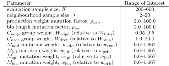
The algorithm parameters to be tuned are listed in table 1. The effect of each of these parameters is described in section 3. Note that the weightsWbins
andwprbtake fixed values, and the other weights are expressed as ratios relative
to these fixed values. The parametersWedge andwadd are not used by variants
A/cond andA/both; the parametersρlen,wjoi,wspl, andwlen are not used by the
variantsA/cond and andA/both.
We do not optimise separately for theArandvariant since it evaluates a
Parameter Range of Interest
evaluation sample size,K 200–600
neighbourhood sample size,λ 2–20
production weight mutation factor,ρprb 2.0–100.0
bin length mutation factor,ρlen 2.0–100.0
Gedgegroup weight,Wedge(relative toWbins) 0.05–0.5
Gdrctgroup weight,Wdrct(relative toWbins) 1.0–20.0
Maddmutation weight,wadd(relative towrem) 0.6–1.667
Mjoimutation weight,wjoi(relative towprb) 0.6–1.667
Msplmutation weight,wspl(relative towjoi) 0.6–1.667
[image:21.612.169.438.124.230.2]Mlenmutation weight,wlen(relative towprb) 0.6–1.667
Table 1: Tunable algorithm parameter settings.
ForArand, we will use the tuned values of the evaluation sample size, K, and
neighbourhood sample size, λ, for the variant Afull in order to enable a fair
comparison between these two variants.
The column ‘Range of Interest’ in the table specifies sensible (although nec-essarily subjective) minimum and maximum settings for each parameter. We make the assumption that the optimal parameter setting lies within this range, and therefore fit the model only over a ‘region of interest’ in the parameter space defined by these ranges.
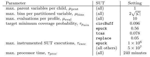
Table 2 lists algorithm parameter settings that are fixed. The parameters µprnt,µbins, andµeval are upper limits on the number of parents per child and
the number of bins in a partitioned variable (see section 3.3), and the number of times a profile may be resampled (section 3.2), respectively. Since these limits are likely to have an effect during relatively few of the algorithm trials and may not be reached in most others, they are difficult model using response surface methodology; for this reason we set them instead to fixed values that were found to be effective for the previous Bayesian network representation in our earlier work (Poulding, 2013).
The parametersτpmin,τexec, andτprocspecify the termination conditions for
the algorithm. τpmin is the SUT-specific target minimum coverage probability,
and is set to approximately 80% of the best value observed in earlier work or during exploratory experimentation: the algorithm terminates if a candidate profile with this fitness or better is found. The algorithm also terminates once τexecexecutions of the instrumented SUT have been performed. This is a
practi-cal consideration: it avoids excessively long-running algorithm trials should the algorithm fail to derive a suitable input profile. The setting of this parameter forepuckis much lower for this SUT than the three others since an execution of epuck takes substantially longer: each execution is a complete run of the simulation.
Parameter SUT Setting
max. parent variables per child,µprnt (all) 1
max. bins per partitioned variable,µbins (all) 2
|C|
max. evaluations per profile,µeval (all) 10
target minimum coverage probability,τpmin circBuff 0.096
epuck 0.56
tcas 0.078
replace 0.05
max. instrumented SUT executions,τexec epuck 1×10⁶
(all others) 5×10⁷
[image:22.612.159.448.123.233.2]max. processor time,τproc (all) 240 minutes
Table 2: Fixed algorithm parameter settings. (|C|is the number of coverage elements.)
the SUT to take multiple seconds or even minutes. (An example of such an input is a regular expression which contains both literals and a long series of the ‘*’ and ‘?’ metacharacters. We suspect the long execution time is because the SUT must evaluate a very large number of possible matches to this regular expression in the target string.) Thus while the algorithm can take as little as a minute to perform 5×10⁷ executions of the SUT, other trials may not
terminate after many hours should they, by chance, generate inputs that cause the execution time of the SUT to be of the order of seconds. For this reason, the parameterτprocspecifies that the algorithm should terminate after 240 minutes
of processor time.
4.5.3. Model
A quadratic linear model is used to describe the relationship between the algorithm’s performance and the parameter settings. This model has the form:
y=β0+
i
βixi+
i
j<i
βi,jxixj+
i
βi,ix2i +ǫ (3)
The independent variables,xi, are the settings taken by the tunable parame-ters to the algorithm variant (iis an index between 1 and the number of tunable parameters). The independent variable,y, is the algorithm’s performance. The coefficients, β, specify how the performance changes with the parameter set-tings, and it is the value of these coefficients that specify the model and must be estimated from the results of performing a number of algorithm trials at selected values of the settings. The random variableǫaccounts for variance (or ‘noise’) in the observed performance that cannot be described by the model. For this algorithm, the only source of noise arises from the stochastic nature of the algorithm: different performances will be observed for repeated trials at the same parameter settings since the algorithm uses a different sequence of pseudo-random numbers for each trial.
as a smooth peak is likely to be simplification; our earlier work on tuning the pa-rameters of the algorithm using the Bayesian network representation suggested a much more rugged surface (Poulding, 2013). As a result of this simplication, the tuned parameters resulting from the methodology used here are unlikely to be the optimal parameter settings. However, the objective of the tuning is only to find ‘near-optimal’ parameter setting specific to each algorithm variant so that a reliable comparison can be made between variants; it is not necessary to find the true optimal parameters. Therefore, we accept the use of the relatively simple quadratic linear model.
For the mutation factor (ρ) and weight (W and w) algorithm parameters, we equate the model parameter,xi, to thelogarithm of the corresponding algo-rithm parameter value. The motivation is that these algoalgo-rithm parameters are ratios—either as a result of their action (the mutation factors) or because they are expressed relative to fixed weight (the group and operator weights)—and we argue as follows that the logarithm is a natural transformation for ratios in a linear model. It is reasonable to expect that a change in such a ratio parameter from 1.0 to 1.1 would have more of an effect on algorithm performance than a change from 10.0 to 10.1. However, in the absence of a logarithm transforma-tion, the model would predict the same change in algorithm performance for both since the model is linear in the parameters. By applying a logarithm trans-formation, the model predicts that a ratio parameter change from 1.0 to 1.1 will now have the same effect as a change of 10 to 11 since, after the transformation, it is the multiplicative rather the additive difference in the algorithm parameter that is modelled.
4.5.4. Experimental Design
A faced central composite design is used to determine the parameter settings (design points) at which to run algorithm trials for the purpose of estimating the model coefficients.
This experimental design specifies design points that are combinations of the ends and midpoints of the range of interest of each algorithm parameter (listed in table 1). A central composite design is effective for determining the model coefficients of a quadratic linear model, but requires fewer algorithm trials than, for example, a full factorial design, for the relatively large number of parameters that the algorithm variants have. A central composite design for the 10 parameters tuned forAfull specifies 178 design points, while a
(two-level) factorial design specifies 1024 design points. Moreover all of the design points of the factorial design are corners of the region of interest, while the faced central composite additionally explores midpoints of faces and the interior of the region. (The NIST/SEMATECH e-Handbook of Statistical Methods provides good overview of the central composite design and the faced variant (National Institute of Standards and Technology, 2013).)
algorithm trials were run in order to tune the settings for algorithm variant Afull. The total number of trials run to tune the variantsA/cond (which has 8
parameters and so a smaller central composite design), A/part (6 parameters),
andA/both (4 parameters) was 6,400; 3,776; and 2,304 respectively.
4.5.5. Response Measure
As discussed above, our chosen measure of algorithm performance is the total number of executions of the instrumeted SUT required by the algorithm to derive an input profile that has the target minimum coverage probability.
However, it is possible that a significant proportion of the algorithm trials may not derive such an input profile before the trial is terminated as result of reaching the limit on the number of executions or on the processer time. Such ‘failed’ trials do not provide a measure of algorithm performance according to the definition above. Nevertheless we can obtain some useful information from such trials: if at parameter settings S, the best profile derived by a trial has a higher minimum coverage probability than the best profile derived by a trial at parameter settings T, then even though neither profile attains the target probability, we may infer that settingsS are better thanT. To incorporate this guidance, we calculate the following response,y for each trial:
ytrial=Nexecs·
τpmin min{pmin, τpmin}
(4)
whereNexecs is the total number of SUT executions performed when the
algo-rithm terminated,τpmin is the target minimum coverage probability, andpminis
the minimum coverage probability of the best profile derived by the trial. If the trial terminated as a result of attaining the target probability, then this equa-tion simply returns the number of execuequa-tions as the response. Otherwise, the response is adjusted to a larger value in the proportion to the degree to the trial missed the target probability. For trials that terminated as a result of exceeding the limit on processor time,Nexecsis set to the value of the parameterτexec, the
limit on the number of executions on the conservative assumption that the trial would have made no further improvement even if it had been permitted further processor time.
At each design point, a summary response is calculated for each SUT as the median value of the values ofytrial, calculated according to equation (4), across
the 16 algorithm trials for that SUT. This summary response will contain less stochastic noise than the individual trials. The summary responses for the four SUTs are then combined using a geometric mean to give a single response for the design point:
ypoint = (ycircBuff·yepuck·ytcas·yreplace)
1
4 (5)
whereycircBuff is the summary reponse for the SUTcircBuff, etc. The use of
overwhelmed by the responses of the other SUTs if they were combined using the arithmetic mean.
Finally the single response at the design point is transformed by taking the logarithm. It was found that by applying this transformation, the variance in the noise term,ǫ, of the fitted model is similar at all magnitudes of the response, and the distribution of the noise is less skewed. Both these characteristics facilitate a more accurate estimation of the model coefficients.
4.5.6. Computing Environment
The algorithm trials were run on a computing grid of 380 CPU cores. The servers forming the grid had a variety of hardware specifications, but resources available for each trial were typical of a desktop PC: a CPU core with a clock speed between 2 and 3 GHz, and a minimum of 1 GB of RAM.
4.5.7. Analysis
Linear regression was used to fit the quadractic linear model from the results obtained from the algorithm trials. The input to this analysis was the exper-imental design and the measured responses calculated as described above; the output was the estimated values of the model coefficients, i.e. theβ coefficients of equation (3).
The optimum parameter settings were predicted from the fitted model using a sequential quadratic programming optimisation algorithm that constrains so-lutions to the region of interest defined by the parameter ranges of table 1. The optimum settings are those that the model estimates will permit the algorithm to find input profiles in the fewest number of executions of the instrumented SUT.
The linear regression and sequential quadratic programming analyses were performed in Matlab, using the functionsregressandfmincon(using the ‘sqp’ algorithm), respectively.
4.5.8. Parameter Tuning Results
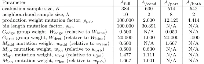
The tuned parameter settings for each of the four variants are listed in table 3. (As discussed above, we do not independently tune the parameter settings of theArand variant: instead, the settings forK and λare taken from
the settings ofAfull, and the other parameters are not applicable.)
The objective of the tuning process was to apply an equivalent effort to finding the best parameter setting for each of the variants, and given the relative simplicity of the quadratic linear model, we do not expect the tuned parameters to necessarily be optimal. Nevertheless it is possible to quantify how well the model fits the observed algorithm performance at each design point using the coefficient of determination (R2) statistic reported by the regression analysis.
Parameter Afull A/cond A/part A/both
evaluation sample size,K 384 600 514 542
neighbourhood sample size,λ 10 2 8 2
production weight mutation factor,ρprb 100.000 2.000 12.125 4.414
bin length mutation factor,ρlen 100.000 30.391 N/A N/A
Gedgegroup weight,Wedge(relative toWbins) 0.500 N/A 0.050 N/A
Gdrctgroup weight,Wdrct(relative toWbins) 20.000 1.000 20.000 1.000
Maddmutation weight,wadd(relative towrem) 0.600 N/A 1.667 N/A
Mjoimutation weight,wjoi(relative towprb) 0.600 0.830 N/A N/A
Msplmutation weight,wspl(relative towjoi) 1.477 1.111 N/A N/A
[image:26.612.139.473.125.230.2]Mlenmutation weight,wlen(relative towprb) 1.667 1.001 N/A N/A
Table 3: The tuned parameter settings for each of the four algorithm variants. ‘N/A’ indicates that the parameter is not applicable to the algorithm variant.
0.948 for the model forAfullwhich we argue is indicative of a good fit given the
stochastic nature of the algorithm, to 0.678 forA/part, which is a poorer fit.
4.6. Algorithm Performance Measurement 4.6.1. Method
In the second step of the empirical method, the performance of each the five tuned algorithm variants is measured for each of the four SUTs. For each combination of algorithm variant and SUT, 64 trials were run, each using a different seed to the pseudo-random number generator. The parameters were set to the tuned values listed in table 3.
As discussed above, our chosen measure of performance is the computing resource required to derive an input profile with a minimum coverage probability equal to or greater than a target value. However, the comparison between algorithm variants could be dependent on the specific target chosen for the probability. To avoid this threat to validity, we do not set a target, but instead run each trial for a fixed number of executions of the instrumented SUT, and after each iteration of the search, record the best minimum coverage probability derived so far and the number of SUT executions made. This data enables us to compare the number of executions required to attain a range of target probabilities. The limit on the number of SUT executions,τexec, was 2×10⁶for
epuck, and 1×10⁸for the other three SUTs: twice the values used in the tuning
trials (table 2). Correspondingly, the processor time limit,τproc, was set at 480
minutes. When analysing the results we make the conservative assumption that for trials terminated by processor time criterion, the minimum coverage probability that would have been attained if the trial had been permitted to run for more SUT executions is the probability that was attained at the point of termination.
4.6.2. Algorithm Performance Results
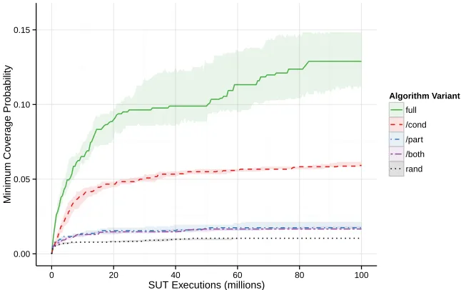
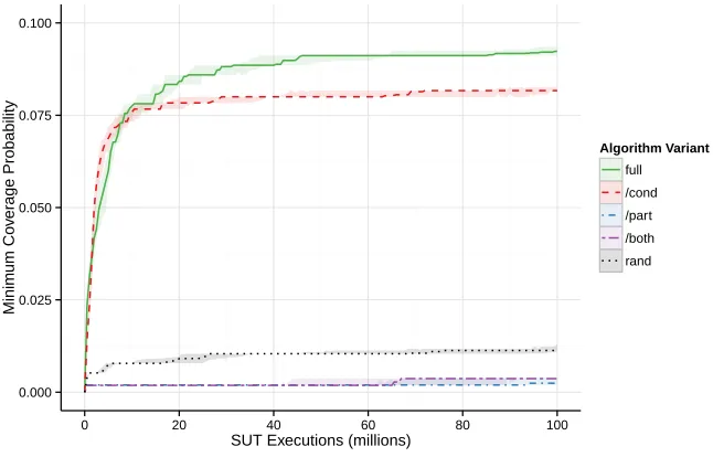
on the x-axis. The shaded ribbons surrounding the lines indicate 95% con-fidence intervals for the median value and these intervals were calculated by bootstrap resampling. We will consider differences in the probabilities of lines for which the ribbons do not overlap as statistically significant. (The raw data from the algorithm trials is available at: http://www.cs.york.ac.uk/~smp/ supplemental/.)
4.7. Discussion
In this discussion, we interpret figures 6–9 as follows. If we were,a priori, to set a limit on the computing resources consumed by the search algorithm (expressed in terms of the number of executions of the instrumented SUT), the graphs indicate the efficacy (expressed in terms of the minimum coverage probability) that we may expect of the best profile found by the search within that limit. These enables us to compare the impact of the algorithm variants across a wide range of limits on computing resource.
4.7.1. Proposition 1
Our first proposition was that the search algorithm is able to derive effec-tive input profiles in comparison to arbitrary profiles chosen at random. This proposition may be assessed by comparing the minimum coverage probability attained by the full algorithm variant (Afull) with that achieved by the random
algorithm (Arand): the latter algorithm returns the best profile from a large
number of profiles chosen at random. For all four SUTs, the profiles derived by Afull have significantly higher minimum coverage probabilities than Arand for
almost all limits on the number of SUT executions.
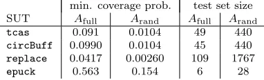
The practical implication of these differences in efficacy may be illustrated by picking a specific limit on SUT executions and calculating the size of the test set generated from the profiles that is necessary to ensure that the value ofQmin—
the minimum probability of any coverage elementbeing exercised by the test set, defined in section 2.1—is suitably close to 1 so that there is a good chance that all the coverage elements are exercised by the test set. We select a limit on SUT executations at the midpoint of the graphs of figures 6–9, i.e. 1×10⁶ for
epuck, and 5×10⁷for the other three SUTs, and assess the minimum coverage
probability attained at the limit. We choose a value for Qmin of 0.99, and
calculate the corresponding test size using equation (1). These test sizes are shown in table 4. For all SUTs, the profile derived by search enables a test set size that ranges from 4 times smaller (epuck) to 16 times smaller (replace) than the best random profile. As discussed in section 4.5.2, the search algorithm with these limits on the number of SUT executions takes approximately 20 minutes for these SUTs (although sometimes longer forreplace) on a single CPU core. Thus substantial savings in test set size are possible at the cost of the relatively small amount of computing resource required to run the search algorithm.
4.7.2. Proposition 2
facil-0.00 0.05 0.10 0.15
0 20 40 60 80 100
SUT Executions (millions)
Minim
um Co
v
er
age Probability
Algorithm Variant
[image:28.612.138.461.135.338.2]full /cond /part /both rand
Figure 6: Median minimum coverage probabilities plotted against the number of executions for
each algorithm variant applied to the SUTcircBuff. (fullis the full proposed algorithm; the
variants/cond,/part, and/both omit, respectively, conditional production weights, dynamic
paritioning, and both these features;randis the random search algorithm.)
0.0 0.2 0.4 0.6 0.8
0 0.5 1.0 1.5 2.0
SUT Executions (millions)
Minim
um Co
v
er
age Probability
Algorithm Variant
full /cond /part /both rand
Figure 7: Median minimum coverage probabilities plotted against the number of executions
for each algorithm variant applied to the SUTepuck. (fullis the full proposed algorithm; the
variants/cond,/part, and/both omit, respectively, conditional production weights, dynamic
[image:28.612.140.461.412.618.2]0.00 0.02 0.04 0.06
0 20 40 60 80 100
SUT Executions (millions)
Minim
um Co
v
er
age Probability
Algorithm Variant
[image:29.612.140.461.133.340.2]full /cond /part /both rand
Figure 8: Median minimum coverage probabilities plotted against the number of executions for
each algorithm variant applied to the SUTreplace. (fullis the full proposed algorithm; the
variants/cond,/part, and/both omit, respectively, conditional production weights, dynamic
paritioning, and both these features;randis the random search algorithm.)
0.000 0.025 0.050 0.075 0.100
0 20 40 60 80 100
SUT Executions (millions)
Minim
um Co
v
er
age Probability
Algorithm Variant
full /cond /part /both rand
Figure 9: Median minimum coverage probabilities plotted against the number of executions
for each algorithm variant applied to the SUTtcas. (full is the full proposed algorithm; the
variants/cond,/part, and/both omit, respectively, conditional production weights, dynamic
[image:29.612.139.462.413.620.2]