This is a repository copy of The Reservation Wage Curve: Evidence from the UK. White Rose Research Online URL for this paper:
http://eprints.whiterose.ac.uk/82775/
Article:
Taylor, K.B. and Brown, S. (2015) The Reservation Wage Curve: Evidence from the UK. Economics Letters, 126. pp. 22-24. ISSN 1873-7374
https://doi.org/10.1016/j.econlet.2014.11.014
eprints@whiterose.ac.uk https://eprints.whiterose.ac.uk/
Reuse
Unless indicated otherwise, fulltext items are protected by copyright with all rights reserved. The copyright exception in section 29 of the Copyright, Designs and Patents Act 1988 allows the making of a single copy solely for the purpose of non-commercial research or private study within the limits of fair dealing. The publisher or other rights-holder may allow further reproduction and re-use of this version - refer to the White Rose Research Online record for this item. Where records identify the publisher as the copyright holder, users can verify any specific terms of use on the publisher’s website.
Takedown
If you consider content in White Rose Research Online to be in breach of UK law, please notify us by
The Reservation Wage Curve: Evidence from the UK
Sarah Brown and Karl Taylor#
Department of Economics University of Sheffield
9 Mappin Street Sheffield
S1 4DT UK
ABSTRACT We investigate the relationship between an individuals’ reservation wage and unemployment in the local area district. Largely unexplored in the literature this adds to the work which has examined the association between employee wages and unemployment – the ‘wage curve’.
JEL classification: J64, J31, R23
Keywords: Reservation Wages, Wage Curve, Unemployment
#
2 1. Introduction and Background
Phillips (1958) explored the relationship between the change in wages and aggregate
unemployment, and found that the rate of change in the nominal wage was inversely related
to aggregate unemployment. More recently, Blanchflower and Oswald (1994) have taken a
micro-econometric approach and argued that it is the wage level which is directly related to
regional unemployment. There is a large body of empirical evidence across a number of
countries suggesting that the relationship between the level of market wages and the local
unemployment rate is negative and relatively stable, which is commonly known as the ‘wage
curve’. The focus of the empirical literature to date has been on individuals in employment.
In contrast, we analyse the relationship between local labour market competition and the
reservation wages of the unemployed, the lowest wage at which an individual is willing to
work. For those out of work, we would expect the threshold-wage to induce individuals back
into employment to be influenced by local labour market conditions.
2. Methodology
Letting denote the individual (=1,..N), the local authority district (LAD) (=1,…,J), time
(=1,…,T), the natural logarithm of the reservation wage can be modelled against a set of
covariates and the natural logarithm of the local unemployment rate, , as follows:
log log (1)
This is the typical ‘wage curve’ specification, see Blanchflower and Oswald (1994), and is
adopted by Blien et al. (2012) who model the German ‘reservation wage curve’. The
estimation is usually based on either panel data, hence incorporating an individual fixed
effect , or on repeated (pooled) cross sections, so . The key parameter of interest
reflects the unemployment elasticity of the reservation wage. With respect to the market wage
3
found to be negative at approximately -0.1 across different time periods and countries
(Blanchflower and Oswald, 2005).
The recent literature has, however, acknowledged shortcomings of the above
specification. In particular, the key covariate of interest – unemployment – is observed at a
higher level of aggregation than the dependent variable. Hence, the parameter estimate will
suffer from aggregation bias. Moreover it may be important to adjust wages for individual
composition effects. Consequently, following Bell et al. (2002) we estimate the reservation
wage curve in two steps. The first stage models reservation wages using a panel fixed effects
estimator to control for unobservable time invariant characteristics :
log (2)
The model also includes LAD dummies, , which can be interpreted as the average
reservation wage in the local labour market, corrected for composition effects. In the second
stage, reservation wage curves are estimated using the composition corrected reservation
wage as the dependent variable:
log log (3)
To account for reservation wage inertia, the model is dynamic and includes LAD and time
fixed effects, denoted by and , respectively. The key covariate of interest is the natural
logarithm of unemployment, denoted by which is also included as a lag to allow for
possible delays in reservation wages responding to competition in the local labour market.
3. Data
We use the British Household Panel Survey (BHPS), a survey conducted by the Institute for
Social and Economic Research comprising approximately 10,000 annual individual
interviews, from 1991 to 2008. In the BHPS, if the respondent ‘is not currently working but
has looked for work or has not looked for work in last four weeks but would like a job’,
4
job?’ Individuals are then asked: ‘About how many hours in a week would you expect to have
to work for that pay?’ From this information we construct hourly reservation wages. We
focus on an unbalanced panel NT=12,147 observations over the period 1992 to 2008 which
consists of 5,721 individuals.1 Around 58% are typically classified as ‘economically
inactive’. We include these individuals in the sample if they report a reservation wage since
they are arguably signalling labour market attachment (see Blackaby et al., 2007). Figure 1
shows the distribution of the natural logarithm of the hourly reservation wage, which is 1.39
(£4.42), on average, over the period.
Following the existing literature, control variables in include: a quadratic term in
the number of years of current labour market state; the natural logarithm of pay in
previous/last job; the natural logarithm of household labour income; the natural logarithm of
benefit income received by the individual; an index of job search intensity based on the
number of different types of search undertaken; aged 16 to 24, 25 to 34, 35 to 44, 45 to 54,
and 55 plus (the omitted category); highest educational qualification distinguishing between
degree, teaching or nursing qualification, Advanced (A) level, General Certificate of
Secondary Education (GCSE), CSE grades 2-5, any other qualification and no educational
attainment (the omitted category); whether currently married or cohabiting; the number of
dependent children in the household; whether currently unemployed rather than
‘economically inactive’; and binary indicators controlling for the occupation in which a job is
sought. In terms of local job market competition, we use log unemployment defined at the
LAD level. There are 278 consistent LADs in the BHPS and we match in gender specific
unemployment rates for each LAD over time from the Labour Force Survey.
5 3. Results
The results are shown in Tables 1 (first stage regression) and 2 (the second stage regression).
Individual unobserved fixed effects are clearly important in Table 1 given their statistical
significance and all of the LAD fixed effects are also statistically significant. The reservation
wage is decreasing in the length of the spell of unemployment, consistent with Brown and
Taylor (2013) and Krueger and Mueller (2014). The reservation wage is increasing in the pay
received in the previous/last job and the level of benefit income received, consistent with
previous findings for the UK, e.g. Jones (1989), although both effects are inelastic. Job search
is negatively associated with the reservation wage which suggests that individuals who are
more informed about the labour market may moderate their wage expectations.
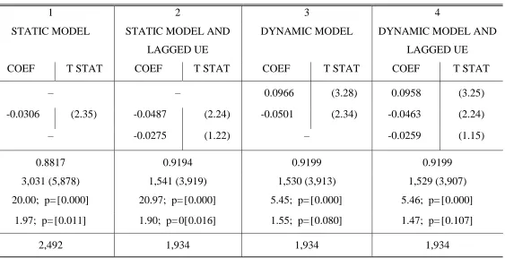
The results of estimating equation (3), the composition adjusted hourly reservation
wage, are shown in Table 2, where four specifications are presented: (1) a static model; (2) a
static model incorporating lagged unemployment thereby allowing for a possible delay in
reservation wages responding to competition in the local labour market; (3) a dynamic model
without lagged unemployment; (4) the full specification of equation (3) incorporating
dynamics and allowing the reservation wage to be influenced by both contemporaneous and
lagged labour market conditions. In each specification, LAD fixed effects are statistically
significant as are time specific effects albeit only in the static specifications. Across each
specification, the effects of unemployment at the LAD level are statistically significant and
negatively associated with the composition adjusted hourly reservation wage with an
elasticity of -0.03 in the static model. Including a lag in local area unemployment suggests
that, contrary to recent estimates of the wage curve for employees, e.g. Longhi (2012),
reservation wage adjustment is contemporaneous.
The final two columns of Table 2 allow for inertia in the reservation wage by
6
the lag composition adjusted reservation wage is positive and statistically significant, as is
commonly found in modelling the wage curve for employees, e.g. Baltagi et al. (2009), but is
relatively small in comparison with a coefficient of approximately 0.1.2 Whether the lag of
unemployment is included has little effect on the elasticity of the reservation wage with
respect to current local area unemployment where the elasticity is around -0.05. This
elasticity is of a similar magnitude to that reported by Blien et al. (2012) for the German
reservation wage curve. The corresponding elasticity for the employee wage curve has
typically been found to be around -0.1, e.g. Blanchflower and Oswald (2005), but more
recent estimates based upon the two-step approach where composition adjusted wages are
constructed have suggested an elasticity of around -0.03 in both Germany and the UK, see
Baltagi et al. (2009) and Longhi (2012), respectively. Hence, our results suggest that the
reservation wage is more sensitive to local labour market conditions in comparison to that of
the market wage curve estimates typically found for employed individuals.
5. Conclusions
In contrast to the existing literature, we have explored how the reservation wage reacts to
local level unemployment rates at a highly disaggregated regional level providing evidence of
the existence of a UK ‘reservation wage curve.’
References
Baltagi, B., Blien, U. and K. Wolf (2009) ‘New evidence on the dynamic wage curve for
Western Germany: 1980–2004.’ Labour Economics, 16, 47-51.
Bell, B., Nickell, S. and G. Quintini (2002) ‘Wage equations, wage curve and all that.’
Labour Economics, 9, 341–360.
Blackaby, D. H., Latreille, P., Murphy, P. D., O’Leary, N. C. and P. J. Sloane (2007) ‘An analysis of reservation wages for the economically inactive.’ Economic Letters, 97, 1-5.
2 In the dynamic model, gives a long-run unemployment elasticity of -0.0555 which is of
7
Blanchflower, D. and A. Oswald (1994) The Wage Curve, MIT Press.
Blanchflower, D. and A. Oswald (2005) The Wage Curve Reloaded. NBER Working Paper,
11338.
Blien, U., Messmann, S. and M. Trappman (2012) ‘Do reservation wages respond to regional unemployment?’ IAB Discussion Paper, 22/2012.
Brown, S. and K. Taylor (2013) ‘Reservation wages, expected wages and unemployment.’
Economics Letters, 119, 276-9.
Jones, S. (1989) ‘Reservation wages and the costs of unemployment.’ Economica, 56, 225-46.
Krueger, A. and A. Mueller (2014) ‘A contribution to the empirics of reservation wages.’ IZA DP. No. 7957.
Longhi, S. (2012) ‘Job competition and the wage curve.’ Regional Studies, 46, 611-20.
Phillips, A.W. (1958) ‘The relation between unemployment and the rate of change of money
wage rates in the United Kingdom, 1861-1957.’ Economica, 25, 283-99.
FIGURE 1: Distribution of the log hourly reservation wage
0
5
10
15
0 1 2 3 4
TABLE 1: First stage estimation results full sample; dependent variable log
COEFFICIENTS T STATISTIC
Intercept 2.5649 (3.75)
Duration of current labour market state -0.0064 (2.01)
Duration of current labour market state squared 0.0002 (1.79)
Log pay previous job 0.0052 (2.40)
Log household labour income 0.0006 (0.30)
Log benefit income 0.0068 (2.23)
Index of job search intensity -0.0101 (2.61)
Whether unemployed -0.0287 (2.05)
Aged 16-24 0.0748 (1.10)
Aged 25-34 0.0989 (1.73)
Aged 35-44 0.0776 (1.66)
Aged 45-54 0.0355 (1.06)
Whether married or cohabiting 0.0237 (1.01)
Number of dependent children -0.0074 (0.82)
Degree 0.1983 (2.56)
Teaching or nursing 0.0752 (1.77)
A level 0.0946 (1.87)
GCSE/ O level 0.0499 (1.05)
CSE 0.0293 (0.39)
Other qualification -0.0211 (0.25)
R squared 0.5248
H0: Individual FE ; F[5720, 3851]; p value 2.19; p= [0.000]
H0: LAD FE ; F[2492, 3851]; p value 1.52; p= [0.000]
OBSERVATIONS (NT) 12,147
TABLE 2: Second stage estimation results full sample; dependent variable composition adjusted reservation wage
1 2 3 4
STATIC MODEL STATIC MODEL AND
LAGGED UE
DYNAMIC MODEL DYNAMIC MODEL AND
LAGGED UE
COEF T STAT COEF T STAT COEF T STAT COEF T STAT
– – 0.0966 (3.28) 0.0958 (3.25)
log -0.0306 (2.35) -0.0487 (2.24) -0.0501 (2.34) -0.0463 (2.24)
log – -0.0275 (1.22) – -0.0259 (1.15)
R squared 0.8817 0.9194 0.9199 0.9199
AIC (BIC) 3,031 (5,878) 1,541 (3,919) 1,530 (3,913) 1,529 (3,907)
H0: ; F statistic; p value 20.00; p= [0.000] 20.97; p= [0.000] 5.45; p= [0.000] 5.46; p= [0.000]
H0: ; F statistic; p value 1.97; p= [0.011] 1.90; p= 0[0.016] 1.55; p= [0.080] 1.47; p= [0.107]
OBSERVATIONS (JT) 2,492 1,934 1,934 1,934