Accelerating Correlated Quantum Chemistry Calculations Using Graphical Processing Units and a Mixed Precision Matrix Multiplication Library

Accelerating Correlated Quantum

Chemistry Calculations Using

Graphical Processing Units and a Mixed

Precision Matrix Multiplication Library

The Harvard community has made this

article openly available.

Please share

how

this access benefits you. Your story matters

Citation Olivares-Amaya, Roberto, Mark A. Watson, Richard G. Edgar, Leslie Vogt, Yihan Shao, and Alán Aspuru-Guzik. 2010. Accelerating

correlated quantum chemistry calculations using graphical

processing units and a mixed-precision matrix multiplication library. Journal of Chemical Theory and Computation 6(1): 135-144.

Published Version doi:10.1021/ct900543q

Citable link http://nrs.harvard.edu/urn-3:HUL.InstRepos:5344469

Accelerating correlated quantum chemistry

calculations using graphical processing units and a

mixed-precision matrix multiplication library

(

MGEMM

₎

Roberto Olivares-Amaya,

Mark A. Watson,

Richard G. Edgar,

Leslie Vogt,

Yihan Shao,

and Alán Aspuru-Guzik

Department of Chemistry and Chemical Biology, Harvard University, Cambridge, Massachusetts

02138., and Q-Chem, Inc. 5001 Baum Blvd, Suite 690, Pittsburgh, PA 15213

E-mail: [email protected]

Abstract

Two new tools for the acceleration of computational chemistry codes using graphical

pro-cessing units (GPUs) are presented. Firstly, we propose a general black-box approach for

the efficient GPU acceleration of matrix-matrix multiplications where the matrix size is too

large for the whole computation to be held in the GPU’s onboard memory. Secondly, we

show how to improve the accuracy of matrix multiplications when using only single-precision

GPU devices by proposing a heterogeneous computing model whereby both single and

dou-ble precision operations are evaluated in a mixed fashion on the GPU and CPU, respectively.

∗_{To whom correspondence should be addressed}

†_{Department of Chemistry and Chemical Biology, Harvard University, Cambridge, Massachusetts 02138.} ‡_{Q-Chem, Inc. 5001 Baum Blvd, Suite 690, Pittsburgh, PA 15213}

The utility of the library is illustrated for quantum chemistry with application to the

acceler-ation of resolution-of-the-identity second-order Møller-Plesset perturbacceler-ation theory (RI-MP2)

calculations for molecules which we were previously unable to treat. In particular, for the

168-atom valinomycin molecule in a cc-pVDZ basis set, we observed speedups of 13.8x, 7.8x

and 10.1x for single-, double- and mixed-precision general matrix multiply (SGEMM,DGEMM

andMGEMM), respectively. The corresponding errors in the correlation energy were reduced

from -10.0 kcal mol−1 to -1.2 kcal mol−1forSGEMMandMGEMM, respectively, while higher

accuracy can be easily achieved with a different choice of cutoff parameter.

1

Introduction

Ever since scientists began to solve the equations of molecular quantum mechanics using numerical

methods and computational tools, the interplay between fundamental theory and application has

been inextricably linked to exponential advances in hardware technology. Indeed, many influential

contributions to quantum chemistry have been motivated by insights into how best to utilize the

available computational resources within the same theoretical model. One example is Almlöf’s

appreciation of the discrepancy that had appeared between data storage capacity and raw processor

speed.1 His subsequent introduction of the Direct SCF technique transformed calculations from

being memory (or disk) bound into being processor bound; previously impossible applications

could be attempted by using additional processor time.

We are now witnessing yet another era in the optimization of quantum chemistry codes,

fol-lowing an explosion of interest in the application of coprocessors such as graphics processing units

(GPUs) to general scientific computing.2This interest in GPUs and related massively-parallel

pro-cessors is largely driven by their tremendous cost to performance ratio (in operation counts per

second per unit of currency) which arises from the economies of scale in their manufacture and

their great demand in numerous multimedia applications. Another key factor in their widespread

uptake for scientific use is the recent release of NVIDIA’s compute unified device architecture

rela-tively simple extension of the standard C language.2

A GPU is an example of a stream-processing architecture3 and can outperform a

general-purpose central processing unit (CPU) for certain tasks because of the intrinsic parallelization

within the device which uses the single instruction, multiple data (SIMD) paradigm. Typical GPUs

contain multiple arithmetic units (streaming processors) which are typically arranged in groups of

eight to form multiprocessors that share fast access memory and an instruction unit; all eight

pro-cessors execute the same instruction thread simultaneously on different data streams. In contrast, in

multiple-core or parallel CPU architectures, each thread must have an instruction explicitly coded

for each piece of data. One of the most recent GPU cards, the Tesla C1060 from NVIDIA, contains

240 streaming processors, can provide up to 933 GFLOPS of single-precision computational

per-formance, and has a cost which is approximately one order of magnitude less than an equivalent

CPU cluster.

GPUs are therefore well-suited to high-performance applications with dense levels of data

par-allelism where very high accuracy is not required. (Although double-precision cards are available,

in the case of NVIDIA GPUs, they have a peak FLOP count approximately 10 times less than

single precision cards.) The challenge for scientists wanting to exploit the efficiency of the GPU

is to expose the SIMD parallelism in their problem and to efficiently implement it on the new

ar-chitecture. A key component of this task is a careful consideration of the memory hierarchy to

efficiently hide memory access latency.

Already, GPUs have been recruited extensively by the scientific community to treat a wide

range of problems, including finite-difference time-domain algorithms,4and n-body problems in

astrophysics.5For computational chemistry, GPUs are emerging as an extremely promising

archi-tecture for molecular dynamics simulations,6,7 quantum Monte Carlo,8 density-functional theory

and self-consistent field calculations9–14and correlated quantum chemistry15methods. Efficiency

gains of between one and three orders of magnitude using NVIDIA graphics cards have been

re-ported compared to conventional implementations on a CPU. In this way, new domains of scientific

supercomputing facilities would have been required.

As an example of the more general impact of accelerator technologies, Brown et. al.16 have

accelerated density-functional theory up to an order of magnitude using a Clearspeed coprocessor.

The Clearspeed hardware is a proprietary compute-oriented stream architecture promising raw

performance comparable to that of modern GPUs, while offering double-precision support and an

extremely low power consumption. The challenges of efficiently utilizing the Clearspeed boards

are similar to those of using GPUs, requiring a fine-grained parallel programming model with

a large number of lightweight threads. Thus, the algorithmic changes suggested for their work

and ours have a common value independently of the precise hardware used, which will of course

change with time.

In the current work, we introduce two new techniques with general utility for the adoption

of GPUs in quantum chemistry. Firstly, we propose a general approach for the efficient GPU

acceleration of matrix-matrix multiplications where the matrix size is too large for the whole

com-putation to be held in the GPU’s onboard memory, requiring the division of the original matrices

into smaller pieces. This is a major issue in quantum chemical calculations where matrix sizes can

be very large.

Secondly, we describe how to improve the accuracy of general matrix-matrix multiplications

when using single-precision GPUs, where the 6-7 significant figures are often insufficient to achieve

‘chemical accuracy’ of 1 kcal/mol. To solve this problem, we have implemented a new algorithm

within a heterogeneous computing model whereby numerically large contributions to the final

result are computed and accumulated on a double-precision device (typically the CPU) and the

remaining small contributions are efficiently treated by the single-precision GPU device.

We have applied these ideas in an extension of our previously published GPU-enabled

im-plementation of resolution-of-the-identity second-order Møller-Plesset perturbation theory

(RI-MP2).17–20 Thus the paper begins in section 2 with an overview of the RI-MP2 method and our

previous GPU implementation. In sections 3 and 4, we discuss our new matrix-multiplication

applying the technology to RI-MP2 calculations on molecules with up to 168 atoms, and we end

the paper with some brief conclusions.

2

GPU acceleration of RI-MP2

One of the most widely-used and computationally least expensive correlated treatments for

elec-tronic structure is second-order Møller-Plesset perturbation theory (MP2). MP2 is known to

pro-duce equilibrium geometries of comparable accuracy to density functional theory (DFT),21 but

unlike many popular DFT functionals is able to capture long-range correlation effects such as the

dispersion interaction. For many weakly bound systems where DFT results are often

question-able, MP2 is essentially the least expensive and most reliable alternative.22 The expression for

computing the MP2 correlation energy takes the form

E(2)=

_∑

(ia|jb)2+1₂[(ia|jb)−(ib|ja)]2

εi+εj−εa−εb

(1)

in terms of the{i,j}occupied and{a,b}virtual molecular orbitals (MOs) that are eigenfunctions

of the Fock operator with eigenvalues{ε}. The MO integrals

(i j|ab) =

_∑

C_µiC_νjC_λaC_σb(µ ν|λ σ) (2)

are obtained by contracting two-electron integrals over the (real) atomic orbital (AO) basis

func-tions

(µ ν|λ σ) = Z Z

φµ(r1)φν(r1)φλ(r2)φσ(r2)dr1dr2 (3)

whereCis the matrix of MO coefficients describing the expansion of each MO as a linear

combi-nation of AOs. One way to considerably reduce the computational cost associated with traditional

the linear-dependence inherent in the product space of atomic orbitals. This allows one to expand

products of AOs as linear combinations of atom-centered auxiliary basis functions,P,

ρµ ν(r) =µ(r)ν(r)≈ρ˜(r) =

∑

and to therefore approximate all costly four-center two-electrons in terms of only two- and

three-center integrals,

g

(µ ν|λ σ) =

_∑

P,Q

(µ ν|P)(P|Q)−1(Q|λ σ) (5)

where we have assumed that the expansion coefficients are determined by minimizing the Coulomb

self-repulsion of the residual density. The result is equivalent to an approximate insertion of the

resolution-of-the-identity (RI).

All our work is implemented in a development version of Q-Chem 3.1,23 where the RI-MP2

correlation energy is evaluated in five steps, as described elsewhere.15 Previously we showed that

step 4, the formation of the approximate MO integrals, was by far the most expensive operation

for medium to large-sized systems, and requires the matrix multiplication

g

(ia|jb)≈

_∑

Bia,QBjb,Q (6)

where

B_ia,Q=

∑

(ia|P) (P|Q)−1/2 (7)

The evaluation of eq 6 is typically an order of magnitude more expensive than eq 7. We shall

concentrate on these two matrix multiplications in this work. Consistent with our previous paper,15

we will repeatedly refer to these evaluations as step 3 (eq 7) and step 4 (eq 6) as we investigate the

accuracy and efficiency of our new GPU implementation.

algebra library, named CUBLAS.24 As previously reported,15 we accelerated the matrix

multipli-cation in eq 6 by simply replacing the BLAS*GEMMroutines with corresponding calls to CUBLAS

SGEMM. This initial effort achieved an overall speedup of 4.3x for the calculation of the

correla-tion energy of the 68-atom doeicosane (C22H46) molecule with a cc-pVDZ basis set using a single

GPU. At this early stage in development, we used the GPU purely as an accelerator for *GEMM

and made no effort to keep data resident on the device.

In the present work, we further explore the acceleration of our RI-MP2 code through the

appli-cation of CUBLAS combined with two new techniques. These enable us to perform more accurate

calculations on larger molecules and basis sets involving larger matrices while also mitigating the

errors associated with single-precision GPUs. We discuss both techniques in the following section.

3

GPU acceleration of GEMM

In large-scale quantum chemistry calculations, the size of the fundamental matrices typically grows

as the square of the number of atomic basis functions (even if the number of non-negligible

ele-ments is much smaller). Moreover, intermediate matrices are sometimes even larger, such as theB

matrices of eq 7.

A GPU can only accelerate a calculation that fits into its onboard memory. While the most

modern cards designed for research can have up to 4 GiB of RAM, consumer level cards may have

as little as 256 MiB (with some portion possibly devoted to the display). If we wish to run large

calculations, but only have a small GPU available, then some means of dividing the calculation up

and staging it through the GPU must be found.

Next, we consider the question of accuracy arising from the use of single-precision GPU cards.

It turns out,13that many operations do not require full double precision support to achieve

accept-able accuracy for chemistry, but, nevertheless, single precision is not always sufficient.

Double-precision (DP) capable GPUs have only become available within the past year, and so are not yet

since the commercial driving force behind such processors is the wealth of multimedia applications

that do not require high precision. We address this problem with the introduction of a new way to

balance the desire for GPU acceleration with a need for high accuracy.

3.1

Cleaving GEMMs

Consider the matrix multiplication

C=A·B (8)

where A is an(m×k) matrix and B is an(k×n)matrix, making C an (m×n) matrix. We can

divideAinto a column vector ofr+1 matrices

A= 

       

A0

A1 .. .

A_r



       

(9)

where each entryAiis a(pi×k)matrix, and∑ri=0pi=m. In practice, all the piwill be the same,

with the possible exception of pr, which will be an edge case. In a similar manner, we can divide

Binto a row vector ofs+1 matrices

B=

B0 B1 · · · Bs

where eachB_j is an(k×q_j)matrix and∑s_j=0qj=n. Again all the qj will be the same, with the

possible exception ofqs. We then form the outer product of these two vectors

C =          A₀ A₁ .. . Ar          ·

B0 B1 · · · Bs (11) =         

A₀·B₀ A₀·B₁ · · · A₀·B_s

A₁·B₀ A₁·B₁ A₁·B_s

..

. . ..

A_r·B₀ A_r·B_s

         (12)

Each individualC_{i j} =A_iB_j is an (p_i×q_j) matrix, and can be computed independently of all the

others. Generalizing this to a full*GEMMimplementation, which includes the possibility of

trans-poses being taken, is tedious but straightforward.

We have implemented this approach for the GPU, as a complete replacement for*GEMM. The

pi and qj values are chosen such that each sub-multiplication fits within the currently available

GPU memory. Each multiplication is staged through the GPU, and the results assembled on the

CPU. This process is hidden from the user code, which simply sees a standard*GEMMcall.

3.2

Heterogeneous computing with MGEMM

With the problem of limited memory solved, we will now demonstrate how to overcome the lack

of double precision GPU hardware. Again, consider the matrix multiplication

We can split each matrix element-wise into ‘large’ and ‘small’ components, giving

C = Alarge+Asmall Blarge+Bsmall

= A·Blarge+Alarge·Bsmall+Asmall·Bsmall

TheAsmallBsmallterm consists entirely of ‘small’ numbers, and can be run in single precision on the

GPU (using the cleaving approach described above, if needed). The other two terms contain ‘large’

numbers, and need to be run in double precision. However, since each of the ‘large’ matrices should

be sparse, these terms each consist of a dense-sparse multiplication. We only store the non-zero

terms of theAlargeandBlargematrices, cutting the computational complexity significantly. Consider

C0_ik=A_{i j}Blarge_jk (14)

Only a fewBlarge_jk will be non-zero, and we consider each in turn. For a particularscalar Blarge_jk,

only the kth column ofC0 will be non-zero, and equal to the product ofBlarge_jk and thecolumn

vector Ai j (where j is fixed by the particularBlargejk we are considering). This non-zero column

vectorC0_ik can be added to the final result,C, and the nextBlarge_jk considered. A similar process

can be applied to theAlargeBsmall term (producingrowvectors ofC). Again, this approach can be

generalized to a full*GEMMimplementation including transposes.

The remaining question is that of splitting the matrices. We have taken the simple approach of

defining a cutoff value,δ. If|Ai j|>δ, that element is considered ‘large,’ otherwise it is considered

to be ‘small.’

We have implemented our algorithm we have dubbed MGEMM, for ‘mixed-precision general

matrix multiply.’ It operates similarly to the other*GEMMroutines, but takes one extra argument

4

MGEMM benchmarks

We will now discuss some benchmarks for MGEMM. Our aim is to assess the speed and accuracy

ofMGEMMfor various matrix structures and choice of cutoff tolerance compared to aDGEMMcall

on the CPU. In particular, it is important to benchmark how much computational speed is gained

using the mixed-precisionMGEMMwith the GPU as a function of the loss in accuracy compared to

DGEMM. Throughout this section, CPU calculations were made using an Intel Xeon E5472

(Harper-town) processor clocked at 3.0 GHz attached to an NVIDIA Tesla C1060 (packaged into a Tesla

S1070). The GPU calls were limited to 256 MiB of RAM to model a more restricted GPU in a

typical BOINC (Berkeley Open Infrastructure for Network Computing) client.25,26

4.1

Using model matrices

0 2 4 6 8 10 12 14 16 18

0 2000 4000 6000 8000 10000 12000

Speed-up relative to CPU DGEMM

Matrix size MGEMM fSalt = 10-2

MGEMM fSalt = 10-3 MGEMM fSalt = 10-4 SGEMM (Cleaver) DGEMM (Cleaver)

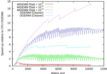
Figure 1: Speedup for various*GEMMcalls as a function of (square) matrix size (averaged over ten

runs). Most elements were in the range[−1,1], with the ‘salt’ values in the range[90,110]. Times are scaled relative to runningDGEMMon the CPU.

In Figure 1 we show the speedup for a variety of *GEMM calls using matrices of increasing

(square) size. Three different types of matrix were considered, based on the number of randomly

scattered ‘large’ elements. All the matrices were initialized with random values in the range[−1,1]

forming the ‘background’, and ‘salted’ with a fraction f_salt of random larger values in the range

[90,110]. The size of theMGEMMcutoff parameterδ was chosen such that all the salted elements

There are threeMGEMMcurves plotted, for different values of f_salt=10−2, 10−3and 10−4. The

SGEMM(cleaver)curve corresponds to doing the full matrix multiplication on the GPU using

the GEMMcleaver and includes the time taken to down-convert the matrices to single precision on

the CPU. TheDGEMM(cleaver)curve corresponds to a full double-precision matrix

multiplica-tion on the GPU, which is possible for modern cards, and we include it for completeness. Square

matrices were used in all cases, with no transpositions in the*GEMMcalls. All the runs were

per-formed ten times and speedups are obtained relative to the time taken for the correspondingDGEMM

call on the CPU.

Examining the results, we see thatSGEMMon the GPU gives a speedup of 17.1x over running

DGEMM on the CPU for a matrix of size 10048×10048, and is even faster for larger matrices.

This represents an upper bound for the speedups we can hope to obtain with MGEMM for such

matrices. The speedups increase significantly as the matrices become larger due to the masking

of memory access latencies and other overheads when employing the GPU for more

compute-intensive processes.

Considering theMGEMMresults, we see that the speedups are strongly dependent on the number

of large elements which must be evaluated in double-precision on the CPU. For the relatively high

value of f_salt=10−2, runningMGEMMwas actually slower than runningDGEMMon the CPU alone.

This is understandable when one considers the extra steps in the MGEMMalgorithm. In addition

to down-converting the matrices to single precision, the CPU has to perform cache-incoherent

operations on the ‘large’ multiplications. We store our matrices column-major, so the operations

performed in eq 14 are cache-coherent. However, it is easy to see that the corresponding operations

forC0=AlargeBsmallwill be cache-incoherent for bothC0andBsmall(recall thatAlargewill be stored

as individual elements). This brings a huge penalty over a standard*GEMMimplementation which

is tiled for cache-coherency.

In contrast, for fsalt=10−4, there is much less penalty to runningMGEMMoverSGEMMon the

GPU, due to the small fraction of large elements computed on the CPU. Speedups of approximately

and speedups of approximately 2x relative to CPUDGEMMare obtained for the largest matrices. In

this caseMGEMMruns approximately 2.5 times slower than fullDGEMMon the GPU (available in

the most modern cards). We may also note that the thresholds for matrix cleaving can be discerned.

They start at matrix sizes of 3344 for double precision and 4729 for single precision. These are

detectable on the curves, but do not alter the times significantly.

1e-05 0.0001 0.001 0.01 0.1 1

0 2000 4000 6000 8000 10000 12000

Maximum error relative to CPU DGEMM

Matrix size

MGEMM fSalt = 10-2 salt = 102 MGEMM fSalt = 10-3 salt = 102 MGEMM fSalt = 10-4 salt = 102 MGEMM fSalt = 10-2 salt = 104 MGEMM fSalt = 10-3 salt = 104 MGEMM fSalt = 10-4 salt = 104 SGEMM fSalt = 10-2 _{salt = 10}2

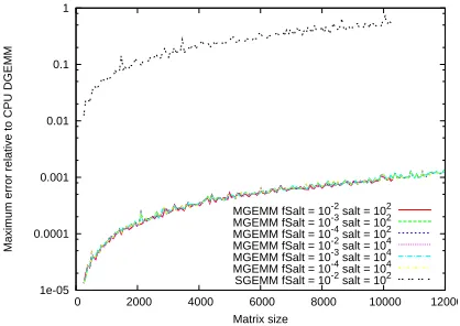
Figure 2: Maximum Absolute Error in a single element for variousGEMM calls as a function of matrix (square) size. Most elements were in the range [−1,1], with the ‘salt’ values in the range [90,110]or[9990,10010]. A CPUDGEMMcall was taken as the reference calculation.

In Figure 2, we examine the accuracy of MGEMM for various matrix structures. Shown in the

figure are the maximum absolute errors of a single element (relative to the CPU DGEMM result)

plotted as a function of matrix size, for different fractions f_salt and sizes of salted values. As

before, all the matrices were initialized with random values in the range[−1,1], but now the salting

sizes were grouped into two ranges: [90,110]and[9990,10010]. There is one curve usingSGEMM

corresponding to a fraction of salted values, f_salt=1%, in the range[90,110], and severalMGEMM

curves.

Looking at the figure, we see that the salted SGEMM calculation produces substantial errors

for the largest matrices, which are of the same order of magnitude as the background elements

themselves. In contrast, the errors are significantly reduced when using MGEMMand are the same

regardless of the fraction or size of the salted elements. In fact, these limitingMGEMMerrors are the

same as the errors observed when usingSGEMMon a pair ofunsaltedrandom matrices. Essentially,

in single precision since the cutoff tolerance guarantees that all the salted contributions will be

computed in double precision on the CPU.

The order of magnitude of the limiting error can be rationalized from a consideration of the

number of single-precision contributions per output element (approximately 1000-10000 in this

case) and the expected error in each (approximately 10−6−10−7for input matrices with a random

background on [−1,1]). A consequence of this observation is that an upper bound to the

maxi-mum error can be estimated from a consideration of only the matrix size and the cutoff parameter

δ, although this estimate will be very conservative in cases where there is no obvious ‘constant

background’, as we shall see in the following.

4.2

Using RI-MP2 matrices

1e-07 1e-06 1e-05 0.0001 0.001 0.01 0.1 1

1e-10 1e-08 1e-06 0.0001 0.01 1 100

Fraction of large elements

Double precision cutoff (ia|P)

(P|Q)1/2 B_ia,Q

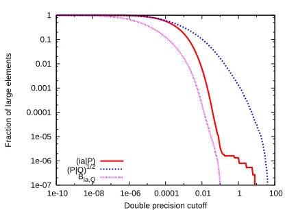
Figure 3: Fraction of ‘large’ elements as a function of the cutoff parameter,δ, for the taxol RI-MP2

matrices in steps 3 and 4 of the algorithm outlined in Sec. 2.

For a more realistic assessment of MGEMM for quantum chemistry applications, we also ran

benchmarks on two pairs of matrices taken from an RI-MP2 calculation on the taxol molecule in a

cc-pVDZ basis, as described below in Section 5. In this case, theMGEMMcutoff parameterδ will

nolonger be dimensionless, but rather will take the same units as the the input matrix elements,

which, for eqs 6 and 7, are all computed in atomic units. For simplicity, we have dropped these

units in the following discussion and assumed their implicit understanding based on the matrices

As summarized in Section 2, our RI-MP2 implementation has two steps involving significant

matrix multiplications. That is, the evaluation of equations 6 and 7. As described in Sec 2 and

consistent with our previous work,15 we shall refer to these two matrix multiplications as step 3

(eq 7) and step 4 (eq 6) throughout the following discussion. Although step 3 is typically an order

of magnitude faster than step 4, we need to take care to study it since we are interested not only in

speed, but also error accumulation usingMGEMM.

For the case of taxol in a cc-pVDZ basis, the full (P|Q)−1/2 matrix is of size 4186×4186.

However, in the Q-Chem implementation, the full (ia|P) and B_ia,Q matrices do not need to be

explicitly constructed. Instead, it is sufficient to loop over discrete batches of i, depending on

available memory. As seen above, larger matrices deliver a greater speedup when multiplied on

the GPU, thus there is a motivation for choosing as large a batch size (overi) as possible in our GPU

calculations. In these test benchmarks, we chose batch sizes of 1 and 7 based on the available CPU

memory such that the(ia|P)andB_ia,Qmatrices have dimensions of 897×4186 and 6279×4186,

respectively. We do not batch the step 3 matrices since there are onlyO(N)multiplications taking

place and the more computationally intensive process is step 4, which has orderO(N2)operations.

We note that the structure of these matrices was found to be very different from the model

matrices considered in the previous subsection. Specifically, the distribution of large and small

elements was structured, as described below. In the case of the(P|Q)−1/2 matrix, involving only

the auxiliary basis set, the large elements were heavily concentrated on the top left-hand corner

in a diagonal fashion, while the other matrices were observed to have a striped vertical pattern of

large elements. In the current implementation, the main issue affecting the efficiency ofMGEMM

is the ratio of large to small elements in the input matrices, but in general we can also expect the

sparsity structure to impact performance. In cases where the structure is known in advance, a more

specialized treatment could give worthwhile speedups, but this is beyond the scope of the current

work.

The precise fractions of large and small elements for the taxol case are plotted in Figure 3 with

curves are only for one particulari-batch, as explained above, and not the full matrices. However,

to ensure that the results are representative of the full matrix, we have checked the distributions

from the other batches, and we chose the most conservative matrices for our plots, which had large

elements across the broadest range ofδ-values.

Looking at the curves, it is significant that the step 3 matrices have a greater fraction of large

elements than the step 4 matrices, and specifically, the (P|Q)−1/2 matrix has the largest elements

of all. This means that for a constantδ-value, we can expectMGEMMto introduce larger errors in

the step 3 matrix multiplications than in step 4. In future work, it could be advantageous to tailor

the δ-value for different steps in an algorithm, or even different input matrices, but in this first

study, we use a constantδ-value throughout any given calculation.

In the model matrices of the previous subsection, the distribution would have resembled a

step function around δ =1.0, rapidly dropping from 1.0 to the chosen fraction of salted values

for δ >1.0, and rapidly stepping again to 0 for δ-values beyond the salt size. In contrast, we

see a continuous decay of element values in the real matrices across many orders of magnitude.

In Figure 1, MGEMM was seen to outperform DGEMMfor a fraction of salts of order 10−4.

Com-paring to Figure 3, this suggests that δ should be greater than 0.01 to ensure significant MGEMM

speedups when considering the (ia|P)andB_ia,Q matrices, while the fraction of large elements in

the(P|Q)−1/2matrices only becomes this small forδ-values of order 10.

Having analyzed the distributions, we can consider their effect on the accuracy and speedups

compared to the model benchmarks. On the top plots of Figure 4 and Figure 5, we show how the

speedup for various*GEMMcalls (compared to a CPUDGEMMcall) varies withδ, averaged over

ten calls. We see that the MGEMM performance varies continuously from being almost the same

speed as CPUDGEMM to reaching the GPU SGEMMlimit for sufficiently large cutoff values. As

expected, for the step 4 matrices, significant speedups are only observed forδ-values greater than

approximately 0.01. Similarly, for step 3, the greatest speedups are only observed for much larger

δ-values, approximately 1 to 2 orders of magnitude greater than for step 4. The limiting values

0 1 2 3 4 5 6

0 0.5 1 1.5 2 2.5 3

Speedup relative to

CPU DGEMM MGEMM Speedup 0 5 10 15 20 25

0 0.5 1 1.5 2 2.5 3

Maximum absolute error

(x10

-7 Hartree

1/2

)

Double precision cut-off MGEMM MAE

SGEMM MAE

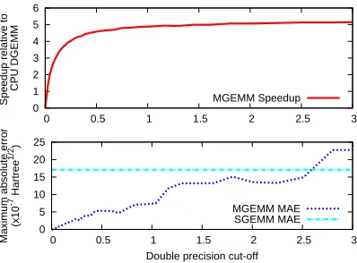
Figure 4: Results from the step 3 matrix multiplication in a taxol RI-MP2 calculation as a function of the cutoff variable δ. Top: MGEMM speedups relative to a CPU DGEMMcalculation. Bottom:

Maximum absolute error (Hartree1/2) in a single element of the output matrix for MGEMM and

SGEMMruns. 0 1 2 3 4 5 6 7 8 9 10

0 0.02 0.04 0.06 0.08 0.1 0.12 0.14

Speedup relative to

CPU DGEMM MGEMM speedup 0 2 4 6 8 10 12 14 16 18

0 0.02 0.04 0.06 0.08 0.1 0.12 0.14

Maximum absolute error

(x10

-9 Hartree)

Double precision cutoff MGEMM MAE

SGEMM MAE

Figure 5: Results from the step 4 matrix multiplication in a taxol RI-MP2 calculation as a function of the cutoff variable δ. Top: MGEMM speedups relative to a CPU DGEMMcalculation. Bottom: Maximum absolute error (Hartree) in a single element of the output matrix forMGEMMandSGEMM

is mainly due to the different sizes of the matrices used in each benchmark, recognizing that the

smaller matrices used in step 3 will give smaller speedups (c.f. Figure 1).

Considering theMGEMMaccuracy, the bottom plots in Figure 4 and Figure 5 show the maximum

absolute errors of a single element (relative to the CPUDGEMMresult) plotted as a function ofδ.

As δ increases, the MGEMM errors steadily increase as expected, with the single precision limit

being approached for sufficiently largeδ. Again we see significant differences between step 3 and

step 4, as expected from the element distributions. Firstly, the errors in step 3 are approximately 2

orders of magnitude greater than in step 4. Moreover, in step 4, the errors reach theSGEMMlimit

forδ ∼0.1, while the errors in step 3 continue to increase for cutoff values an order of magnitude

larger. Examining Figure 3, it is expected that the relatively large fraction of elements greater than

1.0 in the(P|Q)−1/2matrix are responsible for these observations.

Unexpectedly, however, the errors are not seen to steadily converge to theSGEMMlimit for step

3 in the same way as for step 4, with errors largerthanSGEMM being observed forδ >2.5. We

have performed additional tests to understand why this may be happening and our conclusion is

that it results from error cancellation effects. To verify this idea, we repeated similar calculations

replacing all matrix elements with their absolute values, so that any error cancellation would be

essentially removed. The result was a monotonic curve much more similar to that observed for

step 4, showing the same steady convergence to theSGEMMlimit (not shown).

We may now consider the advantages of using MGEMMoverSGEMMin terms of accuracy and

speed. Comparing the subplots in Figure 4 and Figure 5 we can see that for a rather modest

performance decrease from approximately 5x to 4x, and 9x to 7x, for steps 3 and 4 respectively,

an order of magnitude reduction in the errors can be obtained. However, it might be noted that

in all cases the maximum errors are rather small in these tests, being only of order 10−6 in the

worst case. Considering real RI-MP2 applications, we might therefore expect the final errors in

the molecular energy to be almost negligible using single precision only. However, in Sec. 5, the

benchmarks show that for larger molecules the errors propagate such that the resulting correlation

Finally, from Figure 2, we can estimate an upper bound on the maximum absolute error of

each element for differentδ-values. Since the matrix dimension is approximately 4000, the choice

δ=0.1 would give a conservative error bound of approximately 4000∗10−6∗0.1 which is of order

10−4. However, because the matrices do not have a ‘constant background’ of 0.1 this estimate is

very conservative, and the observed error in Figure 5 is much less.

5

RI-MP2 acceleration benchmarks

In this section, our intention is to perform full RI-MP2 quantum chemistry calculations on real

molecules and to benchmark the speedups and accuracy in the resulting molecular energy that

can be obtained when using the GPU. In this case, we include in the timings all steps required to

compute the RI-MP2 correlation energy (after the SCF cycle has finished) while the GPU*GEMM

libraries are used to accelerate the matrix multiplications in steps 3 (eq 7) and 4 (eq 6), as described

in the previous sections. As a result, the observed speedups will be reduced compared to the

previous benchmarks since not all steps are accelerated.

For all these benchmarks, we used an AMD Athlon 5600+ CPU clocked at 2.8 GHz, combined

with an NVIDIA Tesla C1060 GPU with 4 GiB of RAM. For some calculations, the GPU was

limited to 256 MiB of RAM, as described below.

We emphasize that only the latest GPU cards have double-precision support to enable CUBLAS

DGEMM, while older cards also have limited memory which significantly constrains the size of even

the CUBLASSGEMMmatrix multiplications. Our previous attempts to use GPUs to accelerate

RI-MP2 calculations were limited to molecular systems with less than 500 basis functions15 due to

this constraint. However, using the matrix cleaver in the (MGEMM) library, we are now able to run

calculations of a size limited only by the CPU specification, independent of the GPU memory.

For our test systems we chose a set of linear alkanes (C8H18, C16H34, C24H50, C32H66, C40H82)

as well as two molecules of pharmaceutical interest, taxol (C47H51NO14) and valinomycin (C54H90N6O18),

The matrix cleaver andMGEMMwere implemented in a modified version of the Q-Chem 3.1

RI-MP2 code previously described.15Concerning the batching over occupied orbitals, as discussed in

section 4.2, only the step 4 matrices were batched. For taxol, the batch size was 7, as before. For

all molecules, the batch size was chosen dynamically based on the matrix sizes and available CPU

memory (for taxol, this results in a batch size of 7, as used before). However, in these benchmarks

the batching issue is less important since we were limited to only 256 MiB of GPU RAM, which

means that large batches would have to be cleaved by theMGEMMlibrary in any case.

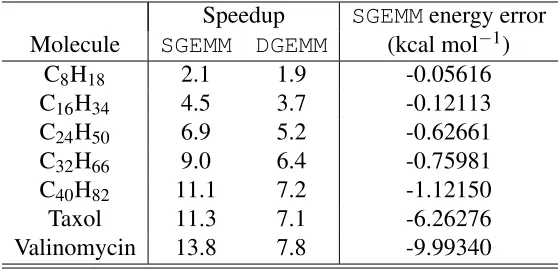
Table 1: Speedups using CUBLAS SGEMM and DGEMM and total energy errors relative to CPU

DGEMMfor various molecules in a cc-pVDZ basis.

Speedup SGEMMenergy error Molecule SGEMM DGEMM (kcal mol−1)

C8H18 2.1 1.9 -0.05616 C16H34 4.5 3.7 -0.12113 C24H50 6.9 5.2 -0.62661 C32H66 9.0 6.4 -0.75981 C40H82 11.1 7.2 -1.12150 Taxol 11.3 7.1 -6.26276 Valinomycin 13.8 7.8 -9.99340

Firstly, in Table 1 we benchmarked the reference case of using either CUBLAS SGEMM or

DGEMMfor each test molecule using the double-ζ basis set. The table shows the speedup in

com-puting the RI-MP2 correlation energy and the error relative to a standard CPU calculation (for

SGEMMonly). The speedups andSGEMMerrors are seen to be greater for the larger molecules, as

expected, with the largest speedups observed for valinomycin at 13.8x and 7.8x, usingSGEMMand

DGEMM, respectively. However, while CUBLASDGEMMgives essentially no loss of accuracy, the

SGEMMerror is approximately -10.0 kcal mol−1, which is well beyond what is generally accepted

as chemical accuracy.

The results from Table 1 highlight the need for MGEMM to reduce the errors when

double-precision GPUs are unavailable. As an initial test ofMGEMMfor this purpose, we repeated the

cal-culation of the taxol molecule in the double-ζ basis set (1123 basis functions) for various choices

0 2 4 6 8 10 12

0 0.5 1 1.5 2 2.5 3 0 0.5 1 1.5 2

Speedup relative to CPU DGEMM

Absolute energy error

Double Precision cut-off MGEMM speedup MGEMM error (kcal mol-1)

Figure 6: TaxolMGEMMcalculation using a double-ζ basis set with respect to the double precision

cutoff (δ). We plot the MGEMM speedup relative to CPU DGEMM and it shows a rapid increase

withδ towards an asymptotic value of 10.6x. We also show the energy difference relative to CPU DGEMM, which is seen to increase steadily over the range ofδ-values chosen, but is significantly

less than the previously computedSGEMMerror of 6.6276 kcal mol−1 .

in the energy.

As the cutoff increases, theMGEMMspeedup increases rapidly to the asymptotic limit of 10.6x,

which is slightly less than theSGEMMlimit of 11.3x due to theMGEMMoverhead. In contrast, the

energy error in this range increases almost linearly towards theSGEMMlimit. Recalling Figure 4

and Figure 5, it seems that the errors are dominated by the step 3 operations, where we form the

B_ia,Q matrices, since these errors are also seen to steadily increase over the range of cutoff values

considered in Figure 6. The overall speedups are also seen to have a similar shape to the step 3

speedups, but are approximately twice as large. This reflects the greater speedups in step 4, noting

that step 4 on the CPU is the most expensive step in the algorithm.

To achieve a target accuracy of 1.0 kcal mol−1, Figure 6 shows that a cutoff value ofδ <2.0

in the case of taxol in a double-ζ basis is necessary. However, trading the accuracy and speedup, a

good choice of cutoff would beδ =1.0. This gives an error of 0.5 kcal mol−1, which is an order

of magnitude smaller than usingSGEMM, with a speedup very close to theMGEMMlimit and only

about 7% less than theSGEMMlimit.

In Table 2, we explore the performance ofMGEMMusing a constant cutoff value ofδ=1.0. The

basis sets. In this particular case, we have limited the GPU to use only 256 MiB of RAM to mimic

the capability of older cards and emphasize the use of theMGEMMcleaver. This will naturally result

in a loss of speedup compared to utilizing a larger GPU memory. In the case of taxol the reduction

is approximately 20%, but obviously still much faster than a calculation using only the CPU.

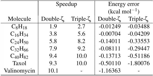
Table 2: MGEMM speedups and total energy errors with respect to CPU DGEMM for various molecules in a cc-pVDZ and cc-pVTZ basis.

Speedup Energy error (kcal mol−1) Molecule Double-ζ Triple-ζ Double-ζ Triple-ζ

C8H18 1.9 2.7 -0.01249 -0.03488 C16H34 3.8 5.6 -0.00704 -0.04209 C24H50 5.8 8.2 -0.14011 -0.33553 C32H66 7.9 9.2 -0.08111 -0.29447 C40H82 9.4 10.0 -0.13713 -0.51186 Taxol 9.3 10.0 -0.50110 -1.80076 Valinomycin 10.1 - -1.16363

-Looking at Table 2, the trends are the same as in Table 1, but the MGEMMerrors are seen to

be approximately an order of magnitude less than the SGEMM errors (for the larger molecules).

For valinomycin in the cc-pVDZ basis, theSGEMMspeedup is reduced from 13.8x to 10.1x using

MGEMM, but the error in the total energy is also reduced from -10.0 kcal mol−1to -1.2 kcal mol−1,

which is now very close to chemical accuracy. Moreover, while CUBLASDGEMMclearly has the

advantage (when available) of not introducing errors, if -1.2 kcal mol−1is an acceptable accuracy,

MGEMMmay even be favoured since theDGEMMspeedup is only 7.8x compared to 10.1x. Moreover,

since the error increases as δ is increased, there will be a substantial error cancellation when

obtaining energy differences. Thus, the apparent error in MGEMM will approach the DGEMM

value.

It is unsurprising that the errors are larger when using the triple-ζ basis. The manner in which

the errors grow can be anticipated using the arguments mentioned in section 4, where we

esti-mate an upper bound on the maximum absolute error fromMGEMMby consideration of a constant

practice, this upper bound can be rather conservative. Moreover, if the quantity of interest is the

final energy, we must also take into account how the matrices are used after the application of

MGEMM(e.g if they are multiplied by large numbers). Nevertheless, a topic of future study could

be the search for a more sophisticated method for determining a safe and optimal δ-value for a

given size of acceptable error in the final energy.

6

Conclusion

We have developed and implemented two new tools for the acceleration of computational

chem-istry codes using graphical processing units (GPUs). Firstly, we proposed a general black-box

approach for the efficient GPU acceleration of matrix-matrix multiplications where the matrix

size is too large for the whole computation to be held in the GPU’s onboard memory. Secondly,

we have shown how to improve the accuracy of matrix multiplications when using only

single-precision GPU devices by proposing a heterogeneous computing model whereby both single and

double precision operations are evaluated in a mixed fashion on the GPU and CPU, respectively.

This matrix cleaver and mixed-precision matrix multiplication algorithm have been combined

into a general library namedMGEMM28 , which may be called like a standardSGEMMfunction call

with only one extra argument, the cutoff parameterδ, which describes the partitioning of single

and double-precision work. Benchmarks of general interest have been performed to document the

library’s performance in terms of accuracy and speed.

Compared to a CPU DGEMMimplementation,MGEMMis shown to give speedups approaching

the CUBLASSGEMMcase when very few operations require double precision, corresponding to a

largeδvalue (which is equivalent to having a large fraction of small elements in the input matrices).

However, when the fraction of large elements approaches 0.1% or greater, much less benefit is

seen. Concerning accuracy,MGEMMrestricts the maximum error in an element of the output matrix

to an upper bound based on the size of the matrix and the choice of δ-value. In practice, this

strongly dependent on the distribution of large and small values in the input matrices, as we have

shown.

To illustrate the utility of MGEMM for quantum chemistry, we have implemented it into the

Q-Chem program package to accelerate RI-MP2 calculations. We have considered both the use

of modern high-end GPU cards, with up to 4 GiB of memory and double-precision capability, as

well as legacy cards with only single-precision capability and potentially only 256 MiB of RAM.

Greater speedups, but also larger absolute errors in the correlation energy were observed with the

larger test molecules. In particular, for the 168-atom valinomycin molecule in a cc-pVDZ basis

set, we observed speedups of 13.8x, 10.1x and 7.8x, forSGEMM,MGEMMandDGEMM, respectively.

The corresponding errors in the correlation energy were -10.0 kcal mol−1, -1.2 kcal mol−1, and

essentially zero, respectively. TheMGEMMδ-value was chosen as 1.0 for these benchmarks.

We have also suggested ways in which the size of the MGEMMerror may be parameterized in

terms of a conservative error bound. In addition, we have observed that the correlation energy error

grows approximately linearly with the choice ofδ-value, which may suggest a route to thea priori

determination of theδ for a given target accuracy.

As we submit this paper for publication, we have become aware of the planned release of the

next-generation GPU from NVIDIA, currently code-named Fermi. This card will have

double-precision support with a peak performance only a factor of 2 less than single-double-precision operations.

However, despite the emergence of double-precision GPU devices, it is our hope that the current

work will provide a framework for thinking about other mixed-precision algorithms. Even with

the more widespread availability of double-precision cards in the future, we have seen howMGEMM

can run faster than CUBLASDGEMMif a specified level of accuracy is tolerated. Indeed, practical

calculations on GPUs are very often bound by memory bandwidth to/from the device, rather than

raw operation count. In these cases, the transfer and processing of only single-precision data could

effectively double the performance compared to naive double-precision calculations.

Moreover, we are interested in the use of commodity GPUs as part of a grid-computing

gaming devices, but most of the client machines will not host the latest high-end hardware. We

therefore see a significant application forMGEMMin leveraging these large numbers of legacy cards

to overcome their lack of RAM and double-precision arithmetic. We are therefore optimistic

over-all about the roleMGEMMcan play in helping to accelerate computations using GPUs in the near

future.

7

Acknowledgments

The authors acknowledge financial support from NSF “Cyber-Enabled Discoveries and

Innova-tions” (CDI) Initiative Award PHY-0835713, as well as NVIDIA. The authors acknowledge

tech-nical support by the High Performance Techtech-nical Computing Center at the Faculty of Arts and

Sciences of Harvard University and the National Nanotechnology Infrastructure Network

Compu-tation project for invaluable support. R.O.A. wishes to thank CONACyT and Fundación Harvard

en México for financial support. L.A.V. acknowledges the NSF for funding. The authors thank

References

(1) Almlöf, J.; Taylor, P. R. InAdvanced Theories and Computational Approaches to the

Elec-tronic Structure of Molecules; Dykstra, C., Ed.; D. Reidel: Dordrecht, 1984; p 107.

(2) CUDA Programming Guide, http://developer.download.nvidia.com/compute/cuda/

2_0/docs/NVIDIA_CUDA_Programming_Guide_2.0.pdf (accesed Sept. 30, 2009).

(3) Kapasi, U. J.; Rixner, S.; Dally, W. J.; Khailany, B.; Ahn, J. H.; Mattson, P.; Owens, J. D.

Computer2003,36, 54.

(4) Krakiwsky, S. E.; Turner, L. E.; Okoniewski, M. M. Graphics processor unit (GPU)

acceler-ation of finite-difference time-domain (FDTD) algorithm.ISCAS (5), 2004; p 265.

(5) Hamada, T.; Iitaka, T.astro-ph/07031002007.

(6) Stone, J. E.; Phillips, J. C.; Freddolino, P. L.; Hardy, D. J.; Trabuco, L. G.; Schulten, K. J.

Comput. Chem.2007,28, 2618.

(7) Anderson, J. A.; Lorenz, C. D.; Travesset, A.J. Comput. Phys.2008,227, 5342.

(8) Anderson, A. G.; Goddard-III, W. A.; Schröder, P.Comput. Phys. Commun.2007,177, 298.

(9) Yasuda, K.J. Comput. Chem.2008,29, 334.

(10) Yasuda, K.J. Chem. Theory Comput.2008,4, 1230.

(11) Ufimtsev, I. S.; Martinez, T. J.J. Chem. Theory Comput.2008,4, 222.

(12) Ufimtsev, I. S.; Martinez, T. J.Comput. Sci. Eng.2008,10, 26.

(13) Ufimtsev, I. S.; Martinez, T. J.J. Chem. Theory Comput.2009,5, 1004.

(14) Ufimtsev, I. S.; Martinez, T. J.J. Chem. Theory Comput.2009,5, 2619.

(15) Vogt, L.; Olivares-Amaya, R.; Kermes, S.; Shao, Y.; Amador-Bedolla, C.; Aspuru-Guzik, A.

(16) Brown, P.; Woods, C.; McIntosh-Smith, S.; Manby, F. R.J. Chem. Theory Comput.2008, 4,

1620.

(17) Feyereisen, M.; Fitzgerald, G.; Komornicki, A.Chem. Phys. Lett.1993,208, 359.

(18) Weigend, F.; Häser, M.; Patzelt, H.; Ahlrichs, R.Chem. Phys. Lett.1998,294, 143.

(19) Werner, H. J.; Manby, F. R.J. Chem. Phys.2006,124, 054114.

(20) Maschio, L.; Usvyat, D.; Manby, F. R.; Casassa, S.; Pisani, C.; Schültz, M.Phys. Rev. B2007,

76, 075101.

(21) Frenking, G.; Antes, I.; Böhme, M.; Dapprich, S.; ; Ehlers, A. W.; Jonas, V.; Neuhaus, A.;

Otto, M.; Stegmann, R.; Veldkamp, A.; Vyboishchikov, S. F. InReviews in Computational

Chemistry; Lipkowitz, K. B., Boyd, D. B., Eds.; VCH: New York, 1996; Vol. 8, p 63.

(22) Weigend, F.; Köhn, A.; Hättig, C.J. Chem. Phys.2002,116, 3175.

(23) Shao, Y. et al.Phys. Chem. Chem. Phys.2006,8, 3172.

(24) CUBLAS Library 1.0, http://developer.download.nvidia.com/compute/cuda/1_0/CUBLAS_Library_1.0.pdf,

(accesed Sept. 30, 2009).

(25) Bohannon, J.Science2005,308, 310.

(26) Clean Energy Project, http://cleanenergy.harvard.edu, (accesed Sept. 30, 2009).

(27) Dunning Jr., T.J. Chem. Phys.1989,90, 1007.

(28) SciGPU-GEMM v0.8, http://scigpu.org/content/scigpu-gemm-v08-release, (accesed Sept. 30,