time integrators for elasto-dynamics
.
White Rose Research Online URL for this paper:
http://eprints.whiterose.ac.uk/85971/
Version: Accepted Version
Article:
Askes, H., Rodríguez-Ferran, A. and Hetherington, J. (2014) The effects of element shape
on the critical time step in explicit time integrators for elasto-dynamics. International
Journal for Numerical Methods in Engineering, 101 (11). 809 - 824. ISSN 0029-5981
https://doi.org/10.1002/nme.4819
[email protected] https://eprints.whiterose.ac.uk/
Reuse
Unless indicated otherwise, fulltext items are protected by copyright with all rights reserved. The copyright exception in section 29 of the Copyright, Designs and Patents Act 1988 allows the making of a single copy solely for the purpose of non-commercial research or private study within the limits of fair dealing. The publisher or other rights-holder may allow further reproduction and re-use of this version - refer to the White Rose Research Online record for this item. Where records identify the publisher as the copyright holder, users can verify any specific terms of use on the publisher’s website.
Takedown
If you consider content in White Rose Research Online to be in breach of UK law, please notify us by
Published online in Wiley InterScience (www.interscience.wiley.com). DOI: 10.1002/nme
The effects of element shape on the critical time step in explicit
time integrators for elasto-dynamics
Harm Askes
1∗, Antonio Rodr´ıguez-Ferran
2and Jack Hetherington
11Department of Civil and Structural Engineering, University of Sheffield, Sheffield, United Kingdom 2Laboratori de C`alcul Num`eric, Universitat Polit`ecnica de Catalunya, Barcelona, Spain
SUMMARY
In this paper, the effects of element shape on the critical time step are investigated. The common rule-of-thumb, used in practice, is that the critical time step is set by the shortest distance within an element divided by the dilatational (compressive) wave speed, with a modest safety factor. For regularly shaped elements, many analytical solutions for the critical time step are available, but this paper focusses on distorted element shapes. The main purpose is to verify whether element distortion adversely affects the critical time step or not. Two types of element distortion will be considered, namely aspect ratio distortion and angular distortion, and two particular elements will be studied: four-noded bilinear quadrilaterals and three-noded linear triangles. The maximum eigenfrequencies of the distorted elements are determined and compared to those of the corresponding undistorted elements. The critical time steps obtained from single element calculations are also compared to those from calculations based on finite element patches with multiple elements. Copyright c⃝2014 John Wiley & Sons, Ltd.
Received . . .
KEY WORDS: explicit time integration, critical time step, eigenfrequency, element distortion, element aspect ratio.
1. INTRODUCTION
Explicit time integration methods are the most popular methods to solve the dynamic equations of fast-transient processes. Combined with lumped mass matrices, explicit algorithms require minimal CPU time and computer memory per time step, and they are very simple to implement. However, a significant drawback is that explicit time integrators are generally onlyconditionally stable. That is, the time step used for time integration must be chosen smaller than the so-calledcritical time step
for the simulation to remain stable.
Much research has been carried out to compute, and subsequently control, the critical time step. For low-order elements with regular shapes, it may be possible to derive the critical time step in a closed-form expression, see for instance [1]. However, in more general applications the critical time step has to be estimated, and it is important for practitioners that reliable rules-of-thumb are provided that are safe but as close to the exact (yet potentially unknown) values of the critical time step as possible. In what follows, the focus will be on the elasto-dynamics of solids and structures for which the spatial discretisation is performed using the finite element method.
1.1. Computing the critical time step
For explicit time integration schemes, such as the central difference scheme, the critical time step ∆tcritis given by [2]
∆tcrit= 2 ωG
max
(1)
whereωG
maxis the maximum eigenfrequency of the entire finite element assembly (the superscript
G indicates that this is a global quantity). In order to find the maximum eigenfrequency, a global eigenvalue problem must thus be solved. This is usually deemed to be too expensive, and most researchers solve instead the maximum eigenfrequency of a single element. The maximum eigenvalue of the entire finite element mesh is smaller than the maximum eigenvalue of the individual elements of that mesh [3]; therefore, it is safe to estimate the critical time step using the maximum eigenfrequency of the smallest finite element.
The eigenvalue problem of a single element is a polynomial equation, whereby the degree of the polynomial equals the number of degrees of freedom of that particular element. Generally, analytical solutions can only be guaranteed for polynomial equations up to degree four (i.e. quartic equations), which would restrict analytical solutions of element eigenvalue problems to finite elements that have at most four degrees of freedom (e.g. two-noded bar elements, two-noded beam elements). However, the eigenfrequencies corresponding to rigid-body motions are zero and the resulting polynomial equations can usually be simplified considerably. Moreover, additional assumptions such as reduced numerical integration and focus on the dilatational deformation mode may lead to further simplifications. Thus, eigenvalues have been obtained for quadrilateral and hexahedral elements [4] and for Mindlin plate elements [5]. More recently, the use of symbolic operation software has enabled the evaluation of eigenvalue problems for more complicated finite elements, such as four-noded and eight-noded quadrilaterals using lumped or consistent mass matrices and reduced or full integration schemes [1].
In the literature, there are two interesting exceptions to the general observation that most researchers focus on the element eigenvalue problem. Firstly, Lin [3,6] suggested to use the eigenvalue problem at the integration point level, rather than the element level. The presented bounds on the respective eigenvalues demonstrate that this approach is safe but conservative: the critical time step computed using the integration point eigenvalues is around 15 % lower than the critical time step computed using the elemental eigenvalues for the tests reported in [3] and around 30 % lower than the global maximum eigenvalue for the tests reported in [6]. Alternatively, some researchers aim to solve the global eigenvalue problem, using for instance power iteration methods [7] or Lanczos methods [8]. If the difference between global maximum eigenfrequency and elemental maximum frequency is large, such methods may lead to a significant increase in time step size. Although this could lead to reduced CPU times, this is off-set by the increased computational effort required to solve the global eigenvalue problem, which can be considerable. Furthermore, such global methods may even be unsafe in that they over-estimate the critical time step — a problem that has been mentioned, and solved, in [8].
1.2. Controlling the critical time step
It is generally found that the relevant factors that determine the critical time step are the wave speed of the material (in particular the dilatational one), the nature of the higher-order eigenmodes of the finite element, and the element geometry. This knowledge has been used in the literature to control, and indeed manipulate, the critical time step.
Locally, the wave speed may also be affected by penalty functions used to impose constraints. As such, the critical time step can be decreased by the use of stiffness-type penalties or increased via mass-type penalties [16]; using both types of penalty at the same time can then be used to keep the critical time step unmodified [17,18,19].
An important notion is that the critical time step is set by the largest eigenvalue, therefore physical properties may be adjusted such that the larger eigenvalues are lowered whereas the smaller eigenvalues remain unaffected. This has been the philosophy of more sophisticated adjustments to the mass matrix such as those suggested in [15,20,21,22]. In these applications, a non-diagonal matrix is added to the mass matrix such that the total mass is conserved, but the larger eigenvalues are lowered — often significantly. Whilst at first sight this may seem to be yet another unrealistic and unphysical way of adjusting the material properties, it was shown recently that such approaches are in fact equivalent to introducing micro-structural inertia in the material properties in the spirit of gradient-enriched continuum theories [23]. However, the fact that this approach relies on non-diagonal mass matrices is a significant drawback. To address this, it has been suggested to use iterative solution methods [24], to use the micro-inertia effects only in those parts of the domain where the element sizes are small [23], or to modify the micro-inertial mass matrix according to a Neumann expansion in order to preserve its diagonal structure [25].
1.3. Effects of element shape
An aspect that has remained relatively under-emphasized in the literature is the element shape. Whilst it is well-known that the critical time step is proportional to the element size (usually taken to be the smallest distance between any two non-adjacent edges or faces of the element), the effects of non-regular element shapes seem to have received far less attention in the literature — a notable exception for heat problems is due to Myers [26]. This is indeed the focus of the present paper.
The apparent stiffness of a finite element assembly may be increased by element distortion. Thus, there is an intuitive argument that such an artificially increased stiffness may lead to artificially increased wave speeds and, in turn, artificially decreased critical time steps. If this turns out to be true, guidance to practitioners must be provided regarding the extend to which the critical time step is affected, so that this can be accounted for.
In Sections 4–7, the effects will be studied of aspect ratio distortion and angular distortion on four-noded quadrilateral and three-noded triangular elements. In Section 8, the maximum eigenfrequencies of distorted elements are then compared to the maximum eigenfrequencies of undistorted elements. Next, assemblies of multiple finite elements are studied in Section9. First, however, some relevant fundamentals and the eigenfrequencies of undistorted elements are revisited in Sections2and3, respectively. Throughout, use has been made of the symbolic operation software Maple for the single element computations, whereas MATLAB has been used for the computations with multiple elements in Section9.
2. METHODOLOGY
The maximum eigenfrequency required in Eq. (1) is approximated by selecting the largest rootω from the dynamic eigenvalue problem of a single element, that is
det(
−ω2M+K)
=0 (2)
whereMandKare the element mass matrix and the element stiffness matrix, respectively.
a comprehensive review of different square element types and different integration rules, whilst they also cover the plane stress option alongside the plane strain assumption [1].
It is convenient to express the maximum eigenfrequency and, thus, the critical time step in terms of the wave speed of the material. In two-dimensional configurations, the dilatational wave speedcd
and the shear wave speedcsare given by
cd= √
λ+2µ
ρ (3a)
cs=
õ
ρ (3b)
whereλ and µ are the usual Lam´e constants andρ is the mass density of the material. It is also useful to define the ratio qbetween shear and dilatational wave speed [1], which is a function of Poisson’s ratioν only:
q= cs
cd
=
√
1−2ν
2−2ν (4)
For linear elastic, isotropic materials, Poisson’s ratio −1≤ν ≤ 1
2. Therefore, for such materials
the dilatational wave speed is larger than the shear wave speed. As a result, the critical time step is dictated by the dilatational wave speed, which is confirmed when checking the eigenmodes that correspond to the maximum eigenfrequency.
The above observations have helped many users of finite element packages to find simple estimates for the critical time step. An intuitive interpretation of the critical time step is that waves should not be allowed to travel too quickly through an element. Thus, the critical time step is linked to the speed of the dilatational waves and the shortest travel distance within an element. With this in mind, the objective of this paper can be formulated as follows: verify whether element distortion is adversal or beneficial to the rule-of-thumb that the critical time step is set by the shortest distance divided by the dilatational wave speed. To do this in a systematic manner, the effects of element distortion will be studied whilst keeping the wave speed and the shortest distance constant. Here, “shortest distance” is defined as the shortest distance between any node and a non-adjacent edge.
3. EIGENFREQUENCIES OF UNDISTORTED ELEMENTS
In order to provide reference cases for the derivations later in this paper, first the eigenfrequencies for a number of undistorted elements are computed. In two spatial dimensions, the element shape function matrixNcollects the finite element shape functionsφithrough
N=
[
φ1 0 φ2 0 . . .
0 φ1 0 φ2 . . .
]
(5)
The element consistent mass matrixMconsis obtained from
Mcons= ∫
Ωel
NTρNdV (6)
and can subsequently be used to find the element lumped mass matrixMlumpvia
Miilump=
∑
j
Mi jcons (7)
The element stiffness matrixKis written as
K= ∫
Ωel
where
B=
∂ φ1
∂x 0
∂ φ2
∂x 0 . . .
0 ∂ φ1
∂y 0
∂ φ2
∂y . . .
∂ φ1
∂y
∂ φ1
∂x
∂ φ2
∂y
∂ φ2
∂x . . .
(9)
The material stiffness matrixDfor plane strain is given in terms of the mass densityρand the wave speedscdandcsfrom Eqns. (3) as
D=ρ·
c2d c2d−2c2s 0
c2d−2c2s c2d 0 0 0 c2s
(10)
The element lumped mass matrixMlump and the element stiffness matrixKare substituted into Eq. (2), after which this expression is solved for the eigenfrequenciesω. In order to compute the critical time step, the largest eigenfrequency must be selected and substituted into Eq. (1). Typically, the value of Poisson’s ratioνdetermines which of the eigenfrequencies is the largest.
3.1. Four-noded square element
For square elements with edge lengthhand using full integration, Eq. (2) can be expanded as
ω6
h6(3ω2
h2−4c2d−4c2s
)2(
ω2
h2−8c2s
)2(
ω2
h2−8c2d+8c2s )
=0 (11)
The (square of the) eigenfrequencies are thus found, using Eq. (4), as
ω2
1=ω22=ω32=0 (12a)
ω2
4=ω52=
4c2d(
1+q2)
3h2 (12b)
ω2
6=ω72=
8c2 dq2
h2 (12c)
ω2
8=
8c2d(1−q2)
h2 (12d)
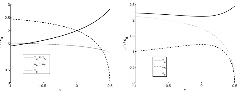
The zero eigenfrequencies in Eq. (12a) correspond to the rigid body motions. The eigenfrequencies (normalised with respect to h/cd) are plotted against Poisson’s ratio in Figure 1(left). It can be
seen that the largest eigenfrequency isω8for positive values ofν andω6=ω7for negative values
ofν. Note thatωmax=2cd/hforν=0 which, upon substitution into Eq. (1), leads to the
well-known rule-of-thumb that∆tcrit=“element size”/“wave speed”, although this rule-of-thumb must be applied with some safety factor for other values of Poisson’s ratio.
3.2. Three-noded equilateral triangle
The shape functions for a three-noded equilaterial triangle with heighthcan be written as
φ1=
h−x√3−y
2h (13a)
φ2=
h+x√3−y
2h (13b)
φ3=
y
−10 −0.5 0 0.5 0.5
1 1.5 2 2.5 3
ν
ω
h / c
d
ω4 = ω 5
ω6 = ω7
ω8
−10 −0.5 0 0.5
0.5 1 1.5 2 2.5
ν
ω
h / c
d
ω4
ω5
[image:7.595.101.497.64.216.2]ω6
Figure 1. Normalised eigenfrequenciesωh/cd against Poisson’s ratioν for square elements (left) and for right-angled isosceles elements (right)
where the origin of the Cartesian coordinate system has been chosen halfway the base of the triangle. The eigenvalue problem of Eq. (2) then becomes
ω6
h6(ω2
h2−9c2s
)2(
ω2
h2−9c2d+9c2s )
=0 (14)
which yields
ω2
1=ω22=ω32=0 (15a)
ω2
4=ω52=
9c2dq2
h2 (15b)
ω2
6=
9c2d(
1−q2)
h2 (15c)
Similar to the square element discussed above, it can be easily verified that the largest eigenfrequency isω4=ω5for negative Poisson’s ratios andω6for positive Poisson’s ratios.
3.3. Three-noded right-angled isosceles triangle
Although the equilateral triangle is probably the most regularly shaped triangle from a purely geometric point of view, it is also worthwhile to document the eigenfrequencies of a right-angled isosceles triangle since such elements would appear in structured meshes for rectangular domains. Taking the length of the hypothenuse to be equal to 2hso that the height of the triangle is againh, the shape functions can be written as
φ1=
h−x−y
2h (16a)
φ2=
h+x−y
2h (16b)
φ3=
y
h (16c)
The eigenvalue equation problem reads
ω6
h6(ω2
h2−6c2s ) (
ω4
h4−6ω2
h2c2d+27cd2c2s−27c4s )
=0 (17)
so that
ω2
1=ω22=ω32=0 (18a)
ω2
4=
6c2dq2
e
e
e e
e e
h
h
[image:8.595.193.373.75.180.2]α·h
Figure 2. Aspect ratio distortion for rectangular elements
ω2
5=
3c2d h2
(
1−
√
1−3q2(1−q2)
)
(18c)
ω2
6=
3c2d h2
(
1+
√
1−3q2(1−q2)
)
(18d)
The non-zero eigenfrequencies of Eqns. (18) are plotted against Poisson’s ratio in Figure1(right), and it can be seen thatω6is the largest eigenfrequency for all values ofν.
4. THE EFFECTS OF ASPECT RATIO DISTORTION ON RECTANGULAR ELEMENTS
The first type of element distortion that will be considered is denoted as “aspect ratio distortion” of rectangular elements. Applying aspect ratio distortion to a square, the dimensions of the (now rectangular) element can be indicated withhandα·h, respectively — see Figure2. Thus, α>1 sets the magnitude of aspect ratio distortion whilst maintaininghas the notation for the shortest distance within the element.
Including the aspect ratio parameter α into the evaluation of Eq. (2) results in a polynomial equation forωas
ω6h6(
3ω2h2α2
−4α2c2 d−4c
2 s
) (
3ω2h2α2
−4c2d−4α2c2 s
) (
ω2h2α2
−4α2c2 s−4c2s
)
× (ω4h4α2
−4ω2h2(α2+1)
c2d+64c2dc2s−64c4s )
= 0 (19)
which yields
ω12=ω22=ω32=0 (20a)
ω42=4c
2 d (
α2+q2)
3α2h2 (20b)
ω2
5=
4c2d(α2q2+1)
3α2h2 (20c)
ω2
6=
4c2 dq2
(
α2+1)
α2h2 (20d)
ω2
7=
2c2d
α2h2
(
α2+1
−
√
(α2+1)2
−16α2q2(1
−q2)
)
(20e)
ω2
8=
2c2 d
α2h2
(
α2+1+√(α2+1)2−16α2q2(1−q2)
)
(20f)
In Figure3the non-zero eigenfrequenciesω4–ω7are normalised with respect toω8and plotted
for a range of aspect ratiosαand a range of Poisson’s ratiosν. Since these ratios of eigenfrequencies are never larger than one, it can be concluded that ω8 as given in Eq. (20f) is the maximum
1 3 5 −1 −0.5 0 0.5 0 0.5 1 α ν ω4 / ω8 1 3 5 −1 −0.5 0 0.5 0 0.5 1 α ν ω5 / ω8 1 3 5 −1 −0.5 0 0.5 0 0.5 1 α ν ω6 / ω8 1 3 5 −1 −0.5 0 0.5 0 0.5 1 α ν ω 7 / ω 8
Figure 3. Rectangular elements: ratio of eigenfrequencies ω4/ω8 (top left), ω5/ω8 (top right), ω6/ω8 (bottom left) andω7/ω8(bottom right)
H H H H H H H H H H H H e e e b a h θ
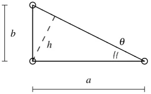
Figure 4. Aspect ratio distortion for right-angled triangular elements
5. THE EFFECTS OF ASPECT RATIO DISTORTION ON RIGHT-ANGLED TRIANGLES
Next, aspect ratio distortion is applied to right-angled triangles. The shortest distance within the triangle is the altitude from the right angle towards the hypothenuse, and this distance is kept constant ath. Several parametrisations are possible to capture this aspect ratio distortion, but the one that leads to the simplest expressions is that based on the angleθ depicted in Figure4. The coordinates of the triangle can then be quantified by the dimensionsa=h/sin(θ)andb=h/cos(θ) and the associated eigenvalue problem leads to the following polynomial equation:
ω6
h6(ω2
h2−6c2s ) (
ω4
h4−6ω2
h2c2d+27 sin2(2θ)(
c2d−c2s )
c2s )
=0 (21)
Therefore,
ω2
1=ω22=ω32=0 (22a)
ω2
4=
6c2dq2
h2 (22b)
ω2
5=
3c2d h2
(
1−
√
1−3 sin2(2θ)q2(1−q2)
)
[image:9.595.207.360.366.461.2]e
e
e
e e e
e
h
h
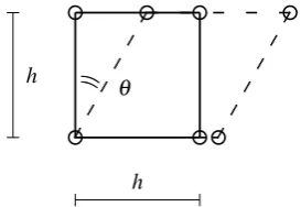
[image:10.595.220.357.81.175.2]θ
Figure 5. Angular distortion for rhombic elements
ω2
6=
3c2d h2
(
1+
√
1−3 sin2(2θ)q2(1
−q2)
)
(22d)
Since 0≤ q2 ≤ 34, the maximum value that ω 2
4 can attain is ω42 = 9c2d/2h2. Furthermore,
0≤q2(
1−q2)
≤ 14, so that the minimum value thatω 2
6 can attain is ω62=9c2d/2h
2. Therefore,
it can be concluded thatω4≯ω6. It is also clear thatω5≤ω6, thusω6is the largest eigenfrequency
for a right-angled three-noded triangle.
6. THE EFFECTS OF ANGULAR DISTORTION ON RHOMBIC ELEMENTS
Next, angular distortion is studied for square elements turning into rhombic-shaped elements. The main parameter of distortion is the change of the internal angles of the element, indicated withθas in Figure5. If the shortest distance of the element is to be kept constant ath, each edge of the element has lengthh/cos(θ). It is possible to express the shape functions directly in Cartesian coordinates, but this leads to lengthy and cumbersome derivations. More transparent expressions are obtained if isoparametric shape functions are formulated in the usual local coordinatesξ andη, which for rhombic shapes are related to the Cartesian coordinatesxandyviax=ξ/cos(θ) +ηtan(θ)and
y=η. The Jacobian matrix relating global to local coordinates only depends on the angleθand is thus constant throughout the element.
With these preliminaries, the eigenvalue problem of Eq. (2) reduces to
ω6h6(9ω4h4
−24ω2h2(
c2d+c2s )
+16 cos2(θ)(
c2d−c2s
)2
+64c2dc2s )
×
(
ω2h2
−8c2s ) (
ω4h4
−8ω2h2c2d+64 cos2(θ)c2dc2s−64 cos2(θ)c4s )
= 0 (23)
Accordingly, the eigenfrequencies of the element are given by
ω2
1=ω22=ω32=0 (24a)
ω42=4c
2 d
3h2
(
1+q2−(
1−q2)
sin(θ))
(24b)
ω52=4c
2 d
3h2
(
1+q2+(
1−q2)sin(θ))
(24c)
ω62=8c
2 dq
2
h2 (24d)
ω2
7=
4c2d h2
(
1−
√
1−4 cos2(θ)q2(1
−q2)
)
(24e)
ω2
8=
4c2d h2
(
1+
√
1−4 cos2(θ)q2(1−q2)
)
0 30 60 90 −1 −0.5 0 0.5 0 0.5 1 θ ν ω5 / ω8 0 30 60 90 −1 −0.5 0 0.5 0 0.5 1 θ ν ω 6 / ω 8
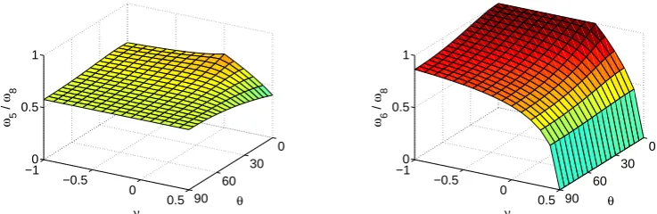
Figure 6. Rhombic elements: ratio of eigenfrequenciesω5/ω8(left) andω6/ω8(right)
Q Q Q Q Q Q Q Q Q e e e h
[image:11.595.191.405.232.327.2]α·h α·h
Figure 7. Angular distortion for isosceles triangular elements
The eigenfrequencies of Eqns. (12) are retrieved by takingθ=0.
With 0≤q2≤34 and taking 0≤θ ≤90◦, it can be stated thatω4≤ω5andω7≤ω8. In Figure
6the two eigenfrequenciesω5andω6are plotted normalised with respect toω8, which shows that
ω5<ω8andω6≤ω8. Therefore, the largest eigenfrequency isω8.
7. THE EFFECTS OF ANGULAR DISTORTION ON ISOSCELES TRIANGULAR ELEMENTS
Applying angular distortion to isosceles triangles is most conveniently done by taking the length of the longest side equal to 2αh, whereby the distortion parameterαis taken asα>1
3
√
3 in order to keep the shortest distance of the triangle equal toh(see Figure7). Including the angular distortion in the eigenvalue problem of Eq. (2) results in
ω6
h6(2ω2
h2α2
−3(3α2+
1)c2s ) (
2ω4
h4α2
−3ω2
h2(3α2+
1)c2d+54cd2c2s−54c4s )
=0 (25)
which leads to
ω2
1=ω22=ω32=0 (26a)
ω2
4=
3c2d(3α2+1)
q2
2α2h2 (26b)
ω2
5=
3c2d
4α2h2
(
3α2+1
−
√
(3α2+1)2−48α2q2(1−q2)
)
(26c)
ω2
6=
3c2d
4α2h2
(
3α2+1+√(3α2+1)2−48α2q2(1−q2)
)
(26d)
Figure 8depicts the ratio of ω4 divided byω6 for a range of values for the distortion parameter
α and the Poisson’s ratioν, and it can be verified thatω4≤ω6. Furthermore, from Eqns. (26) is
it clear thatω5≤ω6. Therefore, the largest eigenfrequency for a three-noded isosceles triangle is
1
3
5 −1
−0.5 0
0.5 0
0.5 1
3 α2
ν ω 4
/
[image:12.595.219.380.71.186.2]ω 6
Figure 8. Isosceles triangles, ratio of eigenfrequenciesω4/ω6
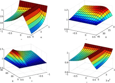
8. COMPARING DISTORTED AND UNDISTORTED ELEMENTS
Now that the maximum eigenfrequencies of the distorted elements have been determined, it is of interest to compare these to the maximum eigenfrequencies of the associated undistorted elements. Since the shortest distance in all expressions for the eigenfrequencies has been denoted by h
throughout, it can be verified whether element distortion has an adverse or beneficial effect on the maximum eigenfrequency.
The quantity of interest is the maximum eigenfrequency of the distorted element divided by the maximum eigenfrequency of the corresponding undistorted element. In particular,
• For aspect ratio distortion of quadrilaterals,ω8from Eq. (20f) is divided byω6from Eq. (12c)
orω8 from Eq. (12d), as appropriate. The result is plotted in Figure9, top left. It can be
verified that the maximum eigenfrequency of a rectangle is never larger than the maximum eigenfrequency of a square with identical shortest distance.
• For aspect ratio distortion of right-angled triangles,ω6from Eq. (22d) is divided byω6from
Eq. (18d). The result is plotted in Figure9, top right. In this case, element distortion does lead to an increase of the maximum eigenfrequency, but this increase is relatively small. The largest increase equals 2/√3≈1.155 which occurs for the hypothetical combination of Poisson’s ratioν=0 and distortion angleθ =0. However, if one imposes a bound on the maximum acceptable distortion during mesh generation (that is, an upper bound on the ratioa/b, or a lower bound on angleθ), the largest increase in the eigenfrequency would be less than 2/√3.
• For angular distortion of quadrilaterals,ω8 from Eq. (24f) is divided byω6 from Eq. (12c)
orω8from Eq. (12d), as appropriate. The result is plotted in Figure9, bottom left. Also in
this case, element distortion leads to a modest increase in the maximum eigenfrequency. The largest increase equals√2 and is obtained for the limit case of degenerate element geometry via distortion angleθ=90◦combined with Poisson’s ratioν=0. Again, this type of distortion
can be controlled during mesh generation so that increase factors lower than√2 will then be obtained.
• For angular distortion of isosceles triangles,ω6 from Eq. (26d) is divided byω4 from Eq.
(15b) orω6from Eq. (15c), as appropriate. The result is plotted in Figure9, bottom right. As
can be seen, the maximum eigenfrequency of a distorted isosceles triangle is never larger than the maximum eigenfrequency of an equilateral triangle with identical shortest distance.
1
3
5 −1
−0.5 0
0.5 0.7
0.8 0.9 1
α ν
0 15 30 45 −1
−0.5 0
0.5 0.8
1 1.2
θ ν
0 30 60 90
−1 −0.5 0
0.5 0.5
1 1.5
ν θ
1
3
5 −1
−0.5 0
0.5 0.6
0.8 1
3 α2
[image:13.595.112.481.67.331.2]ν
Figure 9. Maximum eigenfrequencies of distorted elements divided by those of undistorted elements — aspect ratio distortion of square elements (top left) and right-angled triangles (top right); angular distoration
of square elements (bottom left) and isosceles triangles (bottom right)
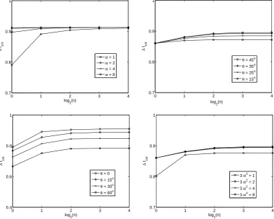
9. CRITICAL TIME STEP FOR FINITE ELEMENT ASSEMBLIES
Next, finite element assemblies of more than one element will be considered. As mentioned in the Introduction, most researchers estimate the critical time step by focussing on a single element, but according to Eq. (1) the exact value of the critical time step is found by computing the eigenfrequencies of the entire finite element mesh, not of a single element in isolation — although the latter gives a safe bound to the exact (globally obtained) value of the critical time step [3].
Structured patches of multiple finite elements are generated by taking n elements in each direction. For quadrilaterals, this means that n×nelements with identical dimensions are used. For triangles, each of the quadrilaterals is then subdivided into two triangles with identical dimensions (thus leading ton×n×2 elements in total). As such, patches of distorted right-angled triangles and patches of distorted isosceles triangles are generated from initial grids of rectangles and parallelograms, respectively. Values forn∈[1,2,4,8,16]are taken, and global stiffness and (lumped) mass matrices are generated using mass densityρ =1 kg/m3, Young’s modulusE=1
N/m2and Poisson’s ratioν= 1
4. The eigenfrequencies of the resulting system are then obtained in
numerical (rather than symbolic) format and substituted into Eq. (1) to obtain the critical time step. In Figure10the critical time steps are plotted for the two types of elements and the two types of element distortion that are studied, using a range of element distortion parameters. It can be seen in all considered cases that larger patches of elements lead to larger values of the critical time step, although there seem to be asymptotic values for each combination of element type and distortion type. The main observations of Section 8 are also confirmed, namely that increased
0 1 2 3 4 0.7
0.8 0.9 1
log
2(n)
∆
tcrit
α = 1
α = 2
α = 4
α = 8
0 1 2 3 4
0.7 0.8 0.9 1
log
2(n)
∆
tcrit
θ = 45o
θ = 35o
θ = 25o
θ = 15o
0 1 2 3 4
0.4 0.6 0.8 1
log
2(n)
∆
tcrit
θ = 0
θ = 15o
θ = 30o
θ = 60o
0 1 2 3 4
0.7 0.8 0.9 1
log
2(n)
∆
tcrit
[image:14.595.99.497.71.388.2]3 α2 = 1 3 α2 = 2 3 α2 = 4 3 α2 = 8
Figure 10. Critical time step∆tcritversus number of elementsn— rectangular elements (top left), right-angled triangles (top right), rhombic elements (bottom left) and isosceles elements (bottom right)
10. CONCLUSIONS
The effects of element distortion on the critical time step of low-order, two-dimensional finite elements has been studied in this paper, with focus on aspect ratio distortion and angular distortion of linear triangles and bilinear quadrilaterals. The dynamic eigenvalue problem has been formulated and solved on element level for a number of cases, and the maximum eigenfrequencies have been identified in symbolic form making use of appropriate parameters to capture the element distortion such as aspect ratio or change of internal angle. Thus, the maximum eigenfrequencies were found in terms of material parameters (dilatational wave speed and Poisson’s ratio), the shortest distance within the element, and the element geometry.
The overriding conclusion is that element distortion can have an adverse effect on the critical time step, nevertheless such effects tend to be limited. In many cases there was in fact a slightbeneficial
effect of element distortion (that is, the critical time step was found to be increased by element distortion), whereas the most significant decrease of the critical time step was found to be a factor of√2. Thus, the rule-of-thumb used in practice that the critical time step equals the shortest distance divided by the dilatational wave speed, with a modest safety factor, can still be used.
here, but they can be verified using the characteristic polynomials presented in AppendicesAand
B, respectively.
ACKNOWLEDGEMENTS
Financial support from the Royal Society under International Joint Project “Bipenalty method for finite elements and explicit time integration” is gratefully acknowledged.
REFERENCES
1. Ling X, Cherukuri H. Stability analysis of an explicit finite element scheme for plane wave motions in elastic solids.
Computational Mechanics2002;29:430–440.
2. Hughes T.The finite element method: linear static and dynamic finite element analysis. Prentice-Hall, 1987. 3. Lin J. An element eigenvalue theorem and its application for stable time steps.Computer Methods in Applied
Mechanics and Engineering1989;73:283–294.
4. Flanagan D, Belytschko T. Eigenvalues and stable time steps for the uniform strain hexahedron and quadrilateral.
ASME Journal of Applied Mechanics1984;51:35–40.
5. Belytschko T, Lin J. Eigenvalues and stable time steps for the bilinear Mindlin plate element.International Journal for Numerical Methods in Engineering1985;21:1729–1745.
6. Lin J. Bounds on eigenvalues of finite element systems. International Journal for Numerical Methods in Engineering1991;32:957–967.
7. Benson D. Stable time step estimation for multi-material Eulerian hydrocodes. Computer Methods in Applied Mechanics and Engineering1998;167:191–205.
8. Koteras J, Lehoucq R. Estimating the critical time-step in explicit dynamics using the Lanczos method.
International Journal for Numerical Methods in Engineering2007;69:2780–2788.
9. Nakamachi E, Huo T. Dynamic-explicit elastic plastic finite-element simulation of hemispherical punch-drawing of sheet metal.Engineering Computations1996;13:327–338.
10. Chung W, Cho J, Belytschko T. On the dynamic effects of explicit FEM in sheet metal forming analysis.
Engineering Computations1998;15:750–776.
11. Kim J, Kang SJ, Kang BS. A comparative study of implicit and explicit FEM for the wrinkling prediction in the hydroforming process.International Journal of Advanced Manufacturing Technology2003;22:547–552.
12. van den Boogaard A, Hu´etink J. Simulation of aluminium sheet forming at elevated temperatures.Computer Methods in Applied Mechanics and Engineering2006;195:6691–6709.
13. Wang Z, Zeng S, Yang X, Cheng C. The key technology and realization of virtual ring rolling.Journal of Materials Processing Technology2007;182:374–381.
14. Aguinaga I, Fierz B, Spillmann J, Harders M. Filtering of high modal frequencies for stable real-time explicit integration of deformable objects using the finite element method.Progress in Biophysics and Molecular Biology
2010;103:225–235.
15. Olovsson L, Unosson M, Simonsson K. Selective mass scaling for thin walled structures modeled with tri-linear solid elements.Computational Mechanics2004;34:134–136.
16. Hetherington J, Askes H. Penalty methods for time domain computational dynamics based on positive and negative inertia.Computers and Structures2009;87:1474–1482.
17. Askes H, Caram´es-Saddler M, Rodr´ıguez-Ferran A. Bipenalty method for time domain computational dynamics.
Proceedings of the Royal Society A2010;466:1389–1408.
18. Hetherington J, Rodr´ıguez-Ferran A, Askes H. A new bipenalty formulation for ensuring time step stability in time domain computational dynamics.International Journal for Numerical Methods in Engineering2012;90:269–286.
19. Hetherington J, Rodr´ıguez-Ferran A, Askes H. The bipenalty method for arbitrary multipoint constraints.
International Journal for Numerical Methods in Engineering2013;93:465–482.
20. Macek R, Aubert B. A mass penalty technique to control the critical time increment in explicit dynamic finite-element analysis.Earthquake Engineering and Structural Dynamics1995;24:1315–1331.
21. Olovsson L, Simonsson K, Unosson M. Selective mass scaling for explicit finite element analyses.International Journal for Numerical Methods in Engineering2005;63:1436–1445.
22. Plech´aˇc P, Rousset M. Implicit mass-matrix penalization of Hamiltonian dynamics with application to exact sampling of stiff systems.Multiscale Modeling and Simulation (SIAM)2010;8:498–539.
23. Askes H, Nguyen D, Tyas A. Increasing the critical time step: micro-inertia, inertia penalties and mass scaling.
Computational Mechanics2011;47:657–667.
24. Olovsson L, Simonsson K. Iterative solution technique in selective mass scaling.Communications in Numerical Methods in Engineering2006;22:77–82.
25. Lombardo M, Askes H. Lumped mass finite element implementation of continuum theories with micro-inertia.
International Journal for Numerical Methods in Engineering2013;96:448–466.
A. CHARACTERISTIC POLYNOMIALS FOR QUADRILATERAL ELEMENTS: SELECTIVE REDUCED INTEGRATION
Selective reduced integration implies that the shear terms are under-integrated. This can be achieved by evaluating the third row ofBas given in Eq. (9) at the centre of the element only. For four-noded square elements, the eigenvalue problem of Eq. (2) then reads
ω6h6(
3ω2h2
−4c2d)2(
ω2h2
−8c2s)2(
ω2h2
−8c2d+8c2s)
=0 (27)
The eigenvalue problem for a rectangular element with selective reduced integration can be written as
ω6h6(
3ω2h2
−4c2d) (
3ω2h2α2
−4c2d) (
ω2h2α2
−4α2c2 s−4c2s
)
× (ω4h4α2
−4ω2h2(
α2+1)
c2d+64c2dc2s−64c4s )
= 0 (28)
and for a rhombic quadrilateral element it reads
ω6h6(
9ω4h4
−24ω2h2c2
d+16 sin 2(2θ)c2
dc2s−16 sin2(2θ)c4s+16 cos2(θ)c4d )
×
(
ω2h2
−8c2s) (ω4h4
−8ω2h2c2
d+64 cos2(θ)c2dc2s−64 cos2(θ)c4s )
= 0 (29)
B. CHARACTERISTIC POLYNOMIALS FOR QUADRILATERAL ELEMENTS: REDUCED INTEGRATION
If reduced integration is applied to all three rows of matrixB, the eigenvalue problem of Eq. (2) for a four-noded square element reduces to
ω10h10(
ω2h2
−8c2s)2(
ω2h2
−8c2d+8c2s)
=0 (30)
Applying reduced integration to a rectangular element yields
ω10h10(
ω2h2α2−4α2c2s−4c2s) (
ω4h4α2−4ω2h2(
α2+1)
c2d+64c2dc2s−64c4s)
=0 (31)
and for a rhombic element this gives
ω10
h10(ω2
h2−8c2s ) (
ω4
h4−8ω2
h2c2d+64 cos2(θ)cd2c2s−64 cos2(θ)c4s )
=0 (32)