This is a repository copy of
Social Institutions and Economic Inequality Modeling the onset
of the Kuznets Curve
.
White Rose Research Online URL for this paper:
http://eprints.whiterose.ac.uk/89324/
Version: Accepted Version
Proceedings Paper:
Alvarez-Pereira, B, Bale, CSE, Alves Furtado, B et al. (4 more authors) (2014) Social
Institutions and Economic Inequality Modeling the onset of the Kuznets Curve. In:
MacKerrow, E, Terano, T, Squazzoni, F and Sichman, JS, (eds.) Proceedings of the 5th
World Congress on Social Simulation. 5th World Congress on Social Simulation, 04-07
Nov 2014, Sao Paulo, Brazil. . ISBN 978-0-692-31895-9
eprints@whiterose.ac.uk https://eprints.whiterose.ac.uk/
Reuse
Unless indicated otherwise, fulltext items are protected by copyright with all rights reserved. The copyright exception in section 29 of the Copyright, Designs and Patents Act 1988 allows the making of a single copy solely for the purpose of non-commercial research or private study within the limits of fair dealing. The publisher or other rights-holder may allow further reproduction and re-use of this version - refer to the White Rose Research Online record for this item. Where records identify the publisher as the copyright holder, users can verify any specific terms of use on the publisher’s website.
Takedown
If you consider content in White Rose Research Online to be in breach of UK law, please notify us by
Social Institutions and Economic Inequality
Modeling the onset of the Kuznets Curve
Brais Alvarez-Pereira1, Catherine Bale2, Bernardo Alves Furtado3, James E. Gentile4, Claudius Gr¨abner5, Heath Henderson6, and Francesca Lipari7
1
European University Institute
2
Centre for Integrated Energy Research, University of Leeds
3
Institute for Applied Economic Research and CNPq
4
The MITRE Corporation⋆⋆
5
Institute for Institutional and Innovation Economics, University of Bremen
6
Inter-American Development Bank
7
University of Tor Vergata
Abstract. Theoretical models of the Kuznets Curve have been purely analytical with little contribution to the timing of the process and to the presence of additional mechanisms affecting its timing. This paper proposes an agent-based version of Acemoglu and Robinsons model of the political economy of the Kuznets Curve. In extending their analytical framework we include heterogeneity of agents’ income and a mating mechanism that together represent elements of social mobility. These two simple changes proved to be enough to shed light on the length and timing before high inequality implies regime change. Thus, this work may contribute to an effective empirical assessment of the Kuznets curve as it explicitly considers the time dimension of the process and the effects of considering social dynamics.
1
Introduction
In 1955 Simon Kuznets hypothesized that there exists an inverse U-shaped pattern in long-run processes of economic development [12]; that is, economic inequality increases as an economy develops, before decreasing after a certain level of income is reached. Although the hypothesis has been subjected to extensive examination, there remain many open questions in relation to this theory. In particular, these questions relate to: a) evidence for the theory’s empirical validity; b) theory explaining why the curve arises; and c) shape and onset of the curve in different countries.
In their 2002 paper, Acemoglu and Robinson [2] (AR) offer a political economy theory of the Kuznets Curve. They propose that ”capitalist industrialization tends to increase inequality, but this inequality contains the seeds of its own destruction,
⋆⋆
because it induces a change in the political regime toward a more redistributive system” [2, p. 184]. In contrast to other theories they argue instead that political factors and institutional change are crucial. They model redistribution and the associated reduction in inequality as a process where poor agents force political instability and the political elites extend redistribution through taxation to avoid a revolution. Society, therefore, moves from an autocratic to a democratic regime.
However, they make several unrealistic assumptions in their analytical model and do not consider the dynamics of the Kuznets Curve explicitly. In this paper, we take their paper as a starting point and formalize their interpretation of the Kuznets Curve in an agent-based model. This allows us to explore the effects of relaxing some of the assumptions made on the shape and onset of the Kuznets curve and to consider the time dimension explicitly. Specifically, we extend the model to include heterogeneity in the agents (both poor and rich) by allowing for an income distribution, and we include also a mating mechanism that allows mobility between the two classes, rich and poor, via the social institution of marriage.
The paper is structured as follows. In section 2 we present an overview of the current literature highlighting gaps in the theory, and consider the discussion related to the existing empirical evidence on the Kuznets Curve. In section 3 we develop the model, showing both the features that we reproduce and those we introduce as novel. Section 4 covers assumptions and special cases. Section 5 describes the implementation of the agent-based model. Section 6 presents the parameterization, a brief sensitivity analysis and the results. We conclude the paper in section 7.
2
Literature survey
In his original paper, Kuznets [12] used time series data for England, USA and Germany for the formulation of his stylized facts about the dynamics of growth and inequality, namely an increasing inequality for early stages of development (i.e. for aprox. 50 years) and a shrinking inequality thereafter. He expected the then underdeveloped countries to follow a similar pattern. He was, however, skeptical of the quality of his data set and pointed out that ”the results [can be] considered as preliminary informed guesses” [12, p. 4].
Theoretical contributions The motivation for theoretical models yielding a Kuznets relationship is the belief that empirical regularities as such (if they exist) can only be interesting to the extent that ”they can be viewed as providing some clues to the mechanisms through which the development process affects the degree of inequality” [3, p. 338]. If such deeper mechanisms could be identified, reasonable policy advice could be derived from the observations, a goal that has been articulated throughout the entire literature on inequality.
The first important theoretical contribution is the paper of Lewis [13] in which he coined the idea of dualistic development, i.e. the coexistence of two sectors with important differences in at least one relevant dimension, mostly productivity. In this paper, the author used the example of a capitalist and a subsistence sector and as capital is only used in the first sector, it has a higher output per head and higher wages. If more capital is produced, more workers move from the subsistence to the capitalist sector and their income rises. Kuznets idea of the population shift from agricultural to urban employment was certainly inspired by this paper. The dualistic development models were further extended and refined in further papers by Ranis and Fei (1961), Harris and Todaro (1970), and Anand and Kanbur (1993).
An important step was the work of Robinson [15] who provided a more formal two-sector model that deals with the inequality dynamics explicitly and considers different income distributions in the sectors and a shift of the relative population of one sector. He showed that such a setting will frequently produce a Kuznets pattern. These theoretical considerations have been used to justify a great set of policy measures.AR, while building on previous work in the political science literature are the first who propose a political economy explanation for the Kuznets curve.
Empirical contributions The empirical assessment of the Kuznets curve has been characterized mainly by discussions about the quality of data and the choice of estimation techniques. Although Kuznets himself used time series data for the formulation of his theory, the vast majority of empirical work until recently has focused on cross-sectional data , simply because other data was not available [3, p. 307].
The most famous papers of the early era concluded with support for the Kuznets relationship and triggered a huge policy debate [3]. Later, Anand and Kanbur [5] took these papers as a starting point for their critique of the Kuznets concept and highlighted the insufficient data and the lack of consensus about the adequate estimation techniques. Until 1998, studies used exclusively cross-sectional data and the resulting evidence was mixed, with a tendency to be negative ([10], [14]). But the overall explanatory power of these cross-sectional studies has frequently been questioned. The Kuznets hypothesis is about how inequality develops within one country, not how it develop across countries, what is tested if one relies on cross sectional data.
this first panel data set, a new wave of empirical studies about the Kuznets Curve emerged. While DS find a statistically significant Kuznets-like relationship for a pooled regression, they reject the presence of the Kuznets Curve when they use fixed effects estimation. Savvides and Stengos (2000) using a threshold regression model did not find evidence for the Kuznets relationship (or any other well-defined relation) either and Higgins and Williamson (1999) found evidence for the curve only if they controlled for demographic and globalization effects. Many authors used the data set to argue for the importance of additional mechanisms such as policies and openness, thereby rejecting the idea of an unconditional relationship and explaining the resulting differences across countries ([16], [8]). Later, the data set provided by DS received heavy critique for including inconsistent inequality measures and providing in-accurate time series [6]. After this, almost no study was published using the original data set any more. In contrast to earlier praxis, some non-parametric studies were conducted using a refined version of the DS data set, finding mixed evidence. Another issue not adequately dealt with in the empirical literature is the time period over which the Kuznets Curve develops: The existing theoretical contributions do not make concrete statements about the time horizon of the Kuznets curve. Because of data scarcity most studies assessed a time span of at most 40 years.
We conclude that the evidence for the Kuznets curve is very mixed. While the evidence from cross-sectional studies cannot be trusted, more recent studies suggest that Kuznets patterns can be observed in some individual countries, which suggests an important role for country and region specific influences. There has never been a trustworthy study considering the Kuznets curve over more than 60 years, and considerations about data quality and adequate estimation techniques are not yet fully resolved.
3
The theoretical model
Environment As in the original model [2] we consider an infinite-horizon non-overlapping generation model in which parents invest in their offspring’s education. In the benchmark model, a discrete population ofN agents is divided in two groupsNr
t andN p
t, respectively, the total number of rich and poor agents in periodt. In every period, every agent in the population meets another agent, which might or not be from the same social class, and they beget two children. It is assumed that 1/2< N0p/(N0p+Nr
0)<1 so that rich agents are a minority elite in the beginning. Political power is initially concentrated in the hands of the elite, where decisions will be taken by the median voter.
The final good is produced by each agent using a linear technology. Individuals can choose to allocate their capital between the formal sector, using a market technology yim
t =Ahimt , and the informal sectoryibt =Bhibt , wherehimt is the amount of capital used in the formal sector or market production by agentiin periodtand hib
t is the amount of capital he devotes to informal production. In the modelA > B, so production in the formal sector is always more productive. Production in the informal sector has the advantage of being untaxed. The relation betweenAandB will determine the maximum possible tax.
Aside from the heterogeneity of the agents, this formalization is the same as that of AR [2].
Mating The mating mechanism is not included in the original paper. We consider two agents in the populationi, j∈ {r, p} who select each other in order to form a family. We denote the total probability of an agenti mating another agentj asPii
t . If mating is perfectly random, for a large N the probability of a poor agent mating with a poor agent isλt=Ntp/(N
p
t +Ntr). If mating is perfectly assortative the probability of a poor agent mating with a poor agent is unity. We define such probability as: Ptpp = λt+α(1−λt) = α+λt(1−α) where
α is a measure of assortativity. Hence, when α = 0, random mating results, while forα= 1, mating is perfectly assortative. Following the same logic, given 1−λt=Ntr/(N
p
t +Ntr), the probability of a rich agent mating with a rich agent is simply given byPrr
t = (1−λt) +αλt= 1−λt(1−α)
The remaining probabilities are easily computed asPtpr= (1−α)(1−λt) and
Ptrp= (1−α)λt. αis then our inter-class mating parameter (assortativity). In every periodtthe expected number of poor agents that mate outside their class isNtpP
pr t =N
p
t[1−(α+λt(1−α))]. The expected number of rich agents that mate outside their class isNr
tP rp
t =Ntr[1−(1−λt(1−α))]. It is easy to see that expected values match.
The consumption-investment decision When two agents mate they become a family, for which the total amount of wealth or final good is the sum of the individual . For familyz, made up of agentsiandj ytf =yit+y
j
t, where for a generic agenti,yi
t=ytim+ytib; this holds also for the agentj and, in principle, is expression of both formal, m, and informal,b sector.
We assume that both parents are altruistic towards their children, regardless their social origin. Accordingly, the decision about how much of the final good to consume and how much to invest on the children education is jointly taken between the two members of the family,ez
t+1, following preferences,
uz(cz
t, ezt+1) =
(cz
t)1−γ(ezt+1/2)γ ifeft+1z >2 (cz
t)1−γ ife f t+1z≤2
(1)
where γ ∈ (0,1) , cz
t is the joint consumption of the parents in period t, andez
children, and so the utility function implies that a family will invest in education if and only if the amount they can dedicate to this is larger than 2 (1 for each of the children). Hence, the investment in offspring education will be
ez t+1=
γyˆtf ifγyˆz t >2 0 ifγyˆz
t ≤2
(2)
For each new child,k, his human capital is given by
hkt+1=max{1;Z(ezt+1/2)β}, (3)
withZ >1 andβ <1. This guarantees that accumulation of capital does not continue indefinitely. Notice also that equation (3) guarantees that the minimum amount of capital is 1.
Taxes and transfers No matter how forward-looking the parents would be for their children, their investment decision depends on the tax regime. We assume that taxes cannot be made person-specific and so they are proportional to the amount of market-produced good. However, we have introduced the family unit as agent performing the investment and voting decisions, then, for every family, post-tax total income is simply ˆyz
t = (1−τt)Ahtzm+Tt+ytzb which simplifies to
ˆ
ytz= (1−τt)Ahzmt +Tt (4)
if both parents produce all of their final goods in the formal sector. This will be the case in equilibrium.τt is the tax rate andTt, the transfer in each period, is just given by
Tt=
PN
i=1ytzm
N . (5)
The government’s budget constraint is given byN Tt=τtAHtm, whereHtm=
Pm
i=1himt is the total production in the formal sector of the economy. Initially the tax rate will be set by the median voter among rich agents. However, poor agents can overthrow the existing government and take over the capital stock at any periodt. We assume that a revolution is triggered when more than half of the population are materially better off than under the government of the rich elite. If it is triggered, a revolution always succeeds, with a proportion 1−µof the capital stock being destroyed, and the remaining of it being shared equally among the whole population. Therefore,µindicates how costly the revolution would be. Hence, if there is a revolution at periodt, each family receives
yzt =
µAHt
N (6)
For the median rich agent it will always be preferable to extent the franchise and open the regime to democracy than to let the revolution happen (see section 4). Hence, if the revolution constraint binds at any given period, the elite will introduce democracy, allowing the whole population to vote. The equilibrium tax rate in the first democratic period will be
ˆ
τ= A−B
A , (7)
the maximum tax level which does not imply agents allocating their capital to production in the informal level. The timing of the model in each period is as follows:
1. Parents die and the new generation receive education bequests. Upon receiving the bequest, the new generation makes a marriage decision. Social mobility can be improved by marriage.
2. The median voter among the rich agents sees everybody’s capital endowment and finds out if a revolution is optimal for half of the population or more, in which case he will choose to extend the franchise and open the regime to democracy.
3. If the franchise has been extended, family, the two parents, decide if they prefer to vote and select the optimal tax level or to support a revolution, which never happens in equilibrium.
4. Each family allocates his capital stock between formal sector and informal sector production and the family’s consumption and bequest levels.
4
Analysis
In this section we comment on the model assumptions and the case we choose for the simulation.
For the assumptions of the model the reader is referred to AR[2]. The main assumptions we keep are: the zero bequest assumption, the steady state assump-tion, the fact that median rich agent prefers democracy to revoluassump-tion, and initial conditions which ensure that rich agents who marry other rich agents are able to accumulate capital when there are not taxes. These conditions imply that poor agents cannot accumulate wealth even in the absence of taxes, while economic growth exists in the economy because rich agents start with less than steady state human capital, and are able to accumulate wealth until they reach the steady state level.
extended when wealth under autocracy becomes lower for at least half of the population than what they would get after a revolution. Increasing inter-class mating has two effects: On the one side it increases economic growth, on the other it decreases inequality. When a rich agent and a poor agent together create a rich family, the case chosen for our experiment, inter-class mating decreases social inequality and increases economic growth. Then, the effects of introducing inter-class mating (α <1) in an environment in which the franchise would be extended at a certain periodt=kwill be either:
1. To modify the time for a revolution to be optimal for at least half of the pop-ulation, depending on whether the growth or the inequality effect dominates. Our simulations suggest a domination of the growth effect, by increasing the number of families which are able to accumulate wealth, increasing inter-class mating increases total wealth in the autocratic regime, making the revolution optimal for the poor proportion of the population earlier in time.
2. If inter-class mating is high enough, it might prevent the revolution constraint from ever being triggered. Since we are assuming the median voter of the rich takes the political decisions, democracy arrives just because all agents become rich at some point.
Democracy When democracy is trivially reached because everybody becomes rich or because everybody becomes poor, then there will be no taxes, and consequently no political decision is taken. If democracy is reached through the revolution, the median voter will choose the maximum possible tax rate in the first democratic period. After this, inter-class mating and redistributive taxes will decrease inequality. At some point, it might occur that the median voter is not interested in positive taxes anymore. Formally, he chooses τ as to optimize:
τm∈Argmax (1−τt)Ahmt +
τmY t
N (8)
So the optimal tax level is simply given by:
τm=
0 ifAhm t > YNt
(A−B)
A if otherwise
(9)
In the next section, we consider the implementation of the theoretical model as an agent-based model.
5
Model Implementation
1. Each agent calculates post-tax income as (1−τ)Aw+rwherewis wealth andris the transfer.
2. Each agent computes its savings as savings rate time post tax income. 3. A regime choice is made. If the richest poor agent’s potential income
un-der democracy (µAHt/Np) is greater than its current post-tax income, the democracy is set and democracy continues through the execution.
4. If democracy is the current regime, the median agent, sorted by wealth, sets the tax rate. The rate is zero if this agent has above average wealth or (A−B)/Aotherwise.
5. Transfers are calculated asr=τ A/N.
6. In assortative mating, agents were paired based on the assortative parameter and a new generation was generated where two ‘parents’ begat two ‘children’. The children wealth were set as the average between their parent’s savings. Each agent is classified as rich or poor depending on their wealth relative to the poverty line.
7. In one-to-one mating, each agent generates a ‘child’ and its savings are passed down.
8. This generation is processed just as in steps 1–8.
6
Results and Discussion
[image:10.612.135.516.466.623.2]Parameterization and Sensitivity Analysis Where possible, we use empir-ical data to inform the model parameterization. Some parameters are derived from the same equations as given in AR, the remaining parameters were set explicitly. Table 1 shows the origin of the parameters and values used in the baseline scenario. In all runsN = 1,000 andH = 1,000.
Table 1.Parameter Values
Parameter Baseline Origin
Gini Coefficient 0.10 Informed by data [7]
δ: Lorenze curve parameter 0.82 Derived from other parameters
∆: % of poor 0.99 Model initial condition
I: Threshold agent 990 Derived from other parameters
Hm: Threshold agent (90th percentile) 1.87 Derived from other parameters
A: Parameter on modern sector production function 2.67 Derived from other parameters
B: Parameter on informal sector production function 2.13 Derived from other parameters
γ: Savings rate 0.20 Informed by data [7]
Z: Parameter on ospring human capital function 3.37 Set as initial condition
β: Exponent on ospring human capital function 0.75 Set as initial condition
µ: Proportion of economy remaining after revolution 0.85 Set as initial condition
τ: Tax rate 0.20 Informed by data [7]
the share of savings imposed to the economy determine the value of productivity on the formal sector. Derived from that, the equations provide the productivity on the informal sector. Forδclose to 1 and derived productivity much higher than empirically observed, inequality rises for all values ofα. The model also allows for a variation in the size of the economy that is left after a revolution. Results vary little with most distributions showing an increase in inequality followed by a short decrease before simulation is stopped with no more poor agents.
All considered the sensitivity analysis showed that the model is robust to transformations in the parameters as long as they are within the constraints and conditions imposed by the construction of the model itself.
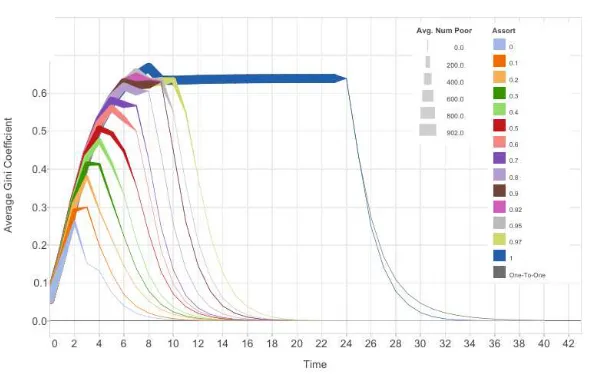
[image:11.612.135.430.385.574.2]Results Figure 1 presents the results associated with the baseline parameteri-zation. For alternative values ofα, we plot the time series of income inequality and poverty. Income inequality is measured by the Gini coefficient and poverty is captured by the number of poor agents. Recall that α = 0 corresponds to perfectly random mating,α= 1 corresponds to perfectly assortative mating, and a unit of time corresponds to a generation. Three interesting conclusions emerge from Fig. 1: higher assortativity in mating is associated with (1) a later onset of the Kuznets curve; (2) greater inequality; and (3) an increased persistence of poverty.
Fig. 1.Results. The Figure shows the evolution of the Gini coefficient for α= 0 to
α = 1 (i.e. from random to perfectly assortative mating). The width of the line is proportional to the number of poor agents at a given time step.
all intermediate values ofαreveals that the turning point increases monotonically with assortativity in mating. The second conclusion follows immediately from the first: for those values ofαthat correspond to a later onset of the Kuznets Curve we see that higher levels of inequality are obtained. Specifically, we see that for α = 1 peak inequality nearly reaches 0.70 whereas for α = 0 peak inequality remains relatively low at approximately 0.25. Analogous to the first conclusion, it is then evident that peak inequality increases monotonically in the assortativity of mating. With respect to the third conclusion, it is evident that for greater values ofαpoverty appears more persistent. That is, forα= 1 a non-negligible quantity of agents remain impoverished untilt = 23 whereas forα= 0 poverty is nearly completely eradicated byt= 2. Thus, in examining all intermediate values ofαwe see that the third conclusion echoes that of the first and second: we see yet another monotonic relationship as the duration of poverty is increasing in α. Regarding intuition, first consider the case where α= 1. In this scenario, marriage induces no social mobility and redistribution can only occur with taxation under democracy. For a given parameterization, the revolution constraint dictates that the franchise will be extended when per capita wealth (i.e.H/Hp) is sufficiently greater than the wealth of the wealthiest poor agent. The model outcomes forα= 1 thus depend primarily on the growth rate of the economy relative to that of the wealthiest poor agent. When α= 0, social mobility manifests through interclass marriage, which exerts influence on the transition to democracy. From Fig. 1, we see that this case is characterized by an immediate reduction in the number of poor agents, which exerts upward pressure on per capita wealth through both decreasing Hp and increasingH. This phenomenon leads to a more rapid transition to democracy and thus the earlier onset of the Kuznets curve. For 0< α <1 we observe that the higherα, the longer the Kuznets process lasts.
7
Conclusion
The second contribution is of a methodological kind. Our model takes a purely analytical model as a starting point, replicates the behavior of this model in an agent-based simulation, and then relaxes some of the assumptions required to keep the original model tractable. So it allows the consideration of the dynamics explicitly. While there are only a few models of this kind (e.g. [4] and [11] for the standard general equilibrium model), our model illustrates the usefulness of this approach. The rigor of the previous analytical model is sustained, but in our approach we are able to go beyond its application and assess its sensitivity to the rigid assumptions previously made. Our agent-based model will allow for further exploration of the factors affecting the timing and onset of the Kuznets Curve, and can also be applied to understand economic inequality in different countries with different levels of social mobility.
References
1. PEKC model.http://jegentile.github.io
2. Acemoglu, D., Robinson, J.A.: The political economy of the kuznets curve. Review of Development Economics 6(2), 183–203 (2002)
3. Ahluwalia, M.S.: Inequality, poverty and development. Journal of Development Economics 3(4), 307–342 (1976)
4. Albin, P., Foley, D.K.: Decentralized, dispersed exchange without an auctioneer: A simulation study. Journal of Economic Behavior & Organization 18(1), 27 – 51 (1992)
5. Anand, S., Kanbur, S.: Inequality and development. a critique. Journal of Develop-ment Economics 41(1), 19 – 43 (1993)
6. Atkinson, A.B., Brandolini, A.: Promise and pitfalls in the use of ”secondary” data-sets: Income inequality in oecd countries as a case study. Journal of Economic Literature 39(3), 771–799 (2001)
7. Bank, W.: World Development Indicators. World Bank, Washington, DC (2014) 8. Chen, Z.: Development and inequality: Evidence from an endogenous switching
regression without regime separation. Economics Letters 96(2), 269 – 274 (2007) 9. Deininger, K., Squire, L.: A new data set measuring income inequality. World Bank
Economic Review 10(3), 565–591 (1996)
10. Fields, G.S.: Distribution and Development. A New Look at the Developing World. The MIT Press, Cambridge, MA (2001)
11. Gintis, H.: The dynamics of general equilibrium. The Economic Journal 117(523), 1280–1309 (2007)
12. Kuznets, S.: Economic growth and income inequality. American Economic Review 45(1), 1–27 (March 1955)
13. Lewis, W.A.: Economic development with unlimited supplies of labour. The Manch-ester School 22(2), 139–191 (1954)
14. Piketty, T.: The kuznets curve: Yesterday and tomorrow. In: Banerjee, A.V., Benabou, R., Mookherjee, D. (eds.) Understanding Poverty, chap. 4, pp. 63–72. Oxford University Press (2006)
15. Robinson, S.: A note on the u hypothesis relating income inequality and economic development. The American Economic Review 66(3), 437–440 (1976)