White Rose Research Online URL for this paper:
http://eprints.whiterose.ac.uk/86090/
Version: Accepted Version
Article:
Giagkiozis, I. and Fleming, P.J. (2015) Methods for multi-objective optimization: An
analysis. Information Sciences, 293. 338 - 350. ISSN 0020-0255
https://doi.org/10.1016/j.ins.2014.08.071
[email protected] https://eprints.whiterose.ac.uk/
Reuse
Unless indicated otherwise, fulltext items are protected by copyright with all rights reserved. The copyright exception in section 29 of the Copyright, Designs and Patents Act 1988 allows the making of a single copy solely for the purpose of non-commercial research or private study within the limits of fair dealing. The publisher or other rights-holder may allow further reproduction and re-use of this version - refer to the White Rose Research Online record for this item. Where records identify the publisher as the copyright holder, users can verify any specific terms of use on the publisher’s website.
Takedown
If you consider content in White Rose Research Online to be in breach of UK law, please notify us by
Information Sciences 293 (2015) 1–16
Information
Sciences
Methods for Multi-Objective Optimization: An Analysis
I. Giagkiozis
a,b,∗, P.J. Fleming
baSchool of Mathematics and Statistics (SoMaS), The University of Sheffield, Hicks Building, Hounsfield Road, Sheffield, S3 7RH, UK bDepartment of Automatic Control and Systems Engineering, The University of Sheffield, Mappin Street, Sheffield, S1 3JD, UK
Abstract
Decomposition-based methods are often cited as the solution to multi-objective nonconvex optimization problems with an increased number of objectives. These methods employ a scalarizing function to reduce the multi-objective problem into a set of single objective problems, which upon solution yield a good approximation of the set of optimal solutions. This set is commonly referred to as Pareto front. In this work we explore the implications of using decomposition-based methods over Pareto-based methods on algorithm convergence from a probabilistic point of view. Namely, we investigate whether there is an advantage of using a decomposition-based method, for example using the Chebyshev scalarizing function, over Pareto-based methods. We find that, under mild conditions on the objective function, the Chebyshev scalarizing function has an almost identical effect to Pareto-dominance relations when we consider the probability of finding superior solutions for algorithms that follow a balanced trajectory. We propose the hypothesis that this seemingly contradicting result compared with currently available empirical evidence, signals that the disparity in performance between Pareto-based and decomposition-based methods is due to the inability of the former class of algorithms to follow a balanced trajectory. We also link generalized decomposition to the results in this work and show how to obtain optimal scalarizing functions for a given problem, subject to prior assumptions on the Pareto front geometry.
c
2014 Copyright Line
Keywords:
Multi-Objective, Optimization, Chebyshev decomposition, Pareto-based methods, Decomposition-based methods.
1. Introduction
When considering nonconvex problems, guarantees about the obtained solution can only be given when an ex-haustive search is performed. That is, only if the entire domain of definition of the objective function is explored. Naturally, such a task can very easily become unmanageable. However once the fact that a problem is nonconvex is established, there are several metaheuristics that can be employed to obtain a solution. Some examples of metaheuris-tics, often referred to as evolutionary algorithms (EAs) in the literature are, genetic algorithms (GAs) [17, 14, 26], evolution strategies (ES) [36], differential evolution (DE) [40] particle swarm optimisation (PSO) [8, 31, 43] and others [7, 1, 18, 33, 13].
Although a solution produced by any of the aforementioned methods will most likely be suboptimal, metaheuris-tics perform well in practice. Thus, compared to the alternative of using random search [30, 39], which has the property of asymptotic convergence [46], EAs in practice, converge faster to the neighbourhood of optimal solutions
∗Corresponding author
Email addresses:[email protected](I. Giagkiozis),[email protected](P.J. Fleming)
for a number of problems [50, 48]. Of course, this does not imply that EAs are superior to random search for all problems. The implication is that if domain knowledge is exploited then EAs can be very effective [35], especially in light of the fact that even convex problems become nonconvex at the slightest provocation, see [5] for example.
In this work our focus is on multi-objective nonconvex problems. An issue with multi-objective problems is that a complete ordering is not uniquely defined and instead of a single optimal solution there is a set of optimal solutions [44, pp. 113],[34, pp. 61]. In the field of evolutionary multi-objective optimization, there are two main approaches employed to resolve this issue: Pareto-based and decomposition-based methods. In both methodologies and assuming, the a posteriori preference articulation paradigm [34, pp. 63] is employed, the relative importance of the objectives is unknown. In the case that preference information is given by the decision maker (DM), then using a decomposition method to combine the scalar objective functions can be used, see Section 4. An alternative is to distill the preference information given by the decision maker into a utility function, however this requires extensive knowledge of the problem structure and does not guarantee that its solutions will be Pareto optimal [44, pp. 62]. Pareto-based methods use the Pareto-dominance relations [34] to induce partial ordering in the objective space.
Multi-objective problems that have more than 3 objectives are common in real-world applications. Some exam-ples are control and aerospace, see for instance [9]. However, for increasing number of dimensions the number of incomparable solutions dominates the population, hence the selection pressure is massively reduced which leads to poor convergence rate to the Pareto front [24]. Another problem that Pareto-based methods face for multi-objective problems with more than 3 objectives is that it is unclear how to preserve diversity in the solutions.
Some authors allege that the solution is to use decomposition-based algorithms since they scale well for large population sizes and seem to have a better convergence rate compared with Pareto-based algorithms [23], a view that seems to be gaining support [16, 20] and as illustrated by the number of publications based on the MOEA/D algorithm introduced in [47]. However if relative performance is to be considered, the difference between decomposition-based algorithms and Pareto-decomposition-based algorithms is not impressive. Namely the performance of decomposition-decomposition-based algorithms is often of the same order of magnitude, in the selected metrics, as Pareto-based algorithms, see for instance [47, 32]. Additionally, decomposition-based methods have their fair share of difficulties. For instance, a straightforward method to distribute the solutions on the Pareto front seems elusive to obtain for decomposition-based methods. This deficiency stems from the fact that it is not straightforward to select the weighting vectors and the scalarizing function as most results available in the literature apply only to convex optimization problems [44, 34]. However recent results show that there is a way for these problems to be resolved under certain assumptions [11, 12]. Another issue with decomposition-based methods is that not all scalarizing functions can guarantee that all Pareto optimal solutions will be obtainable [34, pp. 99]. An exception to this is the Chebyshev scalarizing function, that can be used for convex or nonconvex problems whilst guaranteeing to produce solutions that are at least weakly Pareto optimal1. Furthermore, there is a theorem that applies to the Chebyshev scalarizing function, that states that all Pareto
optimal solutions can be obtained for some weighting vector [34, pp. 99]. Perhaps this is the reason for the increased use of this scalarizing function in the literature, see for example [47, 42].
To date, there is no theoretical evidence to support the above-mentioned view, namely, that decomposition-based methods are superior to Pareto-based methods for problems with more than 3 objectives. Some studies have appeared in the literature, for example [38, 41] but the assumption is that the objective function is unimodal, i.e. convex or quasi-convex. This assumption limits the scope of these works since evolutionary algorithms (EAs) are applied to nonconvex problems. In this work we attempt to reveal a fundamental reason why Pareto-based EAs seem to be ill suited for problems that have an increased number of objectives, as opposed to decomposition-based optimization algorithms. Additionally, our prior assumptions about the problem structure are much more relaxed and realistic compared with [38].
The main contributions of this work can be summarised as follows:
• The effect of Pareto dominance methods is studied from a theoretical perspective and an explanation of the difficulties experienced by several Pareto-based algorithms is presented.
• Decomposition-based methods are also studied and their relation to dominance methods is clarified. A major result is that methods based on the Chebyshev scalarizing function are equivalent to methods based on Pareto-dominance under certain assumptions that are usually trivially met in decomposition-based algorithms.
1See Section 2 for definition.
• Lastly, given some prior information about the Pareto front geometry the optimal scalarizing function is iden-tified. Optimal in the sense that with this scalarizing function the probability of finding a better solution, given a starting point zc, will have a slower rate of decrease compared to other scalarizing functions and at the same
time similar guarantees provided by the Chebyshev scalarizing functions can be given.
The remainder of this paper is structured as follows. In Section 2 a definition of multi-objective optimization problems is given. In Section 3 we discuss Pareto-based methods and explore the effect of dominance relations for this type of problems. Furthermore, in Section 4 we perform a similar analysis to the one conducted for Pareto-based methods, for a popular class of decomposition methods Pareto-based on the weighted metrics scalarizing functions. In Section 5 we show that similar assurances to the ones provided by the Chebyshev scalarizing function can be given for anℓp-norm based decomposition function with p<∞. Furthermore, in Section 6 we reflect on the consequences
of the presented results in this work and present contexts in which our results can be used constructively to improve algorithms tackling problems with a large number of objectives. Lastly in Section 7, this work is summarised and concluded.
2. Problem Definition
A multi-objective optimisation problem is defined as: min
x F(x)=( f1(x),f2(x), . . . ,fk(x))
subject to x∈S,
(1)
where k is the number of scalar objective functions and x is the decision vector with a domain of definition S ⊆Rn,
while Z is the objective space and is the forward image2of S under the mapping F. When the number of objectives,
k, is more than 3 then the problem defined by (1) is referred to as many-objective in the evolutionary multi-objective
optimization community. This distinction in terms is due to the fact that for nonconvex multi-objective problems an increase in number of objectives can have a profound effect on the algorithm’s ability to find solutions near the Pareto front, while for convex problems this is not usually an issue. However, to avoid confusion, in this work we simply refer to such problems as multi-objective. For further details on multi-objective optimization the reader is referred to [44, 34].
3. Pareto Methods
3.1. Overview
In mathematical programming, the Pareto dominance relations are mainly used for theoretical purposes. However, in evolutionary computation they are heavily used in fitness assignment. Fitness assignment has a similar function to the negative gradient in gradient search - it indicates a promising direction of search. Therefore, if such a direction is unavailable to the EA, then continuation of the search becomes increasingly more difficult as there is no indication that better solutions are being generated.
Specifically, in a minimisation context, a decision vector ˜x∈S is said to be Pareto optimal if there is no other
decision vector x ∈S such that fi(x)≤ fi(˜x), for all i, and, fi(x)< fi(˜x) for at least one i =1, . . . ,k. Namely there
exists no other decision vector that maps to a clearly superior objective vector. Similarly, a decision vector ˜x∈S is
said to be weakly Pareto optimal if there is no other decision vector x∈S such that fi(x)< fi(˜x) for all i=1, . . . ,k.
Lastly, the ordering induced by the binary relations≺,is called partial because of the following possibility: x,y∈Z
but xy and yx, in which case the vectors x,y are said to be incomparable.
Most multi-objective problem solvers attempt to identify a set of Pareto optimal solutions. This set is a subset of the Pareto optimal set (PS) which is also referred to as Pareto front. The Pareto optimal set is defined as follows:
P= {z : ˜z z,˜z ∈ Z}, namely, it is the set of objective vectors that are not dominated by any objective vector in the feasible objective space. The decision vectors whose forward image under the objective function is the set,P, are also referred to as the Pareto set and are denoted asD, namely F :D → P. That is, the decision space is implicitly ordered according to the partial ordering applied to the objective space.
2Namely, F : S →Z.
3.2. Bias in the Objective Function
In the following sections of this work we assume that the objective function is not biased towards the Pareto front. This term is related to what the authors of the WFG3 toolkit [19] refer to as bias in the objective function.
An objective function is considered to be unbiased when for decision vectors that are uniformly distributed in S the resulting distribution in objective space is also uniform, or close to uniform [19]. In this work we employ the same notion of bias, however we also provide a definition which should clarify the underlying assumptions of the statements: “an objective function has no bias”, or “an objective function is biased toward the Pareto front” etc. In this work we consider objective functions of the following form:
Z
B
h(z1, . . . ,zk)dz1. . .dzk RiPU(z∈B),
B={z : inf{kz−zpk} ≤r,zp ∈ P,z∈Z},
(2)
where h, is the probability density function in the objective space and B is the set of all feasible objective vectors with distance r or less from the Pareto front and Riis an element of R={<, >,=}. Also,PU(z∈ B) is the probability that
the objective vector, z, lies in the set B when sampling the decision space under the uniform distribution,U. In the first two cases, namely R1and R2, and for some r>0 we say that the objective function is biased towards, and away
from, the Pareto-front, respectively. When the relation R3holds for all r>0 the objective function has no bias.
3.3. Pareto Dominance for Multi-Objective Problems
In [24] Ishibuchi et al. provide empirical results in an attempt to explain the reason for the poor performance of Pareto dominance-based algorithms applied to multi-objective problems. The main argument is that the ratio of non-dominated (incomparable) individuals to the size of the population is approaching 1, meaning that almost the entire population is non-dominated, therefore the algorithms’ selection mechanism is provided with no useful information. In what follows we elaborate further on this argument and prove that this behaviour is to be expected in multi-objective problems and we reveal, to an extent, the underlying cause for such difficulties.
Consider the simplest multi-objective case, namely a 2-objective problem. Every point in objective space defines 4 regions, (i) a region that contains solutions that are clearly better denoted asS, (ii) a region that contains solutions that are clearly worse,I, and (iii, iv) two regions where the solutions are incomparable to the point in question,D. In the general case, for k-dimensional problems, there is always 1 region with clearly better solutions, 1 region with clearly worse solutions and 2k−2 regions containing incomparable solutions. Furthermore, assuming that there is no bias towards any of these regions in the problem (objective function), the probability that a solution is generated in any one of these regions by a stochastic process (algorithm) is proportional to the volume of these regions divided by the volume of the entire feasible set in objective space4, Z. However, as the number of dimensions increases, the
likelihood that a solution will be generated within the regionS, is reduced significantly for any point in the objective space.
Although the assumption that the problem has no bias seems to limit the generality of the above argument, this is not entirely true. To illustrate this let us consider the relative directions of bias in the objective function in the context of optimization. This bias can be: (i) towards the Pareto front, namely it is easier to obtain solutions near the PF than in any other region, (ii) towards the region containing clearly worse solutions, and (iii) towards any region or regions containing incomparable solutions. Only in case (i) the solution of the optimisation problem becomes easier compared with the unbiased version. However this favourable scenario is seldom encountered in practice. So by assuming no bias in the objective function, all the probabilities that we calculate are in the worst case upper bounds on the probabilities of obtaining solutions in the setS. In other words, the probabilities reported in this work represent the best attainable probability with respect to the location of an objective vector. We elaborate further on this point in Section 6.
To better appreciate and understand the reasons for the apparent difficulties that multi-objective optimization algorithms face with such problems, we frame the aforementioned example on a more concrete basis. Assume that
3Walking Fish Group. The WFG toolkit can be used to create scalable test problems in objective and decision space. 4We assume that the feasible objective set is bounded.
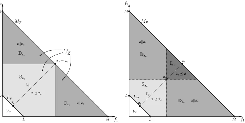
Figure 1. Trajectory for the experiment described in Section 3.4 comparing decomposition and Pareto-based methods. MPis the upper bound of
the feasible objective space while LPis the Pareto front and the lower bound of the feasible objective space. AlsoVFis the volume below the Pareto front andVZis the volume of the feasible objective space, whileVPis the volume of the region containing superior solutions to the current
solution zc. Lastly, zsand zeare the starting and target objective vectors, with zebeing Pareto optimal. The left figure illustrates the aforementioned quantities for zc=zsand the right figure illustrates how the above quantities change as zcmoves towards zealong the (ze−zs) direction. The results can be seen in Fig. (2).
the objective space, Z, is bounded from above by a hyperplane as shown in Fig. (1), specifically the upper bound is the set of points MP = {z : Pki=1zi = M,zi ≥0}. The reasons for selecting a feasible objective region with this
particular geometry will become clear in what follows. Also, let the Pareto front be a (k−1)-simplex, namely Pareto optimal objective vectors are part of the set LP ={z :Pki=1zi =L,zi ≥0}, obviously we have to select L < M for
minimization problems as L> M would imply Z ={∅}. If we also assume that the problem has no bias, then for a given objective vector, zc ∈Z, it would be possible to calculate the probability of obtaining a better solution for any
point in the objective space. This information can be useful in many ways, we elaborate on those in Section 6. Now, given a point in objective space, zcwhere the subscript is an abbreviation for current point, we can calculate
the probability of obtaining a better solution using the following relation,
P(z∈S|zc)= VS(zc)
VZ
, (3)
where,VS(zc)=VP(zc), for Pareto-based methods,VZis the volume of the feasible objective space which is equal
to the volume of the slab in between MP, LPand the positive orthantRk+, see Fig. (1). Additionally,P(z∈S|zc), is the
probability of finding a better objective vector, zn, given the objective vector zc. The expression in (3) is valid only for
problems whose objective function would produce objective vectors uniformly distributed, or nearly so, given a set of uniformly distributed decision vectors. For biased problems knowledge of the exact probability density function in objective space would be necessary so that we can weigh the integrals. However, as we mentioned above, in all but the most trivial problems the bias will be towards the Pareto front, otherwise it will be away from it, and so (3) will still describe a useful quantity, namely the upper bound of the probability of finding a better solution, assuming that there is no bias towards the Pareto front.
The volume of the region containing clearly better solutions,VP(zc), for Pareto dominance or cone dominance
using an ordering cone K=Rk +is,
VP(z)= k
Y
i=1
zi− VF, (4)
whereVF is the volume of the non-dominated region beneath the Pareto front, which is the volume beneath the
simplex, LP. The (k−1)-simplex corresponds to a Pareto front with affine geometry andVF is calculated as,
VL=
deth v1 · · · vk
i
Γ(k+1) . (5)
Here, vi, are the vertices that the Pareto front intersects with the axes andΓ(·) is the gamma function [2]. The vectors, vi for the Pareto front are equal to vi = L·ei, where ei is a vector of zeros and its ith element is equal to one.
Furthermore, the volume beneath the hyperplane MP,VM, is calculated using (5) and vi=M·ei. OnceVMandVL
have been evaluated, the volume of the entire feasible objective space is calculated as,
VZ=VM− VL. (6)
Also the volume of the non-dominated region forε-dominance is simply,
VPε(z)= k
Y
i=1
(zi−ε)− VF, (7)
assuming that the sameεvalue is used for every objective. If different values forεare used it is trivial to modify (7). The volume of the non-dominated region for coneε-dominance [4] is much more involved to calculate exactly, however, given that its defining set is the intersection of a proper cone and the setRk+εit stands to reason that its
volume,VKε, will be within,
VPε≤ VKε ≤ VP, (8)
depending on the selected acute cone.
3.4. Experiment
The question that we seek to answer is the following: Do decomposition-based optimization algorithms possess some inherent advantage over Pareto-based algorithms that can be attributed to the way partial ordering is induced in objective space? To answer this question we remove the implementation details of algorithms belonging to these families and study the effect of the fitness assignment on the likelihood that a superior solution is found as a function of the distance of the current best approximate solution to a solution on the Pareto front. To do this we select the shortest path in objective space from an initial point zsto a point on the Pareto front, ze, as shown in Fig. (1). Next we calculate
the probability of finding a better solution for points progressively closer to ze. This will inform us whether there is
some advantage in using decomposition-based methods over Pareto-based methods. However, there is an inherent assumption that approximate solutions in these algorithm families will tend to follow this particular trajectory. This means that we assume that if an algorithm starts from the point zs, intermediate solutions will tend to be close to the
trajectory shown in Fig. (1) and that upon convergence we will obtain the solution ze. Therefore we have to justify
two points, (i) why it would be reasonable to assume an algorithm would tend to follow this trajectory and (ii) why it should converge to that particular point, ze, and not any other point on the Pareto front. For decomposition-based
methods this is trivial as this is the direction in which the scalarization function monotonically decreases and the target point, ze, can be selected by appropriate selection of the weighting vector, w as shown in [12, 11]. And it is
conceivable that the point zeis part of a set of points that are targeted by the algorithm. For Pareto-based methods
however, even if we assume that a solution is admissible only when it dominates the current solution, zc, the end
point need not necessarily be ze. Nevertheless, this would be true only if we ignore the part of a Pareto-based method
that preserves diversity of solutions in objective space. Pareto-based algorithms as mentioned in the introduction will attempt to lead a set of solutions towards the Pareto front and simultaneously cover the entire Pareto front. This means that there is some mechanism to force solutions that are very close to each other in objective space to either move in unexplored regions of objective space or be eliminated. Indeed Pareto-based algorithms actively seek to preserve diversity and the employed measures are variations of the mean nearest neighbour distance in objective space [49]. This, in effect, allows an approximate solution to move only within a corridor in objective space. Given an adequate number of individuals in the EA this corridor can be approximated by a single trajectory as in Fig. (1) and the final solution will be withinεdistance from ze, whereεa small constant that can be made arbitrarily small by increasing
dist(ze,zc) P (z ∈ S | zc ) a) Pareto-Dominance
dist(ze,zc)
P (z ∈ S | zc )
b)ℓ1-norm
dist(ze,zc)
P (z ∈ S | zc )
c)ℓ2-norm
dist(ze,zc)
P (z ∈ S | zc )
d)ℓ∞-norm
0 2 4 6
0 2 4 6
0 2 4 6
0 2 4 6
10−30 10−25 10−20 10−15 10−10 10−5 100
10−30 10−25 10−20 10−15 10−10 10−5 100
10−30 10−25 10−20 10−15 10−10 10−5 100
[image:8.595.75.531.115.536.2]10−30 10−25 10−20 10−15 10−10 10−5 100
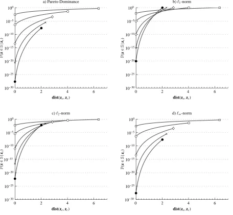
Figure 2. Probability of finding a better solution to zc,P(z∈S|zc), as a function of the Euclidean distance of the solution zcto ze, denoted by
dist(ze,zc), for different number of objectives (see Fig. (1)). Here{,◦,⋄,×,•}correspond to k={2,5,10,15,20}objectives respectively.
the trajectory in Fig. (1), then this will only serve to decrease the probability of finding a superior solution to the current point, as we have shown that algorithms whose solutions tend to wander in objective space tend, in the mean, to obtain inferior solutions [10]. Hence the obtained probabilities will still be an upper bound for the probability of finding a superior solution to the current solution, zc. This could be one reasons for the reported inferior performance
of Pareto-based algorithms.
Therefore, using (3)-(5) and a trajectory in objective space we can explore the change in the probability to obtain a solution inSfrom a current point, zc. Assuming we start from a point that is on the upper bound of the objective
space, zs ∈ MP, and a target point on the Pareto front ze, the question is how likely is to find a better solution with
respect to any point on the trajectory with direction ze−zs, see Fig. (1). This information for Pareto dominance
methods will give us a basis for comparison with other methods for inducing a partial order in the objective space and should illuminate any differences. The steps involved, for Pareto-based and decomposition-based methods described in Section 4, can be summarised as follows:
• Set zc=zs. Subsequently we divide the line segment from zsto zeinto N−1 segments, thus from start to end
there are N points zc[i]=zs+(ze−zs)Ni and i=0, . . . ,N−1, see Fig. (1).
• For every zc[i] we calculate (3). This procedure is illustrated in Fig. (1) and the results are shown in Fig. (2)-(a)
for Pareto-dominance methods.
[image:9.595.195.399.212.412.2]4. Decomposition Methods
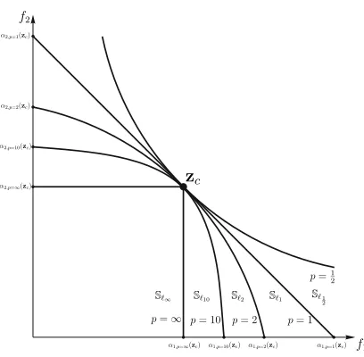
Figure 3. The curves in this figure represent the boundary of solutions that will be perceived as clearly better with respect to the corresponding p-norm.
4.1. Overview
An alternative for defining a partial order in objective space can be found in decomposition methods. As mentioned in Section 1, these methods employ a scalarizing function to aggregate all the objectives into a single scalar objective function. To obtain different Pareto optimal points, a set of weighting vectors can be used which would result in a set of single objective subproblems. This is the reason why such methods are called decomposition-based. It is because the employed strategy is to decompose a complex problem into a set of simpler ones. Simpler in this context does not necessarily mean easier to solve, it means that it is straightforward to apply standard EAs to the resulting subproblems. The family of scalarizing functions that we focus our attention in this work, is the weighted metrics method [34, pp. 97] defined as:
min
x
k
X
i=1
wi|fi(x)−z⋆i| p
1 p
, (9)
where, wiare the weighting coefficients, wi ≥0 for all i =1, . . . ,k, andPki=1wi =1, also p ∈ (0,∞). The vector z⋆ =(z
1, . . . ,zk), is called the ideal vector and is defined as z⋆ =(inf
x {f1(x)}, . . . ,infx {fk(x)}). For the purpose of this
work we will assume that z⋆=(0, . . . ,0), which means that (9) can be rewritten as,
min
x
k
X
i=1
wifi(x)p
1 p
. (10)
Notice that we are allowed to remove the absolute value while maintaining the equivalency relation between (9) and (10), since, z⋆ = (0, . . . ,0), implies that z ∈ Rk
+. The formulation shown in (10) obviates the relationship of the
weighted metrics scalarizing function with the weighting method and the Chebyshev decomposition. Namely, for
p=1 we obtain the weighting method [34, pp. 78],
min
x
k
X
i=1
wifi(x), (11)
while for p=∞we obtain the Chebyshev scalarizing function,
min
x (max{w1f1(x), . . . ,wkfk(x)}) . (12)
It should be noted that the assumption that the ideal vector is equal to the zero vector also implies that the objective function is bounded from below. In extension, if the ideal vector is known and is nonzero, a change of variables in the objective function would be sufficient to meet our assumption.
Although all norms are equivalent, in the sense that for every norm in a finite dimensional space multiplicative constants can be found relating two norms [6, pp. 636], their effect in an optimization problem can be significantly different, depending on the intricacies of the problem. For example, for p =∞, namely the Chebyshev scalarizing function, there exist theoretical results stating that the solutions of (12) will be at least weakly Pareto optimal for any weighting vector w∈Rk
+and that any Pareto optimal solution can obtained for some weighting vector [34, pp. 99].
The interest of the MOEA community with respect to this particular norm is that the previous statement holds for nonconvex problems as well. Note that this does not imply that there is a guarantee that the algorithm will be able to find a Pareto optimal solution for a nonconvex problem, rather the statement refers to the equivalency of the two problems. In other words, assuming that the selected algorithm is able to solve the problem defined in (12) then the solution will be at least a weakly Pareto optimal, and that all the Pareto optimal solutions can be obtained for some weighting vector. Such a result does not exist for p<∞. In Section 5 we show that, given some prior information, it is possible to find a norm other than infinity with the same properties mentioned above. Namely, the ability of the a scalarized problem to converge to a weakly Pareto optimal solution for every weighting vector w≻0 and that all
Pareto optimal solutions can be reached.
However, it is not obvious as to why a norm, other than theℓ∞-norm that is employed in the Chebyshev scalarizing
function, would be more useful for decomposing a multi-objective problem. For this reason we extend the experiment conducted for Pareto-based methods to decomposition-based methods that employ (10) as the scalarizing function to decompose a multi-objective problem and study the effects that different values of p have on the resulting subproblems, see Section 4.2.
4.2. Decomposition Methods for Multi-Objective Problems
The difference between scalarizing functions and the various forms of dominance relations discussed in Section 3, is that the former define a complete ordering in the objective space. Namely, regions containing incomparable solu-tions are eliminated, and depending on theℓp-norm used in (10), parts of theDregions are absorbed by the region
containing inferior solutions,I, and the region containing clearly better solutions,S. This phenomenon has the poten-tial to reduce the rate of decrease of the probability that a better solution is generated as the current solution approaches the optimal point, see Fig. (2)-(b-d). A better solution in this context is a solution that yields a lower value for the se-lected scalarizing function. In turn, this can reduce algorithm stagnation caused by a large number of non-dominated solutions, a phenomenon observed in Pareto-based methods [24]. Consider a scenario in which the weighted sum method is used. In this scenario the weighting vector represents the normal of a hyperplane that divides the feasible objective space in two partitions. One, a region containing better solutions,Sℓ1, and one with worse solutions,Iℓ1,
shown in Fig. (3). Solutions above the hyperplane are considered to be worse while solutions below the hyperplane are taken to be better with respect to the particular subproblem. Therefore, since the volume of theSregion is larger comparatively to dominance-based methods, it would be easier for the algorithm to identify solutions that are some-what closer to the front with respect to the currently best objective vector. However we have made a concession here, as the new solution may not Pareto-dominate the previous best solution. We will return to this issue in Section 5 and Section 6.
To explore how decomposition-based methods relate to Pareto-based methods, we must be able to calculate (3) for every p= (0,∞]. The volume of the feasible objective space is calculated in the same way as in (6), while the
volume of theSregion for p=(0,∞) is calculated as:
VSℓ
p(z)=
Γ1+1pk Γkp+1
· k
Y
i=1
αi(z)− VF, (13)
which is essentially the volume of the positive orthant of a hyperellipsoid calculated as seen in [45]. The factors ai(z)
represent the distance of the ideal vector from the intersection of the ellipsoid with the positive axis of the ithobjective,
shown in Fig. (3) and are calculated as,
αi(z)=
Pk
m=1wmz p m wi 1 p , (14)
see [45]. Since for the special case that p=∞,
lim
p→∞
Γ1+1pk Γkp+1
=1, (15)
the volume of theSregion becomes,
VSℓ∞(z)=α1(z). . . αk(z)− VF, (16)
and,
αi(z)=
max{w1z1, . . . ,wkzk}
wi
. (17)
Furthermore, to replicate the selected trajectory described in Section 3.3 and shown in Fig. (1), the weighting vector is set to w=1k·(1, . . . ,1) ascribing equal importance to all objectives so the resulting subproblem will tend to follow this trajectory and converge to the point ze. For this particular weighting vector (16) becomes,
max{w1z1, . . . ,wkzk}=wmzm,
VSℓ ∞(z)=
(1k)kzkm
(1k)k − VF =z k m− VF.
(18)
However, as can be seen in Fig. (1), all points in the trajectory from zsto zehave z1 =z2=· · ·=zk, hence zm=zifor
all i=1, . . . ,k, thus (18) can be calculated for any point on the trajectory.
As seen in Fig. (2)-(a-d), the probability of finding a better solution as zcapproaches the optimal solution ze
de-creases more rapidly for the Chebyshev scalarizing function and Pareto-based methods when compared to scalarizing functions employing theℓ1-,ℓ2-norm. However, the results for the Chebyshev scalarizing function are remarkably
similar to the Pareto-based method. In fact, for this trajectory, the two are identical, see (4) and (18). This interesting result means that Pareto-based methods and decomposition-based methods using the Chebyshev scalarizing function are identical in the sense that,
VSℓ
∞ =VP. (19)
This result is quite intriguing given the increased number of reports showing decomposition-based algorithms out-performing their Pareto-based counterparts for multi-objective problems [22, 23, 37, 20, 42]. However, we have only shown that the above equality holds for one particular trajectory and not necessarily for every possible trajectory towards any point on the Pareto front. We claim that (19) holds for an entire family of trajectories and that these particular trajectories are the ones that both decomposition and dominance-based algorithms attempt to follow in their approach towards the PF.
Consider a subproblem defined by the following weighting vector,
w=
c
1
s, . . . , ck s , s= k X i=1
ci,ci∈R+
(20)
and the trajectory defined by,
zc=C·
s c1
!1p
, . . . , s
ck
!1p
, s= k X i=1
ci,ci∈R+,C∈[L,M].
(21)
The starting point, zsis defined for C=M and the end point, ze(Pareto optimal point), for C=L. For this trajectory,
VP(zc)=
Y
i=1
kzc,i− VF =
(C s)k
Qk
i=1ci
− VF, (22)
and
VSℓ ∞(zc)=
(max{w1zc,1, . . . ,wkzc,k})k
Qk
i=1wi
− VF
= (C s)
k
Qk i=1ci
− VF.
(23)
At this point we need to justify the assumption that a solution will attempt to follow the trajectory (21) defined by a weighting vector (20), since it appears to be artificial. For this we refer to the work by Ballestero [3] where the author refers to this trajectory as well-balanced baskets due to the relation,
w1z1=w2z2=· · ·=wkzk, (24)
for a solution z ∈Z. This essentially describes the action of the scalarizing function on the objective vector, which
is to minimize the largest deviation in the givenℓp-norm. This is most easily observed in theℓ∞-norm used by the
Chebyshev decomposition whereby only the largest deviation is taken into account thus reeling the solution toward the balanced trajectory. By this reasoning, when theℓ∞-norm is used in a minimization problem, the focus of the
algorithm will be to maintain the Hadamard product w◦z as close as possible to the vector C·1 while attempting
to minimizekC·1k. By changing the weighting vector, this equilibrium that the Chebyshev scalarizing function is attempting to maintain, changes, so a different trajectory is followed, which of course converges to a different Pareto optimal point if the optimization algorithm is successful. That trajectory can be identified by finding the objective vector that sends the weighting vector w to the unit vector. This means that whenever the objective vectors are allowed to follow the balanced trajectory,VP(zc)=VSℓ
∞(zc).
It follows that for objective vectors following a balanced trajectory,
VSℓ1 >VSℓ2 >· · ·>VSℓ∞ =VP. (25)
Therefore, it follows that,
Pℓ1(z∈Sℓ1|zc)>Pℓ2(z∈Sℓ2|zc)> . . .
>Pℓ∞(z∈Sℓ∞|zc)=PP(z∈S|zc),
(26)
where z ∈ Z andSℓp is the region containing better solutions according to theℓp-norm version of the scalarizing
function andPℓp(z∈Sℓp) is the probability of finding a better solution inSℓpgiven that the current best solution is zc.
The result in (26) can be read directly from Fig. (3). It is noteworthy that in the case where a Pareto-based algorithm is unable to follow a ballanced trajectory, it follows that it is likely, in the mean, to have a slower convergence rate compared with a decomposition-based algorithm [10]. However, as the probabilities in (26) are upper bounds for the probability of obtaining a better solution from a current solution, zc, this equation still holds.
5. Scalarization and Stability of the Equivalent Problem
The results in the previous section must be interpreted with care since (26) does not imply in any way that by using a scalarizing function based on a norm with p<∞, all the Pareto optimal solutions will be reachable. However
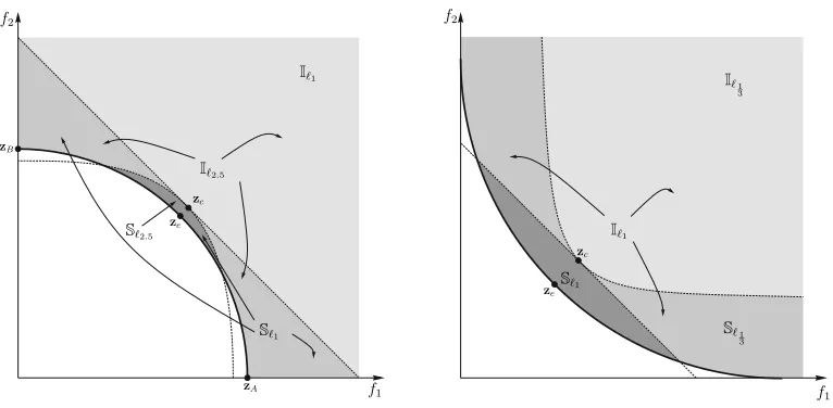
Figure 4. Stable and unstable scalarizing functions.VPF is the volume bounded by the ideal vector, z⋆, and the Pareto front.
it does imply that by using a scalarizing function with p small, there is a better chance in finding better solutions with respect to that norm. Nevertheless, we require Pareto optimal solutions and not just any solutions that are closer to the front in someℓp-norm, which means that if we cannot ensure that the subproblems are able to converge to Pareto
optimal solutions and that all Pareto optimal solutions will be obtainable, the importance of (26) would be limited to the fact that Pareto-dominance methods are equivalent to decomposition-based methods that employ the Chebyshev scalarizing function. Equivalent in the sense that for an objective vector following a well balanced trajectory the probability to obtain a solution dominating the current solution is the same in both methods.
To understand the tradeoffbetween using a dominance-based method versus a decomposition-based method let us consider the effect of a scalarizing function on the objective space. A scalarizing function projects the entire objective space onto a line5, therefore some regions that contain incomparable solutions in the Pareto sense, now
become solutions that are either better or worse for the particular subproblem. Therefore, a major difference between decomposition-based and Pareto-based algorithms is that the former provide unambiguous information about the quality of the produced solutions at every iteration while the latter cannot always guarantee such information because the likelihood of generating incomparable solutions is high for problems with a large number of objectives [24]. However it is easy to reduce the above argument into a deadlock between Pareto-based methods and decomposition-based methods. This is accomplished by the simple observation that the clearly better regions in the Chebyshev scalarizing function (p= ∞in Fig. (3)) are identical to the regions generated by Pareto dominance based methods, while the incomparable and clearly worse regions in Pareto-based methods are mapped to clearly worse regions by the Chebyshev scalarizing function. Namely, if we require a decomposition method that can guarantee the generation of Pareto optimal solutions, then, we have to use the Chebyshev scalarizing function, but in so doing we give up the favourable convergence rates6achieved when using, for example the weighted sum method, and vice versa. In general there are two competing trends:
• As p→0, the probability of finding a better solution with respect to theℓp-norm increases, hence it is less likely
that the algorithm stagnates due to its inability to find direction of search. Additionally, it becomes increasingly more difficult to obtain all Pareto optimal solutions.
• However, as p → ∞, we can obtain more Pareto optimal solutions on the Pareto front, but the probability of finding a better solution with respect to the norm defined by p is also decreasing. In the limit, namely for p=∞, we obtain the Chebyshev scalarizing function that guarantees that we will be able to find all Pareto
5In this work a segment of a ray, since the objective space is bounded. 6Or more correctly the potential for favourable convergence rates.
optimal solutions for some weighting vector w but this scalarizing function is equivalent with Pareto-dominance methods.
So the question is: is there a way that a scalarizing function can be used with p relatively small while preserving the guarantees that the Chebyshev function provides? The answer is affirmative for multi-objective problems whose Pareto front geometry is continuous (see Section 2) and can be described by the following parametrization,
fp1
1 +f
p2
2 +· · ·+ f pk
k =C, (27)
where pi > 0 for all i and C is a positive constant. This parametrization for the Pareto front is often used in the
literature, see for example [29, 28, 15]. For simplicity we assume that fi≥0. We claim that if the weighted metrics
scalarizing function is used with p =max{p1, . . . ,pk}, then this scalarization will have the same guarantees as the
Chebyshev function, given that our estimate of max{p1, . . . ,pk}is correct and that the objective function is continuous.
The reason for this is illustrated in Fig. (4). To see this, consider that when zcreaches zein Fig. (4), the volume of the
regionSℓ1is still positive, meaning that according to theℓ1-norm there are still better solutions to the current solution.
Continuing on the same line of reasoning, the solution zcwill either converge to zAor zBsince at these two locations
there is no way that theℓ1-norm to be improved. This result follows directly from (25) and the results in [45] for
calculating the volume in (27), it follows that,
lim
zc→ze
VPF − Vℓp
≤0, (28)
when p > max{pi}, in which case we say that the scalarization is stable while if p < max{pi}the scalarization is
unstable and we have,
lim
zc→ze
Vℓp− VPF
>0. (29)
where,VPF, is the volume of the region enclosed by the Pareto-front and the ideal vector z⋆as shown in Fig. (4).
Stability in terms of sclarizations is taken to mean the following:
• A subproblem of a multi-objective problem is a stable scalarization if for a given weighting vector w≻0, it is
able to converge to a Pareto optimal solution ze=(z1, . . . ,zk), with zi>0 for every i=1, . . . ,k.
• Conversely, a subproblem is an unstable scalarization if for a given weighting vector w≻0, it converges to a
Pareto optimal solution zewith zi=0 for at least one i∈ {1, . . . ,k}.
Therefore, if the Pareto front geometry is known and it can be expressed in terms of (27), then we can select the
ℓp-norm that will have the maximum probability to produce better solutions while preserving the guarantee that the
final population will be (weakly) Pareto optimal and that all the Pareto optimal solutions will be obtainable for some weighting vector.
6. Discussion
By calculating the probability to find a better solution, we have essentially turned the problem of extending a multi-objective optimization algorithm into a functional optimization problem. Namely, the question that can now be posed is: “what is the optimalℓp-norm for the scalarization and trajectory for an objective vector?”. By optimal
trajectory we mean the trajectory in objective space that will present the least resistance to our optimization algorithm while simultaneously moving towards a Pareto optimal solutions as fast as possible. This question, although very interesting, it either has a trivial answer: the straight line connecting the current solution zcto the target solution, or
for biased problems knowledge of the probability density function in the objective space is required, something which, in general, is unknown even for test problems. Therefore, we use a balanced trajectory, since this is in accord with the scalarizing functions, in the sense that this is the path that they tend to follow. Using this we investigated how the probability to obtain better solutions varies as a function of the distance of the current best solution and the sought for Pareto optimal solution. We found that this probability is largest the smaller theℓp-norm is, with respect to p. This
However, we cannot simply use the smallest norm that is numerically feasible since with decreasing p the ability of a scalarizing function to converge to a particular point of the Pareto front is also reduced, hence, a concession must be made. Although, if the Pareto front is continuous and can be described in a parametric way (see (27)), an optimal value, p⋆, can be obtained for which the decrease of the probability of finding a better solution is minimal while
the ability of the scalarizing function of finding every Pareto optimal solution is retained. The optimal value of p, separates the family of scalarizing functions into two subclasses. First, values of p<p⋆produce unstable scalarizing
functions and p > p⋆ result in stable scalarizing functions. Here stability refers to the ability of the scalarizing
function to converge to any point on the Pareto front, while instability refers to the opposite.
7. Conclusion
Based on the results in Section 3 and Section 4 we have seen that under mild conditions the Chebyshev function is identical to Pareto-dominance methods. Identical in the sense that, for a solution following a balanced trajectory, the reduction of probability to find a better solution is identical for both methods. This curious fact suggests that the decomposition-based methods using the Chebyshev scalarizing function are actually not better compared with Pareto-based methods. But if that is so, how can the results observed by several researchers for multi-objective problems be justified? Given the fact that the reported results are only slightly better in [16, 20] our hypothesis is that the difference is simply due to the ease with which a constant direction of search in objective space can be maintained in decomposition-based methods, while the same is very difficult to achieve with Pareto-based methods. This argument is further supported by the results in [10], where we show that varying weighting vectors can have significant impact on algorithm convergence. A good example of this behaviour is seen in a variation of MOGLS7 [27], initially introduced by [21, 25], when compared with MOEA/D in [47]. In the aforementioned work MOGLS was outperformed by MOEA/D, and as the authors note, one reason was that MOGLS generated different weighting vectors on every iteration. This amounts to an attempt to identify the entire Pareto front, but also means that the direction of search in objective space is not constant as is the case for MOEA/D. The same problem is present in Pareto-based methods, however there is no clear way for this situation to be remedied. Another potential cause for the apparent disparity in performance between Pareto-based methods and Decomposition-based methods is that the aforementioned equivalence depends on the degree to which Pareto-based methods are able to follow a balanced trajectory, and, in higher dimensions this would potentially be more challenging due to the relative lower density of solutions.
The results in this work show that:
• Pareto-dominance methods and the Chebyshev scalarizing function are equivalent, in the sense that neither method in itself, has better probability to find superior solutions. In fact the aforementioned probabilities are the same.
• Given some prior information about the problem, namely the geometry of the Pareto front, we can find the
optimal scalarizing function. Optimal in this context means that using the above scalarizing function all Pareto
optimal solutions will be obtainable for some weighting vector, and that, the probability of obtaining a bet-ter solution, with respect to the particular scalarizing function, decreases more slowly compared to all other scalarizing functions (and Pareto-dominance methods) that can provide the same guarantee of finding all Pareto optimal solutions.
• Using generalized decomposition (gD) [11, 12] in conjunction with the results in this work, the required weight-ing vectors for obtainweight-ing Pareto optimal solutions in specific locations on the Pareto front, can be identified for anyℓp-norm.
Some of the mentioned benefits apply only when we are able to identify the Pareto front geometry prior to obtaining Pareto optimal solutions.
7Multi-Objective Genetic Local Search.
References
[1] M. Ali, P. Siarry, M. Pant, An efficient differential evolution based algorithm for solving multi-objective optimization problems, European Journal of Operational Research 217 (2) (2012) 404–416.
[2] E. Artin, M. Butler, The gamma function, Holt, Rinehart and Winston New York, 1964.
[3] E. Ballestero, Selecting the CP Metric: A Risk Aversion Approach, European Journal of Operational Research 97 (3) (1997) 593 – 596. [4] L. Batista, F. Campelo, F. Guimar˜aes, J. Ram´ırez, Pareto Coneε-Dominance: Improving Convergence and Diversity in Multiobjective
Evolutionary Algorithms, in: Evolutionary Multi-Criterion Optimization, Springer, 2011, pp. 76–90.
[5] Y. Bengio, Y. LeCun, Scaling Learning Algorithms Towards AI, Large-Scale Kernel Machines 34 (2007) 1–41. [6] S. Boyd, L. Vandenberghe, Convex Optimization, Cambridge University Press, 2004.
[7] J. Chen, Q. Lin, Z. Ji, A hybrid immune multiobjective optimization algorithm, European Journal of Operational Research 204 (2) (2010) 294–302.
[8] R. C. Eberhart, J. Kennedy, A new optimizer using particle swarm theory, in: Proceedings of the sixth international symposium on micro machine and human science, vol. 1, New York, NY, 1995, pp. 39–43.
[9] P. Fleming, R. Purshouse, Evolutionary Algorithms in Control Systems Engineering: A Survey, Control Engineering Practice 10 (11) (2002) 1223–1241.
[10] I. Giagkiozis, R. Purshouse, P. Fleming, Towards understanding the cost of adaptation in decomposition-based optimization algorithms, in: IEEE International Conference on Systems, Man and Cybernetics, 2013, pp. 615–620.
[11] I. Giagkiozis, R. Purshouse, P. Fleming, Generalized decomposition and cross entropy methods for many-objective optimization, Information Sciences Available Online (2014) 1–25.
[12] I. Giagkiozis, R. C. Purshouse, P. J. Fleming, Generalized decomposition, in: Evolutionary Multi-Criterion Optimization, vol. 7811 of Lecture Notes in Computer Science, Springer Berlin Heidelberg, 2013, pp. 428–442.
[13] I. Giagkiozis, R. C. Purshouse, P. J. Fleming, An overview of population-based algorithms for multi-objective optimisation, International Journal of Systems Science Available Online (2013) 1–28.
[14] D. Goldberg, J. Holland, Genetic Algorithms and Machine Learning, Machine Learning 3 (2) (1988) 95–99.
[15] F. Gu, H. Liu, K. Tan, A Multiobjective Evolutionary Algorithm Using Dynamic Weight Method, International Journal of innovative Com-puting, Information and Control 8 (5B) (2012) 3677–3688.
[16] D. Hadka, P. Reed, Diagnostic assessment of search controls and failure modes in many-objective evolutionary optimization, Evolutionary Computation 20 (3) (2012) 423–452.
[17] J. Holland, Outline for a logical theory of adaptive systems, Journal of the ACM (JACM) 9 (3) (1962) 297–314.
[18] Q. Hu, A. Lim, An iterative three-component heuristic for the team orienteering problem with time windows, European Journal of Operational Research 232 (2) (2014) 276–286.
[19] S. Huband, P. Hingston, L. Barone, L. While, A Review of Multiobjective Test Problems and A Scalable Test Problem Toolkit, IEEE Transactions on Evolutionary Computation 10 (5) (2006) 477–506.
[20] H. Ishibuchi, N. Akedo, H. Ohyanagi, Y. Nojima, Behavior of emo algorithms on many-objective optimization problems with correlated objectives, in: IEEE Congress on Evolutionary Computation, 2011, pp. 1465 –1472.
[21] H. Ishibuchi, T. Murata, A multi-objective genetic local search algorithm and its application to flowshop scheduling, Systems, Man, and Cybernetics, Part C: Applications and Reviews, IEEE Transactions on 28 (3) (1998) 392–403.
[22] H. Ishibuchi, Y. Sakane, N. Tsukamoto, Y. Nojima, Effects of using two neighborhood structures on the performance of cellular evolutionary algorithms for many-objective optimization, in: IEEE Congress on Evolutionary Computation, 2009, pp. 2508 –2515.
[23] H. Ishibuchi, Y. Sakane, N. Tsukamoto, Y. Nojima, Evolutionary Many-Objective Optimization by NSGA-II and MOEA/D with Large
Populations, in: IEEE International Conference on Systems, Man and Cybernetics, 2009, pp. 1758 –1763.
[24] H. Ishibuchi, N. Tsukamoto, Y. Nojima, Evolutionary many-objective optimization: A short review, in: IEEE Congress on Evolutionary Computation, 2008, pp. 2419 –2426.
[25] H. Ishibuchi, T. Yoshida, T. Murata, Balance Between Genetic Search and Local Search in Memetic Algorithms for Multiobjective Permuta-tion Flowshop Scheduling, IEEE TransacPermuta-tions on EvoluPermuta-tionary ComputaPermuta-tion 7 (2) (2003) 204–223.
[26] S. Jakobs, On genetic algorithms for the packing of polygons, European Journal of Operational Research 88 (1) (1996) 165–181.
[27] A. Jaszkiewicz, On the Performance of Multiple-Objective Genetic Local Search on the 0/1 Knapsack Problem - A comparative Experiment, IEEE Transactions on Evolutionary Computation 6 (4) (2002) 402–412.
[28] S. Jiang, Z. Cai, J. Zhang, Y.-S. Ong, Multiobjective optimization by decomposition with pareto-adaptive weight vectors, in: International Conference on Natural Computation, vol. 3, 2011, pp. 1260 –1264.
[29] S. Jiang, J. Zhang, Y. Ong, Asymmetric pareto-adaptive scheme for multiobjective optimization, in: Advances in Artificial Intelligence, vol. 7106 of Lecture Notes in Computer Science, Springer Berlin Heidelberg, 2011, pp. 351–360.
[30] D. Karnopp, Random search techniques for optimization problems, Automatica 1 (2-3) (1963) 111–121.
[31] J. Kennedy, R. Eberhart, Particle Swarm Optimization, in: IEEE International Conference on Neural Networks, vol. 4, IEEE, 1995, pp. 1942–1948.
[32] H. Li, Q. Zhang, Multiobjective Optimization Problems with Complicated Pareto Sets, MOEA/D and NSGA-II, IEEE Transactions on
Evolutionary Computation 13 (2) (2009) 284–302.
[33] M. Luhandjula, M. Rangoaga, An approach for solving a fuzzy multiobjective programming problem, European Journal of Operational Research 232 (2) (2014) 249–255.
[34] K. Miettinen, Nonlinear Multiobjective Optimization, vol. 12, Springer, 1999.
[35] N. Radcliffe, P. Surry, Fundamental Limitations on Search Algorithms: Evolutionary Computing in Perspective, in: Computer Science Today, vol. 1000 of Lecture Notes in Computer Science, Springer Berlin/Heidelberg, 1995, pp. 275–291, 10.1007/BFb0015249.
[36] I. Rechenberg, Cybernetic solution path of an experimental problem, in: Royal Aircraft Establishment Translation No. 1122, Translated by B. F. Toms, Ministry of Aviation, Royal Aircraft Establishment, 1965.
[37] D. Saxena, Q. Zhang, J. Duro, A. Tiwari, Framework for many-objective test problems with both simple and complicated pareto-set shapes, in: Evolutionary Multi-Criterion Optimization, Springer, 2011, pp. 197–211.
[38] O. Schutze, A. Lara, C. Coello, On the Influence of the Number of Objectives on the Hardness of a Multiobjective Optimization Problem, IEEE Transactions on Evolutionary Computation 15 (4) (2011) 444 –455.
[39] F. J. Solis, R. J.-B. Wets, Minimization by random search techniques, Mathematics of operations research 6 (1) (1981) 19–30.
[40] R. Storn, K. Price, Differential evolution–a simple and efficient heuristic for global optimization over continuous spaces, Journal of global optimization 11 (4) (1997) 341–359.
[41] R. Takahashi, E. Carrano, E. Wanner, On a stochastic differential equation approach for multiobjective optimization up to pareto-criticality, in: Evolutionary Multi-Criterion Optimization, vol. 6576 of Lecture Notes in Computer Science, Springer Berlin, 2011, pp. 61–75. [42] Y.-Y. Tan, Y.-C. Jiao, H. Li, X.-K. Wang, MOEA/D+uniform design: A new version of MOEA/D for optimization problems with many
objectives, Computers & Operations Research 40 (6) (2013) 1648–1660.
[43] M. F. Tasgetiren, Y.-C. Liang, M. Sevkli, G. Gencyilmaz, A particle swarm optimization algorithm for makespan and total flowtime mini-mization in the permutation flowshop sequencing problem, European Journal of Operational Research 177 (3) (2007) 1930–1947.
[44] C. Vira, Y. Haimes, Multiobjective Decision Making: Theory and Methodology, No. 8, North-Holland, 1983. [45] X. Wang, Volumes of Generalized Unit Balls, Mathematics Magazine 78 (5) (2005) 390–395.
[46] D. Wolpert, W. Macready, No Free Lunch Theorems for Optimization, IEEE Transactions on Evolutionary Computation 1 (1) (1997) 67–82. [47] Q. Zhang, H. Li, MOEA/D: A Multiobjective Evolutionary Algorithm Based on Decomposition, IEEE Transactions on Evolutionary
Com-putation 11 (6) (2007) 712–731.
[48] E. Zitzler, K. Deb, L. Thiele, Comparison of Multiobjective Evolutionary Algorithms: Empirical Results, Evolutionary Computation 8 (2) (2000) 173–195.
[49] E. Zitzler, L. Thiele, An evolutionary algorithm for multiobjective optimization: The strength pareto approach, Swiss Federal Institute of Technology, TIK-Report 43 (1998) 1–43.
[50] E. Zitzler, L. Thiele, Multiobjective Evolutionary Algorithms: A Comparative Case Study and the Strength Pareto Approach, IEEE Transac-tions on Evolutionary Computation 3 (4) (1999) 257–271.