A new approach to the method of source-sink potentials for molecular conduction

Barry T. Pickup, Patrick W. Fowler, Martha Borg, and Irene Sciriha

Citation: The Journal of Chemical Physics 143, 194105 (2015); doi: 10.1063/1.4935716 View online: http://dx.doi.org/10.1063/1.4935716

View Table of Contents: http://scitation.aip.org/content/aip/journal/jcp/143/19?ver=pdfcov Published by the AIP Publishing

Articles you may be interested in

Extension of the source-sink potential (SSP) approach to multichannel quantum transport J. Chem. Phys. 137, 174112 (2012); 10.1063/1.4764291

Two-channel conduction through polyacenes—Extension of the source–sink potential method to multichannel coupling to leads

J. Chem. Phys. 134, 044119 (2011); 10.1063/1.3535117

Conduction in graphenes

J. Chem. Phys. 131, 244110 (2009); 10.1063/1.3272669

Group theory approach to the Dirac equation with a Coulomb plus scalar potential in D+1 dimensions J. Math. Phys. 44, 4467 (2003); 10.1063/1.1604185

Analytical investigations of an electron–water molecule pseudopotential. II. Development of a new pair potential and molecular dynamics simulations

J. Chem. Phys. 117, 6186 (2002); 10.1063/1.1503308

A new approach to the method of source-sink potentials

for molecular conduction

Barry T. Pickup,1,a)_{Patrick W. Fowler,}1,a)_{Martha Borg,}1_{and Irene Sciriha}2 1_{Department of Chemistry, University of Sheffield, Sheffield S3 7HF, United Kingdom} 2_{Department of Mathematics, University of Malta, Msida, Malta}

(Received 12 August 2015; accepted 3 November 2015; published online 19 November 2015)

We re-derive the tight-binding source-sink potential (SSP) equations for ballistic conduction through conjugated molecular structures in a form that avoids singularities. This enables derivation of new results for families of molecular devices in terms of eigenvectors and eigenvalues of the adjacency ma-trix of the molecular graph. In particular, we define the transmission of electrons through individual molecular orbitals (MO) and through MO shells. We make explicit the behaviour of the total current and individual MO and shell currents at molecular eigenvalues. A rich variety of behaviour is found. A SSP device has specific insulation or conduction at an eigenvalue of the molecular graph (a root of the characteristic polynomial) according to the multiplicities of that value in the spectra of four defined device polynomials. Conduction near eigenvalues is dominated by the transmission curves of nearby shells. A shell may be inert or active. An inert shell does not conduct at any energy, not even at its own eigenvalue. Conduction may occur at the eigenvalue of an inert shell, but is then carried entirely by other shells. If a shell is active, it carries all conduction at its own eigenvalue. For bipartite molecular graphs (alternant molecules), orbital conduction properties are governed by a pairing the-orem. Inertness of shells for families such as chains and rings is predicted by selection rules based on node counting and degeneracy. C _{2015 AIP Publishing LLC.[http:}//_dx.doi.org/_10.1063/_1.4935716]

I. INTRODUCTION

The subject of unimolecular electrical conduction and devices based on it has a venerable history,1–5and has a vast research literature; a recent review article has an impressive 607 references,6 and reviews,7,8 journal special issues and discussion volumes9–11and books12,13devoted to the different aspects of the topic continue to appear.

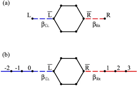
The present paper deals with an attractive approach for qualitative modelling of single-molecule conduction, due to Ernzerhof and his group. The Source-Sink Potential (SSP) model14–27 _{is a simple and convenient methodology for the} study of ballistic electronic conduction through molecular devices. The method uses a model device depicted in Fig.1(a)

in which a molecule is attached to a source atom, L, that creates a flux of electrons, and to a sink atom, R, that destroys it. The electron flux through the model device is designed to be identical to that in a cognate device (the lower diagram of Fig. 1) with infinite wires, in which an electron beam with wavevector qL in the left wire is partly transmitted through the molecule, emerging as a beam of wavevector qR

in the right. In this work, we consider an n-atom molecular π-system based on a carbon skeleton and treat it using the Hückel (tight-binding) formalism. The molecular adjacency matrix is A, where Apq=1 if p_,q and p is bonded to q, and Apq=0 otherwise. The connections L ¯L and ¯RR have resonance parametersβLL¯ andβRR¯ , respectively. The molecule

has resonance parameter β, and coulomb parameterα. In the usual system of units,αis set to zero, and_|β_|is taken as 1.

a)_{Authors to whom correspondence should be addressed. Electronic}

addresses: [email protected] and [email protected]

We have previously utilised the SSP formalism to derive analytical expressions for electronic transmission.28–35_{In our} approach, the solutions for an incoming beam of electrons with energyEare written in terms of five molecularstructural poly-nomials, which comprise the real characteristic polypoly-nomials,28

s=det(E1−A),

t=det₍E1−A_)[L¯,L¯], u=det(E1−A)[R¯,R¯], v =det₍E1−A_)[L ¯¯R,L ¯¯R],

=(−1)L¯+R¯_det

(E1−A)[L¯,R¯],

(1)

where the superscripts in braces indicate which rows (left) and columns (right) corresponding to connection atoms ¯L and/or

¯

R are to be struck out from the characteristic matrices. The polynomial, , with row ¯L and column ¯R removed from the determinant satisfies the Jacobi-Sylvester relation36

2_{=ut−sv. (2)}

The expression for the overall transmission28is

T(E)=B₍qL,qR)  2

|D_|2, (3)

whereEis the energy of the incoming stream of electrons and

B₍qL,qR)=(2βLsinqL)(2βRsinqR)β2_LL¯ β 2 ¯

RR (4)

and

D₍E₎=βLe−iqLβRe−iqRs−βRe−iqRβLL2¯ t

−βLe−iqLβ2

¯ RRu+β

2 ¯ LLβ

2 ¯

RRv. (5)

0021-9606/2015/143(19)/194105/20/$30.00 143, 194105-1 © 2015 AIP Publishing LLC

FIG. 1. (a) A SSP molecular device comprising a molecule attached to source and sink atoms L and R via contacts ¯L and ¯R, respectively. (b) A molecule attached to infinite left- and right-hand wires, showing the numbering scheme adopted for the atoms in the wires.

Wavevectors qL and qR are functions of E and satisfy the dispersion relations

E=αL+2βLcosqL=αR+2βRcosqR. (6)

These dispersion relations are appropriate for the infinite wires in Fig.1(b), assuming Hückel parameters(αL, βL)and (αR, βR), for left and right wires, respectively.

The purpose of the current article is to present a reformulation of the SSP approach in Section III and then to use it to give simple derivations of a number of new results. We first set out the SSP secular equations in the standard atomic-orbital (AO) basis (Subsection III B), and then in the molecular-orbital (MO) basis (Subsection III C). We show that ballistic molecular conduction can be described in complementary ways: as transmission along bonds (graph edges) or through parallel channels based on molecular orbitals. In the latter description, molecular orbitals can be

inert, having no conduction at any energy (including the orbital eigenvalue), or they can beactive, and these properties obey selection rules based on degeneracy and nodal character. SectionsIV–VIIIdescribe the theoretical framework and give expressions from which orbital transmission can be calculated, and inert/active status decided.

The main new results obtained from the reformulation of the SSP equations are as follows. First, the reformulation itself removes singularities, giving confidence that the results are mathematically well defined at all energies. Second, SSP leads to a direct partition of total transmission into a sum of well-defined orbital contributions, avoiding the need for a post hoc projection scheme. Third, the analysis naturally establishes the dichotomy between inert and active orbitals and leads to selection rules to predict the character of a given orbital. Finally, as we discuss briefly in Sec. X, this opens up the way to improved treatment of the role of electron interaction in what is so far a purely Hückel-based model.

Readers interested only in the main chemical conclusions could consider skipping directly to SectionIXwhere illustra-tive examples are given, along with simple analytical formulas for devices based on paths (linear polyenes) and cycles (an-nulenes). An extended Sec. Xthen discusses the qualitative significance of the results derived in the main body of the paper.

II. TECHNICAL NOTES

The algebraic computations reported in this paper were all performed by using Maple 18.37 Computations for the figures were carried out using unbiased (αL=αR=0), and

symmetric devices (βL= βR), with specific valuesβL=1.4β

andβLL¯ = βRR¯ = β.

The equal βapproximation used in this paper is ideally adapted to small all-carbon frameworks, but the formalism we develop in terms of structural polynomials exhibited in Eqs.(1)and(3)applies equally to systems for which weighted graphs are appropriate. These include systems displaying π-distortivity,38,39 _{or doped with hetero-atoms which are, of} course, important in realistic applications.

Likewise, it may be noted that all applications of the SSP model in the present paper are based on devices with one-dimensional leads attached to single atoms of the molecule. More complicated leads and connection patterns can be accommodated by modification of the contents of the blocks of the device matrix (see Eqs.(25)and(32), later). Examples of SSP treatments of multichannel devices are given in Refs.27

and40.

The approach used here is grounded in qualitative molecular-orbital theory; this is a choice based on the belief that such models allow “for a transparent interpretation of molecular conductance in terms of discrete eigenstates.”19_The use, either explicit or implicit, of orbitals and orbital densities gives an opportunity for using familiar chemical concepts to give insight.22,26,41,42 _{Many researchers in the field use} Green’s Function approaches, particularly for calculation, and of course these too have their specific advantages. However, it has been shown that the two approaches, when used with the SSP model approximations, lead to identical expressions for transmission.33

A remark about notation: we will use labels p,q, . . .for atoms, k, k′, . . .for molecular orbitals, and K for shells.

III. A REDERIVATION OF THE SSP EQUATIONS

We begin by considering the normalisation of the wavefunctions for the full device that is replicated by the SSP device of Fig.1(a), and consists of the molecule with two attached infinite wires (cf. Fig.1(b)). The numbering scheme for atoms in Fig.1(b)is designed to simplify the algebra that follows by elimination of the unnecessary phase factors that have plagued previous derivations.18,26,28We first consider the normalisation of the wavefunctions for the infinite wires.

A. Flux normalization

The wavefunctions ψleft,ψright in left- and right-hand wires, respectively, are written in the tight-binding (Hückel) approximation as

ψleft ₌ 0 

p₌−∞

c_pleftφp,

ψright ₌

∞



p=1 crightp φp,

(7)

where theφpare basis functions on the atoms of left and right

wires, and the Hückel Coulomb and resonance parameters are αL, βL, andαR, βR, respectively. Coefficients for the left and

right wires are given by

c_pleft = 1 NL e

iqLp+_{r e}−iqLp_,

cpright =

1

NR

τeiqRp

(8)

for the specified boundary conditions, where the left-hand wavefunction is a combination of a forward-travelling wave

(eiqL_{) and a backward- travelling component(e}−iqL_{) with a} reflection coefficient,r. The molecule acts as a potential barrier that produces a reflected wave in the left wire and a forward transmitted wave₍eiqR_{)in the right wire, with a transmission} coefficient, τ. This corresponds to a flux of electrons with energyE, satisfying both Eq.(6)and the Hückel Schrödinger equation for infinite wires.

The total electron transmission probability is then

T₍E₎=1−_|r_|2=_|τ_|2. (9)

The normalisation factors NL and NR have been introduced to obtain the requisite unit electron flux. Hence, the current density43from atom(p−1)to atom p in the left wire, using the standard Hückel formulation, is

J₍left_p−1)→p=1 i

(

φp−1|Hˆ|φp

cleft_p−1∗cleftp −c.c. )

=2βLsinqL N2

L

1−_|r|2

, (10)

where we have used _⟨φp−1|Hˆ|φp⟩=βL. This expression is

independent of the index p, showing that a constant current flows down the wire. We require this current to be equal to the transmission probability,T₍E₎. Hence, we deduce that the correct flux normalisation is achieved by setting

N_L2=2βLsinqL (11)

and using an analogous derivation for the right-hand wire

N_R2=2βRsinqR. (12)

B. The SSP equations in the atomic orbital basis

The secular equations of the device shown in Fig.1(b)for atom 0 in the left-hand wire and for atom 1 in the right-hand wire are

βLc−left1 +(αL−E)cleft0 +βLL¯ c¯L = 0,

βRR¯ c¯R+(αR−E)c right 1 +βRc

right

2 = 0

(13)

where β_LL¯ , β_RR¯ are resonance parameters for the connections

from the wires to the molecule. We wish to replace the left wire by a single source atom, L, sited at atom 0 and creating a flux of electrons corresponding to the wavefunction ψleft in Eqs. (7) and (8). Similarly, we wish to replace the right wire by a single sink atom, R sited at atom 1 and removing the transmitted flux. This requires the definition of complex

potentials,ΘL,ΘR, on these source and sink atoms to replace

the effects of atoms to the left of atom 0, and to the right of atom 1, respectively.

Hence, we define

βLc−left1 = ΘLc0left,

βRcright₂ = ΘRcright₁ . (14)

The potentials can now be derived by using the expressions from Eq.(8)for the orbital coefficients

ΘL=βL

cleft₋₁

cleft 0

= βL

e−iqL+_{r e}iqL

(1+r₎ ,

ΘR= βR

c₂right

c₁right=

βReiqR.

(15)

In the standard SSP formalism,14,26,28 _{these potentials are} used directly in the SSP secular equations. However, when the reflection coefficient,r, becomes equal to−1, the potential

ΘLbecomes infinite. A more satisfactory approach, avoiding

this singularity, is obtained by substituting the explicit form ofcleft

−1 into Eq.(13)to give

βL NL

e−iqL+_{r e}iqL

+(αL−E)cL+β_LL¯ c¯_L=0 (16)

and noting from Eq.(8)that

cL≡c₀left=1+r

NL (17)

we deduce that

r=NLcL−1. (18)

Substituting forrin Eq.(16), we obtain

βLeiqL+α

L−E

cL+β_LL¯ c¯_L=

2iβLsinqL NL

=i NL, (19)

where we have placed the inhomogeneity on the right-hand side. We can carry out the same procedure usingcright₁ from Eq.(8)in Eq.(13)to give

cR≡c₁right= τ NR

eiqR ₍₂₀₎

and hence

c₂right=e2iqR τ

NR =e iq_R

cR. (21)

Substitution of this expression into Eq.(13)gives

βRR¯ c¯R+ αR−E+βReiqR

cR=0 (22)

which does not contain an inhomogeneity.

With these modifications to the boundary conditions, we can now find the wavefunction for the model device. The wavefunction

ψSSP= n



p=1

cpAOφp+cLφL+cRφR (23)

is the solution to the SSP equations in the AO formalism. The φp here are basis functions on the atomic centres, and

φL, φR are basis functions on source and sink atoms. The (n+2₎-dimensional SSP equations for the SSP device

depicted in Fig. 1(a) can now be written in matrix form as

PAO

* . . .

,

cAO

cL

cR

+ / / /

-=* . . .

,

0

−i NL

0 + / / /

-, (24)

where thedevice matrixis

PAO=

* . . .

,

E1−A −bL −bR

−b_L E−α_L−β_LeiqL 0 −bR 0 E−αR−βReiqR

+ / / /

-(25)

and where for our single-atom-contact configurations the

connectionmatrix elements are

(bL)p = δp ¯LβLL¯ , (bR)p = δp ¯RβRR¯

(26)

and the source and sink matrix elements are

E−αL−βLeiqL = βLe−iqL,

E−α_R−βReiqR = β_Re−iqR. (27)

Here, we have used dispersion relations Eq.(6)to removeE

from source and sink matrix elements.

The form of Eq. (24) conforms more closely than the previous formulation28 _{to the widely used Green’s function} approach,3 _{in that the electron flux arises from a single} inhomogeneity in the source L-element of the vector on the right-hand side of the equation.

C. The SSP equations in the MO basis

This section describes the form of the SSP matrix equations in the MO representation. This alternative form is useful for analysing the behaviour of the solution at the eigenvalues of the isolated molecule. The Hückel MOs

ψk= n



p=1

φpUpk (28)

diagonalize the secular matrix of the molecule, i.e.,

n



q₌1

ApqUqk=Upkϵkfor p=1,2, . . . ,n. (29)

We shall assume throughout this paper that since the

n×n-dimensional adjacency matrixAis real and symmetric, the matrix U can be considered to be orthogonal. Hence, we can define an augmented ₍n+2₎×₍n+2₎-dimensional orthogonal matrix

* . . .

,

U 0 0

0 1 0

0 0 1

+ / / /

-(30)

which can be used to transform AO-based SSP secular equations(13)to give the MO-based version

PMO

* . . .

,

cMO

cL

cR

+ / / /

-=* . . .

,

0

−i NL

0 + / / /

-, (31)

where the SSP device matrix in the MO basis is

PMO=

* . . .

,

p −uL −uR

−_uL βLe−iqL 0

−_uR 0 βRe−iqR

+ / / /

-(32)

and the diagonal MO-MO block has

pkk′=δ_kk′pk=δ_kk′=(E−ϵ_k). (33)

The connection matrix in the MO basis is more complicated than in the AO form, i.e.,

(uL)k= (



UbL )

k=βLL¯ U¯Lk, (uR)k=

(



UbR )

k=βRR¯ U¯Rk

(34)

and the MO expansion coefficients are related to those in the AO basis by

cMO=Uc AO. (35)

The SSP wavefunction, the solution to Eq.(31), is

ψSSP= n



k=1

c_kMOψk+cLφL+cRφR, (36)

where now theψkare MOs of the molecule, the coefficients cL,cRare identical in Eqs.(23)and(36), and the MO and AO coefficients are related as in Eq.(35).

The two expansions of the wavefunction ψSSP, i.e.,

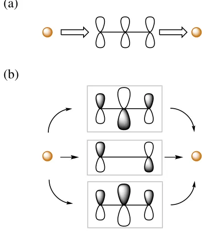
Eqs. (23) and (36), correspond to different models of the conduction process, as illustrated in Fig. 2 for the example of an end-to-end connected allyl chain. In one, the electron hops from AO to AO along edges of the molecular graph; in the other, the MOs act as parallel channels for conduction of electrons.

FIG. 2. Alternative schematic representations of ballistic conduction in a source-sink model device: (a) in the AO basis, where conduction between source and sink takes place via bonds between atoms carrying single basis functions, (b) in the MO basis, where the molecular orbitals act as parallel conducting channels between source and sink.

We note that all coefficientscL, cR,cMO_{, and c}AO_{are in}

general complex, but the transformation matrix Urefers to the unperturbed molecule and can always be chosen to be real. It may sometimes be convenient to use complex Ufor degenerate eigenvalues, but it is never necessary.

IV. A MATHEMATICAL TOOLKIT

The derivation of the solutions of the SSP equations and their analysis requires a mathematical investigation of the structural polynomials, and quantities related to them. We gather all this information together in the present section in order not to interrupt the flow of the rest of the derivation.

A. Structural polynomials in the MO basis

Our first aim is to express the structural polynomials in terms of the eigenvectors and eigenvalues of the adjacency matrix defined in Eq.(29). Hence,

s(E)=det(E1−A)= k

pk, (37)

where we have used the notation of Eq.(33), and the product runs over the whole molecular spectrum. We shall consider the general structural polynomials

rs = (−1)r+sdet(E1−A)[r,s],

vpqrs = (−1)p+q+r+sdet(E1−A)[pq,rs]

(38)

which include all the definitions in Eq.(1), viz.,

t=L ¯¯L,u=R ¯¯R, = L ¯¯R, v =vL ¯¯R ¯L ¯R. (39)

It can be shown that44

svpqrs={prqs}, (40)

which has been defined using the notation for the anti-symmetrised product

{XprXqs_}=XprXqs−XpsXqr. (41)

Eq.(40)is a more general form of the Jacobi-Sylvester relation given in Eq.(2).

It is also convenient to define a notation in which a “hat” symbol indicates a quantity divided by the polynomials,

ˆ

X = X

s. (42)

We shall refer to quantities such as ˆrsas “reduced” structural

polynomials. They can be shown to be matrix elements of the inverse of the characteristic matrix by using the well-known Cramer’s rule result

ˆ

rs=(−1)r+s

det₍E1−A₎[r,s]

det₍E1−A₎ =(E1−A)

−1

rs . (43)

The spectral representation follows directly as

ˆ rs=



k UrkUsk

E−ϵ_k. (44)

Defining the quantities

sk= s pk, skk′= s pkpk′

, (45)

we see that all the (real) characteristic polynomials of the device, Eq.(1), can be expressed in terms of these factors as

rs(E)= 

k

UrkUsksk,

vpqrs(E)= 

k>k′

{UpkUqk′}{UrkUsk′}skk′, (46)

where we have used Eqs.(40)and(43)to deduce the formula forv.

B. Expansion of the reduced structural polynomials

We shall need to expand the solutions of the SSP equations as a series around molecular eigenvalues. We also need to take into account the degeneracy,g, of such eigenvalues. We shall refer to a degenerate space as a “shell,” and use capital roman indices to label such shells. The individual MOs in the shell space, K, will then beψkfor k∈K. (Strictly,gisgK, but the K

dependence will be suppressed when there is no ambiguity.) To understand more fully what happens when the electron energy is at a shell eigenvalue,ϵK, we need to explore the behaviour

of the reduced structural polynomials near that eigenvalue. For the most general reduced structural polynomial shown in Eq.(38), we have

ˆ rs(E)=



k∈K UrkUsk E−ϵK+



a<K UraUsa E−ϵa

=

k UrkUsk

pK + 

a

UraUsa

ϵK−ϵa+pK

. (47)

In this equation, and in what follows, we use a convention in which the summation indices k,k′_{, . . ., label MOs inside} the degenerate shell K, and indices a,b, . . ., label MOs that are “off-shell,” without explicitly indicating the summation ranges. Within the radius of convergence, each reduced structural polynomial can be expanded in a Laurent series around the pointE=ϵK. We usepK=E−ϵKas the expansion

parameter. It is easy to deduce that

ˆ rs(E)=

ˆ rs,−1

pK +ˆrs,0+ˆrs,1pK+O(p 2

K), (48)

wherealldependence uponE is through powers of pK, and

the expansion coefficients are

ˆ rs,−1=



k

UrkUsk,

ˆ rs,0=



a

UraUsa (ϵK−ϵa)

,

ˆ rs,1=−



a

UraUsa (ϵK−ϵa)2

.

(49)

A similar derivation, using Eq.(40)in the form ˆvpqrs={ˆprˆqs},

produces

ˆ

vpqrs(E)=p−K2vˆpqrs,−2+pK−1vˆpqrs,−1

+vˆpqrs,0+vˆpqrs,1pK+O(p2K), (50)

where

ˆ v_pqrs,−2 =



k>k′

{UpkUqk′}{UrkUsk′},

ˆ v_pqrs,−1 =



k,a

{UpkUqa}{UrkUsa} (ϵK−ϵa)

,

ˆ v_pqrs,0 =



a>b

{UpaUqb}{UraUsb} (ϵK−ϵa)(ϵK−ϵb)

−

k,a

{UpkUqa_}{UrkUsa_} (ϵK−ϵa)2

.

(51)

The terms ˆrs,−1(and hence ˆt−1,uˆ−1, and ˆ−1) and ˆvpqrs,−2,vˆpqrs,−1

(and hence ˆv−2,vˆ−1), are all traces over the degenerate shell.

It is important to recognise that these are thereforeinvariant

to unitary transformations amongst the MOswithinthe shell subspace.

In later parts of this paper, we will need definitions of structural polynomials dependent only upon “off-shell” orbitals, i.e.,

sA(E)= a

pa,

ˆ

A,rs(E)= 

a UraUsa E−ϵa

,

ˆ

vpqrs,A(E)= 

a>b

{UpaUqb}{UraUsb} (E−ϵa)(E−ϵb)

,

(52)

where “A” denotes all eigenvectors associated with eigen-values ϵa,ϵK. These definitions are exactly analogous to

those in SectionIV A. It can be seen from Eqs.(47)and(48)

and(50)and(51), that the whole energy-dependence of the structural polynomials can be expressed as

pKˆrs(E)= ˆrs,−1+pKˆA,rs(E),

p_K2vˆpqrs(E)=vˆpqrs,−2+pKvˆpqrs,−1+ p2KvˆA,pqrs(E).

(53)

In our earlier papers,31,35 _{we have linked conduction and} insulation properties to the interlacing properties of the eigenvalues of a graph. Since

s(E)=p_KgsA(E), (54)

we deduce that the polynomials can be writtenexactlyin terms of the degeneracy as

rs(E)=pg

−1 K sA(E)

ˆ

rs,−1+pKˆA,rs(E)

_,

ˆ

vpqrs(E)=p

g−2 K sA(E)

ˆ

vpqrs,−2+pKvˆpqrs,−1 + p2_KvˆA,pqrs(E)

_.

(55)

The Laurent expansion about the shell eigenvalue equivalent to these expressions is

rs(E)=pg_K−1sA(E) (ˆrs,−1+ˆrs,0pK + ˆrs,1pK2+· · ·

_,

ˆ

vpqrs(E)=p

g−2

K sA(E) vˆpqrs,−2+vˆpqrs,−1pK + vˆpqrs,0pK2+vˆpqrs,1p3K+· · ·

_.

(56)

The structural polynomial t =L ¯¯L is the characteristic

polynomial for the(n−1)-vertex graph derived by removing vertex ¯L from the original molecular graph. We can read

the degeneracy,gt, for eigenvalueϵKin the spectrum of this

vertex-deleted graph directly from the lowest non-vanishing coefficient of the expansion oftin Eq.(56). Hence, if ˆt−1,0,

thengt =g−1, etc. Similar deductions can be made for the

graphs corresponding to polynomialsuandv.

This machinery can be applied to the case of electron transmission atE=ϵK, to give a simple link to our previous

results deduced using interlacing31_{(see SectionVII D).}

C. The expansion ofD(E)

We can use the expansion of the structural polynomials in Eq.(53)together with an expansion of the denominator from Eq.(5)to give

ˆ

D= D s =p

−2

KDˆ−2+p−K1Dˆ−1+D0ˆ +O(pK), (57)

where the expansion terms

ˆ

D−2= β2LL¯ β 2

¯ RRvˆ−2,

ˆ

D−1= β2LL¯ β 2

¯ RRvˆ−1

−βLe−iqLβ2

¯

RRuˆ−1−βRe

−iq_Rβ2 ¯ LLtˆ−1,

ˆ

D0= βLe−iqLβ_Re−iqR+β2

¯ LLβ

2 ¯ RRvˆ0

−β_Le−iqLβ2

¯

RRuˆ0−βRe

−iqRβ2

¯ LLtˆ0

(58)

are deduced directly from Eq.(5). Strictly speaking, the values of the wire momenta,qLandqRin Eq.(58), are to be evaluated at the eigenvalueϵK. These momenta should also be expanded

in powers ofpK. The leading term in this expansion isO(1), and is just the momentum evaluated at the eigenvalue. The higher terms in pKdo not contribute to any expressions we

derive. Of course, the ˆD0 term in Eq. (58) will contain a

contribution arising from the expansion of the momenta in ˆ

D−1. These extra terms are unimportant for our purposes,

since they vanish in all the cases where ˆD0is the leading term in the expansion of ˆD.

We can also use Eqs.(54)and(57)to writeD₍E₎in the form of Eq.(53)as

D(E)=p_Kg−2sA(E)_ˆ

D−2+pKDˆ−1+p2KDAˆ (E) . (59)

This expression can be used to deduce the values of E at whichD(E)vanishes. In particular, it is clear thatD(E)may have a root at E=ϵK, with a multiplicity that depends on

which (if any) of the terms ˆD−2, or ˆD−1is non-zero, and on

the degeneracyg. The “off-shell” quantity ˆDAis defined as

ˆ

DA=βLβRe−i(qL+qR)−βRβ2LL¯ e

−iqR_tˆ

A(E)

−βLβRR2¯ e

−iqL_{uAˆ (E)}+β2

¯ LLβ

2 ¯

RRvˆA(E). (60)

V. SOLUTIONS OF THE SSP EQUATIONS IN THE AO BASIS

Equation (24) has a unique solution provided the

(n+2)-dimensional SSP characteristic matrix, PAO, on the

left-hand side of Eq.(24)has an inverse, i.e., iff

detPAO=detPMO=D(E),0, (61)

whereD(E)is given by Eq.(5). The matrix may be singular in cases whereEmatches an eigenvalue of the isolated molecule,

depending on fulfilment of some conditions on the rank of a related matrix (see SectionVII Cand Eq.(59)).

It is useful, however, first to assume that the inverse exists, and only later to examine separately the cases where it does not. The first line of the AO SSP matrix equation, Eq.(24), can be rearranged to give

cAO=(E1−A)−1(bLcL+bRcR) (62)

provided Eis not an eigenvalue ofA. In components, this is the two-term formula

cpAO=(E1−A)

−1

p ¯LβLL¯ cL+(E1−A)

−1 p ¯RβRR¯ cR = ˆp ¯LβLL¯ cL+ˆp ¯RβRR¯ cR. (63)

The source-and-sink equations from Eq.(24)are

−bLcAO+βLe−iqLcL = −i NL,

−b_RcAO+βRe−iqRcR = 0.

(64)

The secular equations, Eq. (64), can be simplified by substituting forcAO_{from Eq.(62), and noting that the products}



b₍E1−A₎−1reduce to single entries in the inverse, which can in turn be expressed as ratios of determinants by Cramer’s rule, giving

ˆ

FLcL−βLL¯ βRR¯ ˆcR = −i NL,

−β_LL¯ β_RR¯ ˆcL+FRcRˆ = 0

(65)

as a 2×2 matrix equation forcLandcR. The new quantities used in Eq.(65)are ˆFLand ˆFR,

ˆ

FL= βLe−iqL₋β2

¯ LLˆt,

ˆ

FR= βRe−iqR₋β2

¯ RRuˆ

(66)

given in terms of thereducedstructural polynomials defined previously. The solution to Eq.(65)gives the source and sink coefficients in the wavefunction as

cL=−i NLFRˆ

ˆ

D =−i NL FR

D,

cR=−i NLβLL¯ βRR¯

ˆ  ˆ

D =

−i NLβLL¯ βRR¯



D,

(67)

whereD=D(E)=sDˆ(E)is given by Eq.(5).

A. Transmission

We are now in a position to derive the expression Eq.(3)

for the total transmission, using Eqs.(20)and(67), as

T =|τ|2₌

(βLL¯ βRR¯ NLNR) 2 2

|D_|2 =B(qL,qR)

2 |D_|2 (68)

which is, of course, identical to that derived previously.28 The current from the source to the left contact in the molecule is

J_LAO_→L¯=

1

i (

⟨φL|Hˆ|φL¯⟩c

∗

Lc AO ¯ L −c.c.

)

=−iβ_LL¯ (

c_L∗c_LAO_¯ −c.c.) (69)

and since from Eq.(63)

c_LAO_¯ = β_LL¯ tcˆ L+β_RR¯ ˆcR, (70)

it follows that

(

c_L∗c_LAO_¯ −c.c.)= βLL¯ tˆ|cL|2+βRR¯ ˆcL∗cR−c.c.

= ˆ βRR¯ c∗LcR−cLc

∗

R

. (71)

Substitution of Eq.(71)into Eq.(69)gives

J_LAO_→L¯ =−iβ_LL2_¯ β2_RR¯ N 2 L |D|2

2 s F

∗

R−FR

=−iβRβ2_LL¯ β_RR2¯ NL2

2 |D_|2 e

iqR_−e−iqR

=B₍qL,qR)

2

|D|2 (72)

which is the same expression as that given for the gross transmission T(E) in Eqs. (3) and previously,28 as it must be, since there is a single edge connection between ¯L and L through which all current must pass. It is easy to derive the analogous expression for the current in the right-hand link, and to show that likewise

J_RAO¯_→R(E)=J AO

L→L¯(E)=T(E). (73)

We now wish to partition these expressions for total current.

B. Bond currents

We shall refer to the currents between atoms within the molecule asbondoredgecurrents. They are

J_pAO_→q=1 i (

⟨φp|Hˆ|φq⟩cpAO∗c AO q −c.c.

)

=−iβpq (

cAOp ∗c AO q −c.c.

)

. (74)

Using Eqs.(63)and(67), we can deduce that

J_pAO_→q=B₍qL,qR₎βpq

 |D|2

{p ¯Lq ¯R} s =B₍qL,qR)βpq



|D_|2vpq ¯L ¯R, (75)

where the final equality uses definition Eq.(40). The bond current,JAO

p→q, vanishes whencL=cR=0. This

is implied by Eqs. (63) and (74). We shall use this fact in our discussion of behaviour of transmission quantities at molecular eigenvalues.

The bond currents satisfy a sum rule. Hence, using the first line of Eq.(74)and the p-th secular equation from Eq.(24),



q

J_pAO_→q(E₎=δ_{p ¯L}βLL¯ i

(

c_pAOc∗_L−cAO_p ∗cL )

+δ_{p ¯R}β_RR¯ i

(

c_pAOc∗_R−c_pAO∗cR )

(76)

and substitution of Eq.(63)in Eq.(76)gives



q

J_pAO_→q(E₎= βLL¯ βRR¯

i c

∗

LcR−c

∗

RcL

(

δ_{p ¯L}ˆ_{p ¯R}−δ_{p ¯R}ˆ_{p ¯L}).

(77)

After substitution of Eq.(67), we obtain the final result



q

JpAO→q(E)=T(E) (

δp ¯L−δp ¯R )

. (78)

Eq. (78)says that the sum of currents out of anyvertex is zero. The term δp ¯L on the right-hand side of Eq.(78)arises

because the vertex ¯L has a current infrom the source L to balance its outward currents. A similar remark can be made for the vertex ¯R.

C. A physical corollary foripsodevices

An important result follows from Eq.(75). It is clear from the structure of the equation that

J_pAO_→q=0 when ¯L=R¯, (79)

i.e., in the case of an ipsoconnection there are no internal molecular currents. Conduction can only take place foripso

devices, if at all, through the directly connected links L ¯L and ¯

LR.

The physical interpretation of this mathematical fact is also clear. In an ipso device, the net flow into the rest of the molecule from the single contact atom ¯L=R is¯

JAO

L→L¯(E)=J AO ¯

L→R(E)=T(E), so any putative flow of current

within the molecule would consist of a set of self-cancelling closed circulations of arbitrary direction. It makes physical sense that these should have zero amplitude.

VI. GENERAL SOLUTIONS OF THE SSP EQUATIONS IN THE MO BASIS

For solution of the SSP equations in the MO basis, we first study the equations for energies away from molecular eigenvalues.

A. Solutions away from eigenvalues

The solution of the SSP equations, assuming thatEis not an eigenvalue, proceeds in the same way as for the AO case. For the SSP coefficients, c_kMO, we find, from Eq. (31)with

E,ϵKand hencepK,0,

c_kMO=p_K−1(cLβLL¯ U¯Lk+cRβRR¯ U¯Rk). (80)

The equations for cL and cR are of course identical in MO and AO representations. However, the interpretations of the solutions in both cases are different.

A new possibility arises from Eq.(80), of obtaining an expression for the current fromφLinto a given MOψk, via

J_LMO_→k=1 i

⟨φL|Hˆ|ψk⟩c∗Lc MO k −c.c.

(81)

and, since

⟨φL|Hˆ|ψk⟩=β_LL¯ U¯_Lk, (82)

it follows that

J_LMO_→k=−iβLL¯ βRR¯ U¯_LkU¯_Rk

pk c

∗

LcR−cLc

∗

R

=B₍qL,qR₎U¯_LkU¯_Rksk 

|D|2. (83)

Using Eq.(46)we can see that there is a simple sum rule



k

J_LMO_→k(E)=T(E) (84)

as we would expect, and of course the sum overallorbitals ψk of contributions J_LMO_→k recovers the total current. The n

molecular orbitals in the molecule provide n channels over which the total current is distributed (cf. Fig.2).

If the spectrum of the molecular graph has degeneracies, the choice of orthonormal MOs within each eigenspace (shell) is arbitrary, and it is sensible to sum currents over degenerate sets to give

J_LMO_→K=B₍qL,qR)ˆ−1

ˆ 

|_Dˆ_|2, (85)

where we have divided numerator and denominator bys2_{, and}

used the shell invariant ˆ−1= ˆ_{L ¯}¯_R,−1defined in Eq.(49). The

shell current is a fraction of the total current, given formally by

J_LMO_→K= ˆ−1

ˆ

 T. (86)

This “fraction” may be positive or negative, and indeed may be greater than 1.

We can follow a similar derivation for the current from ψkto the sink atom, R. This gives a simple conservation law,

J_kMO_→R(E₎=J_LMO_→k(E₎ (87)

as there can be no currentbetweenMOs, since

⟨φk|Hˆ|ψk′⟩=0

when k_,k′_.

B. Active and inert orbitals and shells

A final feature revealed by Eq.(83)is that some MOs may be insulating atall electron energies, i.e., they can beinert. This property occurs when either or both ofU¯LkorU¯Rkare

zero for the particular choice of device connections and MO. Hence, it is a joint property of the molecule (construction of the eigenspaces) and the device (placement of the connections relative to possible nodes in the eigenvectors). Orbitals that are not inert areactive.

Inert orbitals or shells are merely bystanders in the conduction of the molecular device. Rules for prediction of the occurrence of inert shells can be deduced from case-by-case analysis, as we will see in Secs.VII DandVII E.

VII. SOLUTIONS OF THE SSP EQUATIONS IN THE MO BASIS AT MOLECULAR EIGENVALUES

We now study the nature of solutions of the SSP equations at a particular eigenvalueϵKwhich we shall assume to have

degeneracy,g =gK≥1.

A. Shell partitioning of the SSP equations

We can partition the SSP equations into three parts: “on-shell” (g equations with block label K), “off-shell” (n−gequations with block label A), and “source-sink” (two equations). The SSP matrix in Eq. (32) is then given more

explicitly by

PMO=

* . . . . . ,

pK1 0 −uKL −uKR

0 pA −uAL −uAR

−_uKL −uAL βLe

−iqL ₀

−_uKR −uAR 0 βRe −iqR

+ / / / / / -(88)

so that the SSP equations become

PMO * . . . . . ,

cMO_K

cMO_A

cL cR + / / / / / -= * . . . . . , 0 0

−i NL

0 + / / / / / -. (89)

We note that as E→ ϵK, then(pA)ab→ δab(ϵK−ϵa),0. As

we know that pa,0, we may safely write for the off-shell

block

cMO_a =p−_a1₍cLβ_LL¯ U¯_La+cRβ_RR¯ U¯_Ra). (90)

This step cannot be used to solve the equations for the shell orbitals becausepKvanishes at the shell eigenvalue.

However, the SSP equations derived from the matrix in Eq. (88) can now be used in exactly the same way as in the previous derivation (cf. Eqs. (62)-(65)), by substituting Eq. (90) into L and R equations in Eq. (88) to produce a set of(g+2)SSP equations with the “off-shell” components folded into the L,R block, and the degenerate shell handled explicitly. The result is

P_MO′ =*. . .

,

pK1 −uKL −uKR

−_uKL FALˆ −βLL¯ βRR¯ ˆA

−_uKR −βLL¯ βRR¯ ˆA FARˆ

+ / / / -(91)

for the device matrix and

P_MO′ *. . .

,

cMO_K

cL cR + / / / -=* . . . , 0

−i NL

0 + / / / -(92)

for the SSP equation. The 2×2 source-sink terms are defined by analogy with Eq.(66), viz.,

ˆ

FAL(E) = βLeiqL₋β2

¯ LLtAˆ ,

ˆ

FAR(E) = βReiqR₋β2

¯ RRuAˆ .

(93)

The “off-shell” polynomials appearing in Eq. (93) were defined in Eq.(52).

B. The shell connection matrix, rank, and the echelon representation

A key to understanding Eq. (93) is the (g×2)-dimensional shell connection matrix between the source-sink and degenerate shell, K, blocks

Bcon_K =(uKL uKR ) = * . . . . . . ,

βLL¯ U¯L1 βRR¯ U¯R1

βLL¯ U¯L2 βRR¯ U¯R2

..

. ...

βLL¯ U¯Lg βRR¯ UR¯g

+ / / / / / / -. (94)

As the first diagonal block of Eq.(91)is proportional to the unit matrix, we are free to make any suitable orthogonal transformation amongst the orbitals within the shell, K. In particular, we can use a sequence of 2×2 rotations to bring the matrixBcon_K torow echelonform

Bcon_K =

* . . . . . . , a b 0 d 0 0 .. . ... + / / / / / / -, (95)

where a=βLL¯ UL1¯′, b=βRR¯ U

′

¯

R1, and d =βLL¯ U

′

¯

R2 are

ex-pressed in terms of the only non-zero ¯L and ¯R components of the orbitals after the operation of the sequence of orthogonal transformations leading to thisechelonrepresentation of the degenerate shell. The echelon representation is different, in principle, for each possible device, i.e., for each possible choice of ¯L,R.¯

We can use the fact that the coefficients ˆt−1,uˆ−1,ˆ−1, and

ˆ

v−2defined in Eqs.(49)and(51)areinvariantto orthogonal

transformations amongst the shell orbitals to obtain simple expressions for the coefficientsa,b, andd. These are

a2 = β2_LL¯ ˆt−1,

b2+d2 = β2_RR¯ uˆ−1,

ab = β_LL¯ β_RR¯ ˆ−1,

a2d2 = β2_LL¯ β_RR2_¯ vˆ−2.

(96)

Necessary and sufficient conditions for the shell connection matrix to have rank 1 are now obvious, i.e., thateither d=0

or a=0. In each case, it follows that

ˆ

v−2=0 ⇐⇒ {U¯LkU¯Rk′}=0∀k,k′∈K. (97)

The necessary and sufficient conditions for the connection matrix to be of rank 0 are that a=b=d=0, which imply that ˆt−1=uˆ−1=vˆ−2=0, and hence that

U¯Lk=U¯Rk=0,for k=1, . . . , g (98)

in which case the quantities ˆ−1, ˆv−1also vanish.

The rank, rK, of the transformed Bcon

K matrix must be rK≤min₍g,2₎, and hence

pKck=0 for k=rK+1, . . . , g. (99)

Theseg−rKequations have solutioncMO

k =0 whenE,ϵK.

When the energy is equal to the eigenvalue, ϵK, we have

a case where the SSP matrix in Eq. (88) has no inverse, and the solution in the (g−rK)-dimensional manifold is undetermined. We can usecontinuity, however, to argue that it makes no physical sense for an insulating orbital suddenly to become conducting at its own eigenvalue. We can, therefore, takecMO_k =0 for all values ofE. Hence, as shown in Subsection

VII D, we need consider only solutions of the SSP equations in the(rK+2)-dimensional manifold determined by the first

rmolecular orbitals and the source and sink atoms.

C. Shell and bond currents in the echelon representation

The shell current, JMO

L→K, from the source L to shell K

in the echelon representation goes entirely through the first orbital. From Eq.(83), we have

J_LMO_→1(E)=B₍qL,qR)U_L1′_¯ U_R1¯′ ˆ |Dˆ_|2 =B₍qL,qR)ˆ−1

ˆ 

|Dˆ_|2 =JL→K(E). (100)

We shall also examine the behaviour of currents along bonds (graph edges) by looking at the quantityJpAO→q(ϵK)(cf. Eq.(75))

in the “hatted” form,

J_pAO_→q=B₍qL,qR₎βpq

ˆ 

|Dˆ_|2vˆpq ¯L ¯R. (101)

To explore the behaviour of the bond currents at the shell eigenvalue, we have to expand the antisymmetric quantity in Eq. (101) using Eq. (53). The expansion of ˆv contains the coefficients defined in Eq.(51). Note that the quantity ˆv_{pq ¯L ¯R,−2} contains factors_{U¯LkU¯Rk′}. The leading term in the expansion

ofJAO

p→q, therefore, is determined by the rank of the connection

matrix, Bcon

K . Ranks 2, 1, and 0 give, in principle, leading

terms ˆv_{pq ¯L ¯R,−2}, ˆv_{pq ¯L ¯R,−1}, and ˆv_{pq ¯L ¯R,−0}, respectively.

D. The eleven canonical molecular conduction cases for a shell with eigenvalueϵK

We now make a connection with our previous work31,35 which uses graph theoretical concepts. The molecule can be represented by ann-vertex graph, G, and the eigenvalues of the adjacency matrix (or equivalently the roots of the characteristic polynomial) for G can be written in non-increasing order as

{ϵ1≥ϵ2≥ · · ·ϵn}.

We consider three vertex-deleted graphs, G−L, G¯ −R,¯ G−L¯−R, which are related to the molecular device.¯ We label the eigenvalues of these graphs, respectively, as

{ϵ(1t) ≥ϵ

(t)

2 ≥ · · ·ϵ

(t)

n−1}, {ϵ

(u)

1 ≥ϵ

(u)

2 ≥ · · ·ϵ

(u)

n−1}, and {ϵ(1v)≥ϵ

(v)

2 ≥ · · ·ϵ

(v)

n−2}.

The Cauchy interlacing theorem45_{implies that}

ϵk≥ϵ( t)

k ≥ϵk+1,k=1, . . . ,n−1,

ϵk≥ϵ(_ku) ≥ϵk₊1,k=1, . . . ,n−1,

ϵ(t)

k ≥ϵ

(v)

k ≥ϵ

(t)

k+1,k=1, . . . ,n−2,

ϵ(u)

k ≥ϵ

(v)

k ≥ϵ

(u)

k+1,k=1, . . . ,n−2.

(102)

Hence, for a root of the characteristic polynomial of G, of multiplicity,g ≥1, the multiplicities of the roots of the other characteristic polynomials must obey

max₍0, g−1₎≤g_t ≤g+1,

max₍0, g−1₎≤gu ≤g+1,

max₍0, g−2₎≤gv≤g+2.

(103)

We have previously used the interlacing theorem to show that transmission at the Fermi level in molecular devices can be classified under a set ofelevencases characterised by the nullities (numbers of zero eigenvalues)g, gt, gu, andgvof the

four graphs we have described.31,35_{The interlacing theorem}

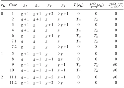
TABLE I. Patterns of conduction fornon-ipsomolecular devices, showing the total transmission,T(ϵK), the bond currentsJpAO→q(ϵK)calculated at the

shell eigenvalueϵK, and the shell currentJ_LMO→K(E)atanyenergy. The

non-zero quantitiesTa=B(qL,qR)ˆ02/|Dˆ0|2,Tb=B(qL,qR)βpqˆ0vˆpq ¯L ¯R,0/|Dˆ0|2, Tc=B(qL,qR)ˆ−21/|Dˆ−1|

2_{, and T}

d=B(qL,qR)βpqˆ−1vˆpq ¯L ¯R,−1/|Dˆ−1|2 are

evaluated using Eq.(58), subject to conditions implied bygt,gu, andgv

in the particular case.

rK Case gt gu gv gj T(ϵK) JpAO→q(ϵK) J_LMO→K(E)

0 1 g+1 g+1 g+2 ≥g+1 0 0 0 2 g+1 g+1 g g Ta Tb 0 3 g+1 g g+1 ≥g+1 0 0 0 4 g+1 g g g Ta Tb 0 6 g g g+1 g Ta Tb 0

7.1 g g g g Ta Tb 0

7.2 g g g ≥g+1 0 0 0 1 5 g+1 g−1 g ≥g 0 0 0 8 g g−1 g−1 ≥g 0 0 0 9 g−1 g−1 g g−1 Tc Td ,0

10 g−1 g−1 g−1 g−1 Tc Td ,0 2 11.1 g−1 g−1 g−2 g−1 0 0 ,0 11.2 g−1 g−1 g−2 ≥g 0 0 0

alone does not give access to full information aboutgjbut the

table included here does so, enabling some new sub-cases to be distinguished. The cases were previously stated in terms of the Fermi energy, but the analysis can be extended to the whole eigenvalue spectrum ofG.46

We re-examine these eleven canonical cases in detail in theAppendixaccording to the rank of the connection matrix,

Bcon

K , where it is shown that the eight possibilities for the

construction ofBcon

K in the echelon representation map onto

the eleven cases for conduction determined by interlacing. The results of this process are given in TableI, showingtotal

transmission, T, and bond currents JAO

p→q, both evaluated at

the shell eigenvalue,ϵK, and the shell current,JL→K, forany

energy. The property of inertness or activity of the shell can be read offfrom the final column of the table. An entry “,0”

means that the shell is active, and “0” means that it is inert. Overall conduction or insulation of the device is given by the entry in column 7 of the table.

The rank-0 cases in Table Ipossess the very important property that for all these cases the shell is insulating at all

energies, i.e., is inert. As far as conduction is concerned, it is as if the shell were not present. Any conduction at the eigenvalue predicted in that rank-0 case must, therefore, be carried through “off-shell” orbitals. This is very different from the normal behaviour, where an “active” shell carries all the transmission at its own shell eigenvalue.

The property of inertness is not particularly unusual nor is it restricted to degenerate shells. Indeed, TableIshows that all cases bar three (9, 10, and 11.1) of the possible eigenvalue combinations imply an inert shell.

The classification of case by rankrKmatches exactly the classification by Varieties in the mathematical treatment of Fermi-level conduction published elsewhere.47 We note that rank zero corresponds to Variety 3, rank one to Variety 2, and rank two to Variety 1. Devices that fall under cases 11.1 and 11.2 are based on uniform-core graphs described in Ref.47.

Two further remarks can be made about the applicability of this extended table, compared to that of Table I in Refs.31

and 35 which were limited to describing behaviour at the Fermi level for devices based on general and bipartite graphs, respectively. The first is about the interpretation of the present table for the case when all quantities are evaluated at a value, E, that is not an eigenvalue of G, i.e., when g=0. The formally allowed cases in TableI are then those with min_{gt−g, gu−g, gv−g}≥0, i.e., the cases

of rank rK=0. In such cases, the generic statements about

overall transmission (column 7) and bond currents (column 8) hold, provided all the quantities are evaluated by taking the structural polynomials at E. The shell current, JMO

L→K(E)

(column 9), has no meaning in this case.

The second remark is about the use of the extended table for devices based on bipartite graphs. When the table referred only toϵK=0, it was possible to use the special property that

the nullity and order of a bipartite graph have the same parity to reduce the number of cases from 11 to 5 (or from 13 to 6 in the finer classification used in the present paper). WhenϵK

is a general eigenvalue, the link between nullity and order is broken; deletion of a vertex of a bipartite graph may leave the degeneracy of a given eigenvalue unchanged, (or increased or decreased by one), and hence, any of the cases in TableImay apply.

E. Conduction inipsodevices

Devices where the external links are connected to the

sameinternal atom are termedipsodevices. In this case it is easy to see that we can take t=u= j, and v≡0, and it is clear that the connection matrix can have rank 0 or 1 only. In our treatment we consider that the parameters βL, β_LL¯ , and

βR, β_RR¯ have the same values as for non-ipso devices. The

expansion of ˆDbecomes

ˆ

D−2=0,

ˆ

D−1=− (

βLe−iqLβ2

¯ RR+βRe

−iqRβ2

¯ LL

)

ˆ

t−1,

ˆ

D0=βLe−iqLβ_Re−iqR₋(β_Le−iqLβ2

¯ RR + βRe−iqRβ2

¯ LL

)

ˆ

t0

(104)

ˆ

D−2vanishes becausev≡0.

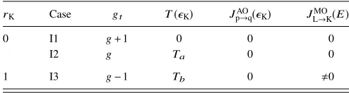
There are only three possible cases (cf. Table II) depending on the allowed gt values for the graph with

vertex ¯L removed. There is no restriction on the value of g.

TABLE II. Patterns of conduction foripsomolecular devices, showing the total transmissionT(ϵK), the bond currentsJpAO→q(ϵK)calculated at the shell

eigenvalueϵK, and the shell currentJ_LMO→K(E)atanyenergy. The non-zero

quantitiesTa=B(qL,qR)tˆ02/|Dˆ0|2andTb=B(qL,qR)tˆ2−1/|Dˆ−1|2are

evalu-ated using Eq.(104)for the particular case.

rK Case gt T(ϵK) JpAO→q(ϵK) J_LMO→K(E)

0 I1 g+1 0 0 0

I2 g Ta 0 0

1 I3 g−1 Tb 0 ,0

The cases exhibit all possible combinations of device conduction/insulation and shell character.

Case I1 (gt=g+1)

This case has a rank-0 connection matrix because ˆ

t−1=t0ˆ =0. The numerator incRisO(pK), whereas ˆD0is

the leading term in the denominator. HencecR=0 at the eigenvalue; there is device insulation and the shell is inert.

Case I2 (gt=g)

This case also has rank 0 because ˆt−1=0. As ˆt0,0,

and ˆD0 is the leading term in the denominator, there is

device conduction at the eigenvalue. However, the shell is inert, so conduction at this eigenvalue is carried entirely by orbitals from other shells.

Case I3 (gt=g−1)

This case has a rank-1 connection matrix, and is the equivalent of thenon-ipsocase 11. We have ˆt−1,0, and

so ˆD−1,0. The numerator and denominator have the

same order in pK, and device conduction occurs at the eigenvalue. The shell is active and carries all the current at the shell eigenvalue.

F. A difference between conduction of

ipso-andnon-ipso devices

The remaining feature of ipso devices is that the expressions for currents and total transmission depend upon the behaviour of a single structural polynomial. For this reason, the transmissionT₍E₎has zeros every time that ˆt₍E₎

vanishes. It is easy to see from the definition, Eq. (43), that ˆt(E) is a piecewise continuous curve with asymptotes at the molecular eigenvalues, and that the gradient is always negative. It follows that there will be a zero of ˆt(E)between each molecular eigenvalue (cf. Fig. 9). Consequently, ipso

transmission curves typically look very different from the curves fornon-ipsodevices based on the same molecule, cf. SectionIX.

VIII. CONDUCTION IN MOLECULES WITH BIPARTITE GRAPHS

An alternant molecule has a bipartite molecular graph containing two disjoint sets of nodes (atoms) and in which edges (bonds) connect only members of the two sets. We shall call these two setsS◦andS∗. If we number the members of the sets contiguously, then we can write the adjacency matrix in the form

A=*

, 0 B



B 0+

-, (105)

where we have placed then◦un-starred vertices in the first, and then∗starred vertices in the second block, and we assume that n◦≤n∗. The dimension of the matrix B is, therefore,

n◦×n∗.

A simple two-component SSP approach to conductivity in bipartite molecules has been developed26,48 for the case

E=0. In this section, we derive rules that apply to such molecules at general values ofE.

A. The Coulson-Rushbrooke theorem

For convenience, we present a compact derivation of this well-known49 theorem in a formalism that is useful for our study of conduction.

We can solve the eigenvector problem for the positive semi-definite matrix BB of dimension n_◦×n_◦ and of rank

r ≤n◦, in the form

BBVk=Vkσk2for k=1, . . . ,r,

BBV_k=0 for k=r+1, . . . ,n_◦,

(106)

where the n◦×n◦ matrix, V, formed from the n◦ columns

Vk is an orthogonal transformation with n◦−r null-space eigenvectors. We can also consider the n∗-dimensional eigenvalue problem



BBWk=Wkσ2kfor k=1, . . . ,r,



BBWk=0 for k=r+1, . . . ,n∗,

(107)

which has r identical positive eigenvalues, a null-space of dimension n∗−r, and the matrix Wis orthogonal. We can write thesingular value decompositionofBas

BW=VΣ

or



BV=WΣ, (108)

where the n◦×n∗ matrix, Σ is in principle rectan-gular, with a diagonal containing the positive numbers σ1≥σ2≥ · · · ≥σr>0.

We can now construct an ₍n◦+n∗)-dimensional orthog-onal transformation

*

,

V 0

0 W+

-(109)

that when applied to adjacency matrix Eq. (105) gives rise, for each of the r terms having σk>0, to a series of 2×2

interacting blocks of the form

*

, 0 σk

σk 0

+

-. (110)

These blocks are each diagonalised by the same 2-dimensional orthogonal transformation

*

, 1/

√ 2 1/

√ 2

1/ √

2 −1/ √

2+

-. (111)

The appropriate combination of Eqs. (109)and(111)solves the original eigenvalue problem by providing r paired solutionsψk,ψ¯khaving eigenvalues+σkand−σk, respectively,

and constructed from columns of the orthogonal matricesV

andW. They are

ψk=

1 √ 2

* .

,



p∈S◦ Vpkφp+



p∈S∗ Wpkφp+/

-,

ψ_¯k=√1 2

* .

,



p∈S◦ Vpkφp−



p∈S∗ Wpkφp+/

-(112)

for k=1, . . .r, and the nullspace is

ψk= 

p∈S◦

Vpkφpfor k=r+1, . . . ,n◦,

ψ_¯k∗=



p∈S∗

Wpkφpfor k∗=r+1, . . . ,n∗.

(113)

Hence, there are 2reigenvalues in pairs related to each other by a change of sign, and a nullspace of dimensionn◦+n∗−2r. This is the content of the Coulson-Rushbrooke pairing theorem.50–52 _{We now derive an extension for conduction} properties.

B. Structural polynomials for bipartite graphs

For bipartite graphs (alternant molecules), we can obtain structural polynomials from the above formulae for the eigenvectors and eigenvalues, together with the spectral expansions given earlier. Hence, after some algebra,

ˆ

t=E r



k=1 V_Lk¯2

E2₋σ2 k

+ 1 E

n◦



k=r+1

V_Lk¯2 for ¯L∈ S◦,

ˆ

t=E r



k=1 W2

¯ Lk E2₋σ2

k + 1

E n∗



k=r+1

W_Lk2¯ for ¯L∈ S∗.

(114)

The formulae for ˆuare easily obtained by analogy. It is seen that

ˆ

t₍−E₎=−tˆ₍E₎,

ˆ

u₍−E₎=−uˆ₍E₎, (115)

so that both functions are odd, as expected from parity arguments. The equations for ˆ are more complicated, as there are two cases, depending on whether indices ¯L,R belong¯ to the same or different sets. When ¯L∈ S◦and ¯R∈ S◦,

ˆ =E

r



k=1 V¯_LkV¯_Rk

E2₋σ2 k

+ 1 E

n◦



k=r₊1

V¯_LkV¯_Rk (116)

which is an odd function ofE. When ¯L∈ S◦and ¯R∈ S∗,

ˆ =

r



k=1

σk V¯_LkW_Rk¯

E2₋σ2 k

(117)

which is even. From the formula ˆv =uˆtˆ−ˆ2_{, it is clear that}

ˆ

v₍E₎=vˆ₍−E₎, regardless of the nature of ¯L and ¯R.

C. Conduction properties of alternant molecules

We now consider the transmission properties of molecules with bipartite graphs for unbiased devices, i.e., those for whichαL=αR=0, under the transformation E→ −E. This

transformation affects the momenta (cf. Eq. (6)) through

qL→ π−qL and qR→ π−qR. It follows that exp₍−iqL₎

→ −exp₍iqL₎, and sinqL→ −sinqL. The terms inqRbehave in an identical manner. From the discussion of the transformation properties of these quantities, it is obvious from Eq.(5)that

D(−E)=D(E)∗ (118)

and hence

T(−E)=T(E) (119)

so that the total transmission is symmetric about E=0 for unbiased devices.

We can also look at the symmetry properties of the MO currents by writing Eq.(83)in terms of the hatted polynomials,

J_LMO_→k(E)=B₍qL,qR)U¯LkU¯Rk E−ϵk

ˆ ₍E)

|Dˆ₍E_)|2. (120)

Putting this equation into the context of the current section: for the paired orbitals,ψk,ψ¯k, we recognise that the eigenvectors

for the paired MOs satisfy

Upk=Up ¯k for p∈ S◦,

Upk=−Up ¯kfor p∈ S∗,

(121)

and

J_LMO_→k(E)=J_LMO_→¯k(−E). (122)

The paired orbitals have currents that are reflections of each other about the line E=0. It is also obvious that Eq. (122)

forg ≥2 extends also to shells, so that

J_LMO_→K(E)=J_LMO_→K¯(−E). (123)

It can be shown that bond currents in bi-partite molecules also display the same symmetry,

J_pAO_→q(E)=J_pMO_→¯q(−E). (124)

D. Conduction at the Fermi level

We now turn to the conduction properties of the shell at ϵk=0. The conduction properties can be discussed in a very

simple manner using the eigenspaces listed in Eqs.(112)and

(113), and the connection matrix in Eqs.(31)and(34). For molecular graphs that possess a nullspace, we have a single shell with ϵK=0 and degeneracyg =n◦+n∗−2r. There are two possibilities.

1. Contact atoms in different sets, e.g., ¯L∈ S◦and ¯R∈ S∗. In this case, the structure of thenull-spaceconnection vector is

uL= βLL¯

* . . . . . . . . . . . . . ,

V¯Lr+1

.. .

V¯_Ln◦

0 .. . 0 + / / / / / / / / / / / / /

-,uR=βRR¯

* . . . . . . . . . . . . . , 0 .. . 0

W_R¯r₊1

.. .

WR¯n∗

+ / / / / / / / / / / / / / -. (125)

The formula for MO currents, Eq.(83), shows that current is proportional to a product of ¯L and ¯R MO coefficients from the connection vectors. The structure of the vectors in Eq.(125) implies that this product is identically zero. The shell carries no current and is inert regardless of the rank of the connection matrix.

2. Contact atoms in the same set, e.g., ¯L∈ S_◦and ¯R∈ S_◦.

In this case, the structure of thenull-spaceconnection vector is

uL= βLL¯

* . . . . . . . . . . . . . ,

V¯Lr+1

.. .

V¯_Ln◦

0 .. . 0 + / / / / / / / / / / / / /

-,uR=βRR¯

* . . . . . . . . . . . . . ,

V¯Rr+1

.. .

V¯_Rn◦

0 .. . 0 + / / / / / / / / / / / / / -. (126)

The n∗−r molecular orbitals from the starred space are all inert, but the MOs from the un-starred space are not necessarily inert. The shell may therefore still be active, depending on the case to which the shell belongs (cf. TableI).

For cases where E=0 is notan eigenvalue, the present reasoning makes a connection with a “symmetry rule” (actually a graph-theoretical rule) for non-ipso conduction at the Fermi level for closed-shell alternant molecules.42,53 It was observed that the predicted Fermi-level conduction of a molecule with bipartite molecular graph and a non-zero HOMO-LUMO gap (specifically a Kekulean benzenoid) is large when both HOMO and LUMO have entries of large magnitude on both connection vertices (our ¯L and ¯R) and the product of entries is of opposite sign for HOMO and LUMO. By the pairing theorem, this latter requirement implies that the connection vertices are in different partite sets.

This rule has a straightforward interpretation in terms of shell contributions. HOMO and LUMO shells of a bipartite graph have mirror conduction curves, so are either both active or both inert. For active shells, both shell conduction curves will be close to local maxima in the vicinity of the Fermi level. If the connection vertices are in opposite sets, the curves will contribute equal amounts to the total conduction at the Fermi level. (Other active shells will typically also contribute. Such contributions may be positive or negative.) If the connection vertices belong to the same partite set, however, we have nullity signatureg=0, gt =gu=1,gv=2 and insulation at

the Fermi level.31

IX. SOME ILLUSTRATIVE EXAMPLES

We illustrate our description of molecular conduction with a proof that every molecular graph has at least one active shell, then some analytical examples for chains and rings, and finally some more general molecular examples.

A. Molecular conduction of LOMO and HUMO shells

Everyπsystem with a connected molecular graphGhas a non-degenerate lowest-lying π level. Mathematically, the eigenvector corresponding to the largest positive eigenvalue of

G,ϵmax, i.e., the lowest occupiedπmolecular orbital (LOMO),

has specific implications for the conduction properties. This maximum eigenvalue is known as the Perron eigenvalue; it has multiplicity one for a connected graph, and the associated eigenvector has a non-zero entry of the same sign on every