Optimal test signal design and estimation for dynamic powertrain calibration and control

(1)

Optimal Test Signal Design and

Estimation for Dynamic Powertrain

Calibration and Control

Thesis submitted in accordance with the requirements of the

University

of

Liverpool

for the

Degree of Doctor in Philosophy

by

Ke Fang

(2)

Statement of Originality

This thesis is submitted for the degree of Doctor in Philosophy in the Faculty of

Engi-neering at the University of Liverpool. The research project reported herein was carried out,

unless otherwise stated, by the author in the Department of Engineering at the University of

Liverpool between October 2008 and October 2011.

No part of this thesis has been submitted in support of an application for a degree

or qualiﬁcation of this or any other University or educational establishment. However, some

parts of this thesis have been published, or submitted for publication, in the following papers:

• K. Fang and A.T. Shenton, Optimal Input Design for Dynamic Engine Mapping, 6th

IFAC Symposium Advances in Automotive Control, Munich, Germany, 2010

• K. Fang and A.T. Shenton, Optimal Test Signal Design for the Identiﬁcation of

Dynam-ic Engine Model, 1st International Conference on Powertrain Modelling and Control,

Bradford, UK, 2012

• A.T. Shenton and K. Fang, IC Engine Dynamic Calibration and Control by Inverse

Op-timal Behaviours, 1st International Conference on Powertrain Modelling and Control,

Bradford, UK, 2012

• K. Fang and A.T. Shenton, Optimal Input Design for Dynamic Model Prediction

Ac-curacy, 15th IFAC Workshop on Control Applications of Optimization, Rimini, Italy,

2012

• K. Fang and A.T. Shenton, Constrained Optimal Test Signal Design for Improved

Pre-diction Error,submitted to IEEE Transaction on Automation Science and Engineering,

October, 2012

Ke Fang

30th November 2012

(3)

Abstract

With the dramatic development of the automotive industry and global economy, the motor

vehicle has become an indispensable part of daily life. Because of the intensive

competi-tion, vehicle manufacturers are investing a large amount of money and time on research in

improving the vehicle performance, reducing fuel consumption and meeting the legislative

requirement of environmental protection. Engine calibration is a fundamental process of

de-termining the vehicle performance in diverse working conditions. Control maps are developed

in the calibration process which must be conducted across the entire operating region before

being implemented in the engine control unit to regulate engine parameters at the diﬀerent

operating points. The traditional calibration method is based on steady-state (pseudo-static)

experiments on the engine. The primary challenge for the process is the testing and

opti-misation time that each increases exponentially with additional calibration parameters and

control objectives.

This thesis presents a basic dynamic black-box model-based calibration method for

multi-variable control and the method is applied experimentally on a gasoline turbocharged direct

injection (GTDI) 2.0L virtual engine. Firstly the engine is characterized by dynamic models.

A constrained numerical optimization of fuel consumption is conducted on the models and the

optimal data is thus obtained and validated on the virtual system to ensure the accuracy of

the models. A dynamic optimization is presented in which the entire data sequence is divided

into segments then optimized separately in order to enhance the computational eﬃciency. A

dynamic map is identiﬁed using the inverse optimal behaviour. The map is shown to be

capable of providing a minimized fuel consumption and generally meeting the demands of

engine torque and air-fuel-ratio. The control performance of this feedforward map is further

improved by the addition of a closed loop controller. An open loop compensator for torque

control and a Smith predictor for air-fuel-ratio control are designed and shown to solve the

issues of practical implementation on production engines.

A basic pseudo-static engine-based calibration is generated for comparative purposes

and the resulting static map is implemented in order to compare the fuel consumption and

torque and air-fuel-ratio control with that of the proposed dynamic calibration method.

Methods of optimal test signal design and parameter estimation for polynomial models

are particularly detailed and studied in this thesis since polynomial models are frequently

(4)

used in the process of dynamic calibration and control. Because of their ease of

implemen-tation, the input designs with diﬀerent objective functions and optimization algorithms are

discussed. Novel design criteria which lead to an improved parameter estimation and output

prediction method are presented and veriﬁed using identiﬁed models of a 1.6L Zetec engine

developed from test data obtained on the Liverpool University Powertrain Laboratory.

Prac-tical amplitude and rate constraints in engine experiments are considered in the optimization

and optimal inputs are further validated to be eﬀective in the black box modelling of the

virtual engine. An additional experiment of input design for a MIMO model is presented

based on a weighted optimization method.

Besides the prediction error based estimation method, a simulation error based

esti-mation method is proposed. This novel method is based on an unconstrained numerical

optimization and any output ﬁtness criterion can be used as the objective function. The

eﬀectiveness is also evaluated in a black box engine modelling and parameter estimations

with a better output ﬁtness of a simulation model are provided.

(5)

Acknowledgments

I would like to show my gratitude to my supervisor Dr. Tom Shenton for his guidance

and support in the completion of this work. It was not possible to ﬁnish this project without

his great help. I owe a thanks to Dr. Paul Dickinson for his indispensable assistance in the

experimental setup. I would also like to thank all my friends: Shiyu Zhao, Ahmed Abass,

Zongyan Li, Mingyen Chen and Ziyun Ding for their advice in discussions.

Thanks to my wife Meirong and my parents for their inspiration and encouragement

dur-ing the undertakdur-ing of this work and thanks to ORSAS and Hong Kong Graduate Association

Awards for their ﬁnancial support.

(6)

List of Figures

1.1 A procedure of model-based static calibration [1] . . . 6

1.2 A schematic conﬁguration of a PFI IC engine [2] . . . 7

1.3 Engine emissions after the TWC with diﬀerentλ[3] . . . 10

1.4 Emission and fuel consumption in SA sweeping [3] . . . 11

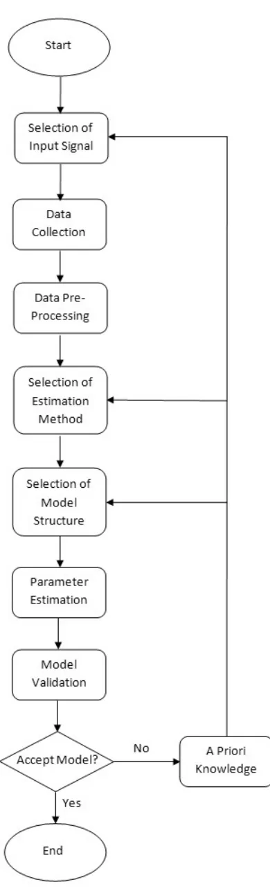
2.1 A general procedure of system identiﬁcation . . . 16

2.2 Overview of DoE optimality-criteria . . . 20

2.3 Structure of ARX model . . . 26

2.4 Structure of ARMAX model . . . 27

2.5 Structure of OE model . . . 27

2.6 Structure of BJ model . . . 28

2.7 Schematic of a neuron . . . 33

2.8 Schematic of a single layer . . . 34

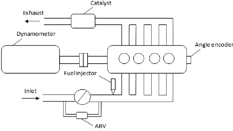
3.1 A schematic of the engine setup and key instrumentation . . . 38

3.2 Hardware and software conﬁguration of engine experiments . . . 39

3.3 An example of simulating a cylinder by WAVE . . . 40

3.4 WAVE virtual engine . . . 41

3.5 SI Wiebe combustion model . . . 42

3.6 WAVE virtual engine with sensors and actuators . . . 44

3.7 WAVE-RT block . . . 45

3.8 Adapted WAVE-RT model of the virtual engine . . . 46

3.9 Forces on a wheel in motion . . . 49

3.10 Simulink model of the autogear subsystem . . . 51

3.11 Simulated vehicle speed and engine speed in acceleration . . . 51

4.1 Schematic of the convex (top) and nonconvex (bottom)optimization . . . 56

4.2 Flow chart of the iterative process of optimal input design . . . 62

4.3 ACFRu(L) and PSDSu(ω) of an ideal white noise . . . 63

4.4 Simulated white noise and ACF . . . 64

(12)

4.5 Discrete random binary signal and corresponding ACF . . . 64

4.6 A Simulink generator of PRBS . . . 65

4.7 ACF of PRBS . . . 65

4.8 A Simulink generator of APRBS . . . 66

4.9 A Simulink generator of amplitude constrained random walk signal . . . 67

4.10 Normal distribution of estimated parameter ˆθj . . . 72

4.11 UDRN input and optimal input . . . 74

4.12 Objective function value by local algorithms . . . 75

4.13 Current function value and best function value by simulated annealing . . . . 76

4.14 Objective function value by genetic algorithm . . . 77

4.15 Objective function value and mesh size of pattern search . . . 77

4.16 Distribution of estimated parameter ˆθ(1) . . . 82

4.17 U0 selection in a closed loop control system . . . 86

4.18 Procedure of building model pool and validation . . . 90

4.19 An example of test signals of diﬀerent types . . . 91

4.20 An example of the rate constrained random walk signal and optimal signals . 97 4.21 Measured output and simulated output of black box torque model . . . 100

4.22 An example of UDRN signal and optimal signal . . . 101

5.1 Schematic of simulation model and prediction model . . . 106

5.2 Measured output and predicted output . . . 109

5.3 Measured output and simulated output by PEM . . . 110

5.4 Minimized objective function value by Pattern Search method . . . 111

5.5 Measured output and simulated output by SEM . . . 113

6.1 Schematic of a calibrated control system . . . 118

6.2 Simpliﬁed conﬁguration of the WaveRT model for initial development . . . . 119

6.3 Model operating envelope and reduced calibration region . . . 121

6.4 Throttle (a) and fuel mass (b) required to maintain torque demand . . . 122

6.5 Calibration maps of the reduced region (a) and low-speed low-load region (b) 123 6.6 Optimal input signals at random operating points . . . 125

6.7 Optimal engine outputs at random operating points . . . 126

6.8 Optimal engine outputs with optimal SA and random SA . . . 126

7.1 Basic dynamic calibration and control conﬁguration . . . 131

7.2 The process of dynamic calibration and control . . . 133

7.3 A proﬁle of engine speed at the acceleration of vehicle . . . 137

7.4 Series-parallel architecture (a) and parallel architecture (b) . . . 139

(13)

7.5 The architecture of selected NARX neural networks . . . 140

7.6 Simulated engine outputs and real engine outputs . . . 140

7.7 Validation of NN and polynomial models . . . 143

7.8 The eﬀect of segment approach on output constraints . . . 147

7.9 A schematic of the predictive horizon approach . . . 147

7.10 The eﬀect of predictive horizon approach on output constraints . . . 148

7.11 An example of the eﬀect by input smoothing on the outputs . . . 149

7.12 Optimal inputs obtained by constrained fuel optimization . . . 150

7.13 Demanded constraints and optimal outputs on NN models . . . 151

7.14 Optimal outputs on NN model and RT model . . . 152

7.15 Optimal outputs on RT model by iterations . . . 153

7.16 Optimal SA obtained with/without rate constraint . . . 154

7.17 Optimal outputs on RT model with/without rate constraints . . . 155

7.18 A Schematic of feedforward controller . . . 156

7.19 Optimal inputs and simulated optimal inputs by inverse models . . . 158

7.20 Control performance of dynamic map in oﬄine validation . . . 159

7.21 Control performance of the dynamic map and static map in online validation 160 7.22 The Bode plot of frequency responses in 4 channels . . . 162

7.23 The parameter plane of P and I terms . . . 163

7.24 Closed loop control performance of PI controllers . . . 164

7.25 An open loop compensator for torque control . . . 164

7.26 Closed loop control performance of an open loop compensator . . . 166

7.27 A Smith predictor for system with extra output time delay . . . 167

7.28 A Smith predictor for λcontrol . . . 168

7.29 Closed loop control performance of PI controllers in delayed system . . . 168

7.30 Closed loop control performance of Smith predictor in delayed system . . . . 169

7.31 Optimal outputs on the RT model (segment length of 100 points) . . . 170

7.32 Optimal outputs on the RT model (segment length of 500 points) . . . 171

7.33 Optimal inputs and simulated optimal inputs by inverse models . . . 172

7.34 Closed loop control performance of PI controllers . . . 172

7.35 Control performance of dynamic maps in online validation . . . 174

9.1 A schematic of multi-models . . . 184

(14)

Abbreviation

ABV Air-Bleed Valve

ACF Auto-Correlation Function

AFR Air-Fuel Ratio

AIC Akaikes Information Criterion

APRBS Amplitude modulated Pseudo-Random Binary Sequence

ATDC After Top Dead Centre

ARMAX AutoRegressive Moving Average with eXogeneous inputs

ARX AutoRegressive with eXogeneous inputs

BDC Bottom Dead Centre

BIC Bayesian Information Criterion

BJ Box-Jenkins

BTDC Before Top Dead Centre

DoE Design of Experiment

ECU Engine Control Unit

EGR Exhaust Gas Recirculation

EMS Engine Management System

FPE Final Prediction Error

FPW Fuel Pulse Width

GA Genetic Algorithm

GDI Gasoline Direct Injection

GTDI Gasoline Turbocharged Direct Injection

HEGO Heated Exhaust Gas Oxygen

IC Internal Combustion

INJ INJected fuel mass

IP Interior Point

MIMO Multiple-Input-Multiple-Output

MISO Multiple-Input-Single-Output

MLE Maximum Likelihood Method

MSE Mean Squared Error

NARX Non-linear AutoRegressive with eXogenous inputs

NN Neural Network

OE Output Error

OLS Ordinary Least Square

PEM Prediction Error Method

PFI Port Fuel Injection

PRBS Pseudo Random Binary Sequence

PS Pattern Search

(15)

PSD Power Spectral Density

RBS Random Binary Signal

RPM Revolutions Per Minute

RT Real Time

SA Spark Advance

SAN Simulated ANnealling

SEM Simulation Error Method

SI Spark Ignition

SISO Single-Input-Single-Output

SQP Sequential Quadratic Programming

TDC Top Dead Centre

TRR Trust Region Reﬂective

TWC Three Way Catalyst

UDRN Uniformly Distributed Random Number

UEGO Universal Exhaust Gas Oxygen

(16)

Chapter 1

Introduction

In recent years advanced technologies have been introduced to further reduce the fuel

con-sumption and emissions of vehicles. These technologies require complex and expensive engine

calibration work. With traditional hardware-based calibration methods, the experimental

time increases signiﬁcantly with additional calibration parameters and may not include

im-portant transient characteristics of the system.

Dynamic models and dynamic model-based calibration are thus being investigated, which

are able to capture the dynamic behaviour and possibly decrease the cost of calibration by

a reduction of set-points and settling time. Dynamic models can also incorporate

data-smoothing into the model structure and integrate the calibration and control processes. As

more calibration work is carried out on models rather than the real engine the requirement

for model quality is essential. In this thesis methodologies of experiment design and model

estimation are accordingly proposed to improve the accuracy of identiﬁed dynamic models

required for calibration optimisation and system identiﬁcation.

1.1 Advanced Technologies of Gasoline Engines

The gasoline engine has always been the most widely used type of engine in the automotive

industry since the ﬁrst development of the car. Although its performance has been constantly

improved by continuous research over decades, there is still a large potential for further

improvement by using model-based control technologies [2]. Advanced automotive engine

technologies are being increasingly implemented in order to satisfy the customer demands

on fuel economy and also the legislative requirements on scheduled emissions. Many new

technologies have already been made commercially available and utilized in production. These

are summarized in the following sub-sections.

(17)

CHAPTER 1. INTRODUCTION 2

1.1.1 Variable Valve Timing

The inlet and exhaust valves control the amount of air ﬂow going into or out of the cylinder

therefore the control of valves has a signiﬁcant inﬂuence on the combustion and volumetric

eﬃciency and so the resulting engine performance. In gasoline engines, the valves are driven

by a camshaft which is normally connected to the crankshaft through the timing belt, and

the opening and duration are determined correspondingly. For early engines in which the

phasing of the camshaft was ﬁxed, it was not possible to alter the timing under changing

operating conditions so that the engine performance and fuel economy were necessarily a

tradeoﬀ between low-load low-speed conditions and high-load high-speed conditions. For

instance a long opening at low engine speed will result in low fuel eﬃciency and increased

emission since the fuel may leave the combustion chamber without a full combustion.

Con-versely it will be beneﬁcial at high speed because of the less restriction on the air ﬂow [4].

Moreover, the requirement for high-power during a drastic changing in speed cannot be well

satisﬁed by traditionally ﬁxed valve timing which was designed for optimal performance in

high speed and high load conditions for maximum power. In recent decades the optimization

tends to focus on low speed and low load because of the requirement for fuel eﬃciency and

emission evoked by the concerns for oil supply and environmental protection.

Variable Valve Timing (VVT) refers to technologies which have the ability to adjust

the scheduled valve timing ﬂexibly in order to meet the desired performance in the various

operating regions. These technologies have been implemented by many automobile companies

and can be classiﬁed into four categories based on the controlled valves: phasing the inlet or

exhaust valves only; phasing the inlet and exhaust valves equally or independently. To realize

the variable timing, a mechanism that provided more than two cam proﬁles on the camshaft

was proposed ﬁrstly in the Honda VTEC[5]. The driving cam was switched alternatively

according to the engine speed. More recently, technologies of VVT for camless engine have

been developed [6, 7]. The valves are directly controlled by an electromagnetic or hydraulic

approach. This approach allows a continuous control depending on key control references

such as torque and engine speed hence it is capable of obtaining optimal engine performance

in diﬀerent driving conditions. Nevertheless both electromagnetic and hydraulic valves need

additional energy which will correspondingly reduce the fuel eﬃciency. The real-time control

required by these various schedules raises the requirement for accurate and fast data collection

for model development to support the more complex control system.

VVT has an eﬀect which can reduce the fuel consumption and emissions. Normally the

optimal timing of the inlet valves helps to increase volumetric eﬃciency so that the maximum

torque for otherwise ﬁxed parameters in the whole operating region can be improved which

in turn increases the eﬃciency and fuel economy [8]. Eﬀects from the timing of the exhaust

(18)

CO and NOx [9]. A detailed review and analysis of various strategies for VVT control is

presented in [10, 11].

1.1.2 Gasoline Direct Injection

The technology of gasoline direct injection (GDI) has been an important innovation in

auto-mobile powertrain design in the last decade. In conventional port fuel injection (PFI) engines,

the fuel injector is located in the inlet manifold outside the inlet valve of each cylinder. The

injected fuel is ﬁrstly mixed with the air stream and then vaporized in the inlet port by the

impact with the top surface of the inlet valve and then enters the combustion chamber with

the opening of the valve. One of the associated disadvantages is that a fuel puddle is formed

in the inlet port, also known as wall wetting which will compromise the accurate control of

the fuel delivery and thus the fuel economy. Furthermore the resulting delay in fuel delivery

may lead to misﬁre or rich combustion especially in cold-start [12].

GDI has totally solved the issue of wall wetting by injecting the fuel directly to the

cylinder. Although the associated time between injection and ignition for mixture

prepara-tion is considerably reduced, the fuel spray can be well atomized within the time limit by

using a high pressure injector. The amount of fuel in each combustion event thus can be

ac-curately measured and controlled in diﬀerent working conditions of the engine and excessive

fuel supply is avoided. GDI provides the potential for implementing more complex control

methodology. As the timing of GDI is independent of the valve timing, the engine

manage-ment system (EMS) allows for multi-combustion models: stratiﬁed charge and homogeneous

charge. Stratiﬁed charge is selected in low-speed low-load conditions in which the engine

often experiences a constant speed or deceleration. A small amount of fuel is injected at the

end of compression stroke so that the lean mixture is away from the cylinder wall when

igni-tion happens. By reducing the wall heat loss, the thermal eﬃciency is signiﬁcantly improved

and the fuel economy enhanced accordingly. However, since the lean burn causes emission

issues, a stoichiometric air-fuel ratio is required in most conditions. The fuel is injected in the

intake stroke and the homogenous mixture leads to an exhaust gas which can be eﬀectively

converted by the catalyst.

Besides the major advantage in fuel economy, the merit of GDI is extended to emission

control since the rich air-fuel ratio (AFR) caused by the generation of a fuel puddle in

the cold-start is avoided; It is also beneﬁcial in improving the transient response as less

acceleration-enrichment for the puddle is required. A comprehensive comparison of PFI and

(19)

1.1.3 Turbocharger

Volumetric eﬃciency refers to the ratio of the air on real fuel-air mixture inducted into the

cylinder in each combustion event to that of the naturally aspirated engine at almost zero

engine speed. It is a key criterion of the performance of internal combustion engines since

it aﬀects the maximum achievable power in a unit of a given capacity. Devices such as

superchargers and turbochargers induct compressed air ﬂow, also known as forced induction,

to the cylinder and hence the associated allowable mass of fuel increases and more power can

be generated in each combustion.

The power supply required for the associated additional compression is the major

dif-ference between a supercharger and turbocharger. A supercharger is directly connected and

driven by the engine mechanically so that it has natural advantages of quick response to the

working condition and a reliable power supply. Nevertheless since a part of the generated

power needs to be used to maintain the running of the charger, this system may have

rela-tively low eﬃciency [16]. On the other hand, a turbocharger is driven by the energy of the

exhaust gas which was not utilized although it will increase the back-pressure. This system

is composed of a turbine and compressor. The exhaust gas delivered into the turbine is

con-trolled by a waste gate which is capable of diverting the gas away from the compressor. The

boost-pressure of the intake manifold is thus regulated and the risk of damaging the engine

due to eﬀects such as knock can be consequently reduced. Turbochargers provide a

signiﬁ-cantly enhanced power in high speed conditions however they work much less eﬃciently at

low speed conditions because the amount of exhaust gas is insuﬃcient to spin the compressor

to boost. Another challenge of this system is the turbo lag. Due to the basic mechanism

of the turbocharger, the time required to generate the boost results in a time delay in the

response to changes in working conditions. Correspondingly undesirable drivability issues

might be caused in any accelerations.

A twincharger is a compound system composed of supercharger and turbocharger, which

can solve the defects of each type of forced induction system eﬀectively. This technology has

been successfully implemented in several types of production car, such as the 125 kW 1.4 litre

turbocharged stratiﬁed injection engine [17], but the disadvantages of the high cost of the

components and the requirement for extremely accurate control raise new barriers to their

adoption.

1.2 Engine Calibration Methodologies

Along with the development of mechanical and electronic technologies, the methodologies of

(20)

of engine development, the engine calibration determines optimal settings for the best overall

engine performance in the various operating conditions. In early times, calibrations were

directly carried out on the engine while in modern times the development is moving towards

model-based or simulation-based methods because of the rapidly increasing complexity.

Conventional calibration methods which have been used worldwide are based on

pseudo-static testing on the real engine over the entire operating range. Since the experiments are

conducted directly on the engine, the results obtained from the test bed are considered

ac-curate and reliable enough for implementations on current production vehicles. Nevertheless

this method has also been criticized for its ineﬃciency in testing and optimization [18]. In

general, all inputs need to be swept in order to ﬁnd the optimal point at each operating point

and therefore a large number of experiments is unavoidable. Due to the nature of

steady-state testing, it is necessary to wait for the output response to reach a steady steady-state which

in turn further increases the required experimental time. Moreover with the development

of advanced engine technologies, more engine parameters and variables including valve

tim-ing and waste gate timtim-ing become controllable and the associated dimension of experiments

increases signiﬁcantly.

Model-based calibration methods have been developed to reduce the cost of experiment

[19]. A global model or local models are identiﬁed from engine data in the operating regions

and then used as a replacement of the real engine for oﬄine calibration and optimization

which takes the majority of the online calibration burden out of the engine test bench and

into a PC. The accuracy of models is a crucial factor since it signiﬁcantly aﬀects the

eﬀec-tiveness of optimal settings for the controllers which should be robust to the uncertainty in

the models. The beneﬁt in reduced experimental cost from employing model-based

calibra-tion has popularised these methods which mainly include static and dynamic model-based

calibration methods.

1.2.1 Static Modelling and Mapping

Figure 1.1 demonstrates a typical static model-based calibration approach. “Minimap” points

denote representative local operating points. Local tests are made at each point and

steady-state data is collected for the identiﬁcation of static models. Subsequent experiments for

determining the optimal settings are carried out on the resulting mathematical models and

local optimal settings are used to form calibration maps for the whole operating region. In

general the derived model is able to generate the simulated result in a short time hence the

settling time required in engine tests can be substantially reduced. As the data for analysis

is recorded in the steady state, the transient behaviour of the system is neglected so that

(21)

[image:21.612.116.527.63.316.2]

Figure 1.1: A procedure of model-based static calibration [1]

such as acceleration or deceleration.

1.2.2 Dynamic Modelling and Mapping

To capture the important dynamics of the system, dynamic modelling and mapping can be

employed. In the design of experiments (DoE), test signals should be appropriately designed

in order to excite the system dynamics and the input-output data are collected for model

estimation. Dynamic models describe the system behaviour by using the current and past

values of inputs and outputs so that they are capable of describing the transient response of

inputs and outputs. This approach also gives a potential for removing the burden of selecting

operating points and local testing at each point since a well designed dynamic model using

a clustering algorithm is able to simulate outputs at diﬀerent operating points with good

accuracy [20]. In the dynamic optimization, it may be possible to use the optimal settings

to identify a model which would interpolate and extrapolate to predict the optimal values

across a dense set of operating points.

Modelling and control of dynamic systems have been studied by many authors [21, 22,

(22)

[image:22.612.122.527.64.308.2]

Figure 1.2: A schematic conﬁguration of a PFI IC engine [2]

1.3 Engine Control

The obtained optimal settings are used to construct a calibration map in the form of look-up

tables and are stored in an engine control unit (ECU). The EMS collects the inputs from

engine sensors, searches for the stored settings and controls the actuators in real time to

produce the optimal performance. Figure 1.2 illustrates a simpliﬁed hardware conﬁguration

of a PFI Internal Combustion(IC) engine.

The entire control system often includes a large number of feedforward and feedback

control loops that are used to satisfy increasing performance requirements. The best engine

performance in terms of smooth response and powerful output with the least fuel consumption

has always been the top requirement of customers and automotive manufacturers. Meanwhile

legislation for environmental protection encourages the technological progress to address the

requirement of reducing vehicle emission. These requirements can only be satisﬁed by the

use of new electronic and mechanical automotive mechanism and control technology.

1.3.1 Torque Control

Engine torque is a vital characteristic of engine performance, which represents the power

generated in a fuel combustion for a given speed. In a production car it is closely related to

(23)

by a coupled dynamometer. On a production car, however it is not usually possible to measure

torque directly except with very expensive test instrument and normally it is estimated by a

model obtained from oﬄine experiments. Engine torque is determined by the combustion of

the air-fuel mixture in the cylinders consequently it can be controlled in two ways. As the

throttle angle aﬀects the intake air ﬂow which in turn determines the allowable fuel injection

and the mass of mixture, control of throttle is a common and eﬀective approach of regulating

engine torque in the spark ignition (SI) engine although it generates additional pumping

losses. Originally, the acceleration pedal was mechanically connected to the throttle so that

the driver could directly adjust the torque in a simple and quick manner. Alternatively,

now an electronic throttle control converts the signal of the pedal position into a desired

power output and the ECU will select or calculate coordinated optimal settings of all related

actuators accordingly. This technique provides a more ﬂexible and precise control. However

the transient response might be slower than the conventional mechanical control since the

throttle plate is adjusted by ﬁltered signals derived from feedback controllers in the ECU.

Combustion control is the major factor in transferring the chemical energy of the fuel into

kinetic energy therefore it also has a critical inﬂuence on engine torque. In a spark-ignition

IC engine, the spark advance (SA) angle needs to be optimized for maximum eﬃciency of the

combustion. The ignition causes an increase in in-cylinder pressure which creates the piston

work. A very early spark in the compression stroke will waste the energy required to push

the piston and will unnecessarily heat the cylinder wall. On the other hand, more energy

will be lost in the gas out of the cylinder in the exhaust stroke rather than being used to

accelerate the crankshaft if a too late spark occurs [3].

The main task of torque control is for the generated torque to track the desired torque

proﬁle, in which both accurate steady-state values and rapid transient responses are

com-monly required. Since the speed is relatively slowly changing and this is perceived by the

driver, the torque and power control are equivalent from the driver’s perspective. In practice

the need for high steady-state accuracy of torque is not great since the driver can manually

compensate the error by feedback compensation using the accelerator pedal. An open loop

control with an acceptable settling time may have the potential of satisfying the requirement

for good torque control.

1.3.2 Fuel Control

According to the ECU map settings, for any speciﬁc demand of torque the fuel consumption

may vary and so the best fuel economy must be obtained by an optimized fuel controller. As

mentioned above, the timing of spark is an essential factor since it determines the location

(24)

advanced engine technologies are introducing more factors in the fuel optimization. Variable

valve timing promotes the fuel eﬃciency by controlling the inlet valve. The overlap between

intake and exhaust valve is extended by early intake valve opening and consequently the burnt

high pressure and temperature gases will be pushed back to the intake manifold and sucked

into the cylinder in the next cycle and therefore the pumping losses are reduced. Early valve

closing happens when the desired amount of mixture is introduced in the cylinder so that

the required work for pumping is minimized. As gasoline direct injection (GDI) technology

can eliminate the fuel puddle in the conventional PFI engine, the compensation for the fuel

ﬁlm dynamics is not needed. The ﬂexible injection time control in GDI provides a further

potential for fuel reduction in low-speed low-load condition. The exhaust gas recirculation

and turbocharger can also contribute to the fuel eﬃciency by reducing the cylinder volumetric

capacity through utilizing the energy of the exhaust gas.

Idle speed speciﬁes a special low-speed low-load condition in which the fuel is consumed

only to prevent the stall of the engine. In order to reduce the fuel consumption, the rotational

speed of engine is expected to be as low as possible but still capable of maintaining the smooth

engine performance whilst still operating the ancillaries. Since approximately one third of

the fuel is consumed in idle speed because of the traﬃc congestion [25], the development of

an eﬃcient idle speed controller will make a signiﬁcant contribution to the fuel economy.

1.3.3 Air-Fuel Ratio Control

An eﬀective and eﬃcient after-treatment system is essential to satisfy the increasing legislative

requirement for the reduction of emissions. The converting eﬃciency of the three way catalyst

(TWC) is mainly aﬀected by the AFR and the AFR is normally desired to be stoichiometric,

usually about 14.7:1 orλ= 1, to ensure the optimal performance of the TWC [26]. As shown

in Figure 1.3, for a SI engine the main poisonous substances, NOx, CO and HC of vehicle

exhaust can be majorly ﬁltered by the TWC only if the λis in a narrow window around 1.

Hence the air-fuel ratio control is the most important feedforward and feedback control for

the regulation of emissions.

In common practice, an oxygen sensor is placed in the collective exhaust pipe before

the TWC. Instead of directly measuring mass of air and fuel in the mixture, this sensor

measures the proportion of oxygen and the AFR is determined accordingly [3]. A second

λsensor positioned after the TWC as in Figure 1.2 is used to monitor the eﬃciency of the

TWC. A typical widely used oxygen sensor is the heated exhaust gas oxygen (HEGO) sensor.

Although the HEGO sensor beneﬁts from its low cost, its output voltage is quite nonlinear

to the AFR. The resulting output voltage changes drastically around stoichiometric while

(25)

[image:25.612.196.455.64.305.2]

Figure 1.3: Engine emissions after the TWC with diﬀerent λ[3]

relatively poor for control purpose and its use is limited to limit-cycle control. An alternative

choice is the universal exhaust gas oxygen (UEGO) sensor which is capable of measuring the

AFR linearly across a wide range and therefore it is generally preferred in the test bench

since linear control technologies can be applied. However the high price of UEGO aﬀects its

implementation in production cars.

As can be seen from Figure 1.3, the emission rates of the exhaust gas varies and the high

conversion eﬃciency is achieved only within a very small window around the stoichiometric

point therefore a precise control of AFR in static and transient situations is required. To

design a feedforward controller, the dynamics of the intake air-path must necessarily be

es-timated in order to predict a suitable fuel ﬂow in the next engine cycle corresponding to the

related engine signal e.g. throttle position and SA. However for the purpose of reducing the

steady-state oﬀset to an acceptable limit, developing a model with required global accuracy

in the operating region is excessive time consuming. In order to eliminate the steady-state

er-ror, closed loop control can be employed. However the biggest challenge of adapting feedback

control is the long time delay caused by the transport delay associated with delivering the

raw exhaust gas from the actuator, which is usually the fuel injector, to theλsensor.

Con-sequently a combined feedforward-feedback control will be needed to overcome the defects

of each control method. With the implementation of certain advanced engine technologies,

the control system design can be simpliﬁed. For instance in conventional PFI engines, the

inﬂuence of fuel puddle and the time delay between the fuel injection and inlet valve opening

(26)

[image:26.612.214.415.95.341.2]

of modelling can be reduced by using the GDI technology.

Figure 1.4: Emission and fuel consumption in SA sweeping [3]

Since the engine control system is complex and multi-objective oriented, some actuators

are often included in different control loops that have conflicting effects . In these cases, a large

amount of calibration work in searching for compromise solutions is considered necessary.

Figure 1.4 shows a map of fuel consumption and emission with respect to SA at a speciﬁc

operating point [3]. The optimal SA has to be a trade-oﬀ between the two control objectives.

Besides the three main control requirements, other demands related to safety and

driv-ability such as knock control also should not be neglected. Detailed descriptions of the engine

and engine control systems can be found in [2, 3, 27].

1.4 Motivations and Objectives

The motivations and objectives of this thesis can be summarized by two aspects:

1.4.1 Dynamic Model and Calibration

As stated previously, the main challenge in the engine-based calibration process is the

ex-pensive experimental cost and time. The acknowledged means of addressing this problem is

(27)

generally run much faster than the engine in real time. Because of the increased importance

of transients in the calibration, e.g. forthcoming drive cycles with signiﬁcant transient

com-ponents, dynamic models (which relate the current output to the past values of input and

output data) are likely to feature more within the calibration process to enable improved

transient optimisation and the minimisation of transient emissions in particular. Existing

static testing is time-consuming since it requires the test-bed to settle to steady-state

con-ditions. The development of dynamic models using system identiﬁcation methods has the

potential to reduce the associated time and cost. In this thesis, a method of dynamic

model-based calibration is proposed in order to minimise the fuel consumption with constraints on

engine torque and AFR and its control performance is compared to that of a conventional

hardware-based static calibration.

1.4.2 Optimal Design of Experiments

For model-based calibrations, the accuracy of the models is the most important factor which

determines the online performances of calibrations. More accuracy can generally be obtained

by increased experimental testing, however this is expensive in time and resources, and

re-quires signiﬁcantly increased eﬀort unless a careful design of experiments is determined. To

further eﬀectively improve the quality of models, improved methodologies for the design of

experiments are required to be developed. Design of experiment methodologies are well

de-veloped for static based modelling. However relatively few techniques have been dede-veloped

for the development of dynamic models and the related problem of optimal test-signal design

for dynamic testing has received little attention in the last few decades. The optimisation

of test-signals for dynamic model development is diﬃcult because it requires computational

expensive optimisations. In this thesis, the inﬂuence of optimal test input design and

op-timal parameter estimation methods for model accuracy is investigated and new methods

developed. A new eﬃcient objective function for use in optimal input design is proposed

which has the potential to signiﬁcantly reduce the computational cost and a simulation error

based estimation method which is suited to the calibration applications is developed for the

associated estimation of simulation models.

1.5 Overview

Chapter 2 presents a general procedure of system identiﬁcation and controller design

in-cluding a brief discussion of the general methodologies in each step. Real systems can be

conveniently classiﬁed as white box or black box models according to how much a prior

knowledge of the system is available, and can be furthermore identiﬁed as prediction models

(28)

Methodologies of choosing the input signal, model structure and estimator are introduced

for developing accurate models and their eﬀectiveness are evaluated by means of validating

models using criteria regarding the error between measured output and estimated output.

Approaches to data pre-processing in order to reduce the aﬀect of the stochastic of data

logging are discussed.

Chapter 3 gives the experimental setup of a 1.6L Zetec real engine and a 2.0L

GT-DI virtual engine for the implementation of proposed identiﬁcation, calibration and control

methodologies in this thesis. Details and features of the engines are described together with

how the main actuators and sensors are installed and how the control interfaces, D-space

and WAVE are connected. As the experiments are conducted in diﬀerent operating regions,

the real engine is coupled with a low inertia dynamometer in order to apply various loads to

restrict the engine speed to required ranges. In the virtual engine, additional sub-models are

developed to simulate the in-cylinder combustion and road load.

Chapter 4 discusses an implementation of the optimization in test signal selection. The

proposed iterative procedure of optimal input design is based on an assumption that a

rela-tively accurate initial model of the real system can be developed. Signals with wide frequency

content and experimental constraints are recommended for the identiﬁcation of any initial

model to overcome the disadvantage of the unknown frequency range of the system. Optimal

input design is classiﬁed into two main types according to the objective of the optimization.

The ﬁrst type of criteria is based on the parameter variance/covariance. The eﬀectiveness

of A-optimal and D-optimal criteria are discussed and a weighted A-optimal criterion is

pro-posed for inputs of diﬀerent scales. An illustrative example is given to evaluate the eﬃciency

of various optimization algorithms. The second type of criteria is based on the minimization

of output prediction error. A method of selecting the objective signal is proposed and a new

criterion is derived from an adaptation of I-optimal criteria, which leads to a considerably

improved computational eﬃciency. Practical constraints in the design of identiﬁcation

ex-periment are studied and their inﬂuences on optimal input design are demonstrated. The

eﬀectiveness of input design is ﬁrstly assessed by applications on a known system which was

obtained by experimental engine data. An implementation on black box modelling, which is

that of identifying a torque model of a virtual engine, is discussed subsequently with the

pur-pose of exploring its feasibility in industrial applications. A preference-based optimization of

input selection is investigated and the method required in designing an optimal input for

es-timating two MISO models as components of a MIMO model in one experiment is exhibited.

The validation of model quality is performed statistically by examination of multiple cases,

which is consistent with the statistical theory employed in parameter and output estimation.

Chapter 5 describes the approach to choose an estimation method according to the model

(29)

suit-CHAPTER 1. INTRODUCTION 14

able to estimate parameters of prediction models and also can be adapted to approximately

estimate simulation models. A simulation error method (SEM) which minimizes the error

between the measured output and simulated output is proposed especially for estimating

sim-ulation models. The selection of algorithms for the unconstrained optimization is discussed

and the SEM is demonstrated giving better model accuracy than the PEM by examples of

identifying parametric models of a known system and a unknown system.

Chapter 6 introduces a basic engine-based static calibration on the virtual engine aiming

to minimize the fuel consumption with constraints on desired torque and stoichiometric

air-fuel-ratio. The torque andλare regulated by feedback controllers and the SA is swept across

a safe range to ﬁnd the optimal value. Steady-state values of outputs and inputs at the

optimal settings are recorded in local tests. The static tests are carried out at each operating

point and the results form a look-up table accordingly. The static map is validated online

and demonstrated to be eﬀective in the low-speed low-load region. The performance of the

resulting static map is utilized as the basis for comparison to the dynamic calibration.

Chapter 7 presents a dynamic model-based calibration with the same control objectives

as the static calibration. Dynamic models of torque andλare used to replace the real engine

in the calibration. The process of identifying polynomial models includes advanced DoE

methodologies for optimal input design and parameter estimation in order to improve the

model quality. Another model type, the recurrent neural network model which can represent

system nonlinearity conveniently is also employed to develop the models. Optimal settings

of calibration parameters are obtained by a constrained numerical optimization. Since long

data sequences need to be optimized, various optimization methods are proposed and one

particular method named the segment method is selected to improve the computational

eﬃciency. The optimal data obtained on the dynamic models are examined on the black box

virtual engine and additional constraints are applied to improve the consistency of regulated

torque and λ. After removing the time delay, inverse optimal data is utilized to identify

three dynamic models of injection ﬂow, SA and throttle position and the models are proved

to be capable of producing desired torque andλin the operating region with minimized fuel

consumption. Feedback PI controllers are designed to corporate with the feedforward map

with the purpose of reducing the steady-state oﬀset. An open loop compensator of engine

torque is developed and implemented in the closed control loop since it is not feasible to apply

torque sensors in production cars. By using a Smith predictor, the eﬀect of the signiﬁcant

time delay caused by transportation in the λ control loop is reduced. A discussion on the

results of applying both the dynamic map and static map are given based on an analysis of

(30)

Chapter 2

Literature Review

2.1 Introduction

System identiﬁcation estimates mathematical models by statistic methods with the purpose

of representing real dynamic systems. Figure 2.1 depicts a general procedure of system

i-dentification and in this figure we address that the system ii-dentification can be conducted

iteratively by using methodologies of input signal design, model structure selection and

pa-rameter estimation. Popular technologies of each step in the procedure are introduced in this

chapter. The steps of input design and parameter estimation are improved by our proposed

methodologies in this work and will be introduced in later chapters.

2.2 System Modelling

2.2.1 Prediction and Simulation Model

ˆ

y(t) = f[u(t), . . . , u(t−1), . . . , u(t−m), y(t−1), . . . , y(t−n)] (2.1)

ˆ

y(t) = f[u(t), . . . , u(t−1), . . . , u(t−m),yˆ(t−1), . . . ,yˆ(t−n)] (2.2) Equations (2.1) and (2.2) show typical models for the purpose of prediction and simulation

respectively, wheremandndenote the maximum time delay of input and output respectively

and the values can be determined arbitrarily or according to methods of regressor selection.

In prediction, the previous values of inputu and outputy are collected from the real system

and the value of the current output is estimated accordingly. However in simulation, only

values of previous inputs are required from the system, whereas the values of previous output

are estimated from the simulation [28].

(31)

[image:31.612.227.422.52.695.2]

CHAPTER 2. LITERATURE REVIEW 16

(32)

The type of models developed should be determined by the planned application.

Pre-diction models can be implemented for online control problems and require online

measure-ment of the output. Simulation models typically have feedback components from themselves.

Although the issue of model stability needs to be in-depth considered in the process of

iden-tiﬁcation, simulation models have been widely used in oﬄine control and optimization tasks

because of their independence of system output measurement.

2.2.2 White Box and Black Box Model

The term white box model usually refers to physical systems where the internal mechanisms

and processes are available to inspect, e.g. models of a single pendulum system or a serial

circuit. The model structure can be acquired and understood by analysing the inner

compo-nents and logic using relevant principles and laws of physics, e.g. Newton’s law and Ohm’s

law. Parameters should be known with a high degree of certainty, e.g. mass and resistance.

As the physical causality of inputs and outputs is clearly exhibited, white box modelling

provides a deep insight into the real system. Another advantage as mentioned in [29], is that

once a satisfactory white box model is obtained, it can be easily adapted to similar systems

by means of slightly modifying the model structure or parameters, while the black box models

are only reliable for the very system and operating range over which they are identiﬁed and a

considerable amount of trial and error test is needed when adapted even to similar systems.

In [2], the techniques for physical modelling with particular application to powertrain

models are introduced and described in detail. A typical engine in-cylinder thermodynamics

model is given in [30] and a typical kinematics model in [31]. However, in an IC engine, a

large number of complex physical processes including the kinematics, thermodynamics and

ﬂuid dynamics occur simultaneously. Therefore obtaining an accurate white box model can

be extremely diﬃcult and time consuming.

In contrast to a white box model, a black box model is a system which can only be

characterised in terms of its input and output. To develop a black box model, system

iden-tiﬁcation methods can be utilized to identify an appropriate structure and parameters from

analysis of the input-output sequence collected from the real system [32]. The limitation

of the black box modelling is that the reliability of the identiﬁed model may degrade with

the expansion of the operating region. Nevertheless, it is still considered as an eﬃcient and

fast approach for dynamic engine modelling since a physical understanding of the internal

mechanisms is not absoluately required for many purposes. Details of system identiﬁcation

(33)

2.3 Input Signal Design

The input signal is crucial to system identiﬁcation since it should eﬀectively excite the

dy-namical behaviour of the system in the operating region of interest. Therefore, the selected

input cannot be too simple or weak, as maybe a cosine signal with small amplitude for

ex-ample. In black box modelling, as a prior information of the system is not available initially,

banded white noise signals or signals which are generated from a ﬁltered white noise source

are often favoured because they contain a wide range of frequency content. In practice, a so

called pseudo-random binary sequence (PRBS) can be ideal for linear system identiﬁcation.

It can be adjusted to any demanded binary level and the output limited correspondingly.

As the behaviour of nonlinear systems is more complicated, the collected data must contain

signiﬁcantly more information, whereas binary signals cannot fully excite the nonlinear

be-haviour of a system and may lead to loss of identiﬁability [36]. Therefore, multi-level signals,

such as amplitude modulated pseudo-random binary sequence (APRBS) and random walk

sequence, can be chosen for nonlinear identiﬁcation.

As stated in the Nyquist-Shammon sampling theorem, a signal can be identiﬁed only if

its maximum frequency is less than half of the sampling rate. It is also generally suggested

that an adequate sampling rate should be around 10 times the possible bandwidth of the

system [34], or in practice it can give us 4-6 samples within the rise time of the system.

However, it might be beneﬁcial to use a higher sample rate so that the user can identify

models according to diﬀerent experimental requirements by down sampling.

After the initial estimation, optimal test signal design could be conducted with the

obtained prior knowledge of the system in order to excite the dynamics better. Consider

the case of discrete nonlinear dynamic system model in input-output form expressed by a

combination of nonlinear input-output regressors which are linear in the parameters, together

with a white Gaussian noise term:

y(k) = N

∑

i=1

Hi(θ)fi(u(k), . . . , u(k−du), y(k−1), . . . , y(k−dy))

z(k) = y(k) +ϵ(k) (2.3)

where k is the time index, u(k) is a p×1 input vector at time k and y(k) and z(k) are

undisturbed and disturbedq×1 output vectors at time k,H is a smooth parameter function

term,f is a smooth input-output function term with maximum delays du and dy inu and y

respectively, N is the number of regressors in the model structure and ϵ(k) is aq×1 noise

(34)

2.3.1 Information Matrix and Cramer-Rao Law

An optimal input is required to excite the system dynamical behaviour to maximise the data

information in the experiment. If the input is deterministic, the data information content is

determined by the Fisher information matrix [37]:

M ≡EY|θ

(

∂lnp(Y|θ)

∂θ

)T (

∂lnp(Y|θ)

∂θ )

(2.4)

whereY is the output sequence and θis the vector of parameters. If the model is expressed

in equations of (2.3),M can be given by [38]:

M = 1

σ2

N

∑

t=1

[ ∂y(t)

∂θ ]T [

∂y(t)

∂θ ]

(2.5)

wherey(t) is the output at a time instant, σ is the variance of noise and N is the length of

output sequence. In optimal input design, the objective is thus generally taken as ﬁnding an

inputu which maximises the information content of the data, based on some measure of the

information matrixM. The partial derivatives in the elements of the sensitivity matrix ∂y_∂θ(t)

are the output sensitivities, which can be determined from the input-output form by solution

of:

∂y(k)

∂θi =

N

∑

j=1

∂Hj(θ) ∂θi

fj+ N ∑ j=1 dy ∑ l=1

Hj(θ) ∂fj ∂y(k−l)

∂y(k−l)

∂θi

∂y(1)

∂θi

= a (2.6)

whereais the initial condition vector of the output sensitivity terms. The output sensitivities

indicate the inﬂuence of each parameter on the model output. A small change in the

param-eter will have a considerable inﬂuence on the model output, provided the output sensitivity

is high. While if it is low, the model output may not have a distinguishable change even for

large parameter changes.

The accuracy of parameter estimation is determined by the covariance matrix of the

estimated parameter vector ˆθwhere according to the Cramer-Rao law [39, 40]:

cov(ˆθ) ≡ E [(

ˆ

θ−E[ˆθ]

) (

ˆ

θ−E[ˆθ]

)T]

≥M−1 (2.7)

= { 1 σ2 N ∑ t=1 [ ∂y(t)

∂θ

]T [_∂y₍_t₎

∂θ ]}−1

According to [41], an unbiased estimator, such as an ordinary least square estimator is said

to be eﬃcient if its covariance is equal to the Cramer Rao lower bound. As the covariance

(35)

by the information matrix, optimising the data information corresponds to optimising the

parameter covariance. A scalar measure of the information matrix such as tr(M−1)

(A-optimal) or −ln(det(M)) (D-optimal) is accordingly favoured as the performance index to

be optimised in the test signal design [42].

2.3.2 Optimation Algorithms and Design Criteria

In early developments, optimal test-signal methods were based on the use of local

opti-misation techniques. Goodwin [43] presented optimal excitation signal design for discrete

nonlinear system identiﬁcations based on steepest-descent and conjugate-gradient methods.

Mehra [44] developed an optimal input obtained using a Riccati equation method for

contin-uous linear system identiﬁcation. Kalaba and Spingarn [45, 46] employed quasi-linearisation

and Newton-Raphson methods to solve an associated boundary value problem in the

nonlin-ear case. These algorithms employ an analytically obtainable gradient to determine a local

minimum. With the advent of successful global optimum algorithms, Lejeune [47] used a

generalized simulated annealing for heuristic optimization of experiment design and showed

its increasing eﬀectiveness for larger models. Reeves and Wright [48] used genetic algorithms

in an experimental design perspective and compared these with the current alternative

meth-ods. Later improvements in global numerical algorithms and globally optimised DoE have

subsequently lead to a signiﬁcant reduction in required experimentation time [49, 50, 51].

Figure 2.2: Overview of DoE optimality-criteria

For both information-theoretic and tractability reasons, many optimality-criteria for the

design of experiments (DoE) are concerned with the variance of parameters. A-optimal

de-signs minimise the trace of the inversed information matrix. Aoki and Staley [52] and Nahi

and Napjus [53] used A-optimality as a criterion since it leads to a quadratic optimisation

problem which is numerically tractable. E-optimality, which maximises the minimum

eigen-value of the information matrix, was used by Heiligers [54] in weighted polynomial regression.

D-optimality minimise the determinant of the information matrix. Mehra [55] found that an

Optimal test signal design and estimation for dynamic powertrain calibration and control