Energy Based Method to Predict Temperature within Rectangular Concrete Sections

Article

Energy Based Method to Predict Temperature within

Rectangular Concrete Sections

Pattamad Panedpojaman* and Passagorn Chaiviriyawong

Department of Civil Engineering, Faculty of Engineering, Prince of Songkla University, Songkhla 90110, Thailand

*E-mail: [email protected]

Abstract. In addition to the prescriptive method used in design, the fire resistance of reinforced concrete structures under various fire scenarios needs to be assessed by combined heat transfer and structural analysis. The available numerical simulations of heat transfer analysis are complicated techniques and require an expert user. To predict temperature within rectangular sections of normal concrete subjected to fire loads in two directions, the energy based method is proposed as an alternative method. The method is based on a pre-determined power function as the temperature profile, and conservation of energy: it can be implemented in a spreadsheet. The analysis of two dimensional heat transfer is approximated by superposition of one-dimensional solutions. Benchmarking against FEM analysis of various sections shows that an exponent 2.6 performs well to predict the temperature. By comparing the temperature prediction with the previous experimental and FEM results, the method is validated. The method is suitable for various monotonically increasing fire curves and various convection and radiation heat transfers. However, the method has its limitations; in particular the lowest temperature in the sections needs to remain less than 0.2 times the highest, or the energy estimated becomes inaccurate. Generally, the method can be used to approximately predict the temperature profile as well as the temperature at the reinforcing location: knowledge of these is necessary for fire safety design.

Keywords: Energy based method, Fire, Heat transfer analysis, Rectangular concrete section, Temperature prediction.

ENGINEERING JOURNAL Volume 19 Issue 2 Received 4 June 2014

Accepted 29 October 2014 Published 30 April 2015

1. Introduction

Under fire exposure, structural members including reinforced concrete (RC) members lose both strength and stiffness. A high temperature significantly degrades the mechanical properties of concrete and steel [1, 2]. To ensure fire safety, RC members are to be designed against fire load. In the prescriptive design method, fire resistance is pursued with prescribed minimum cross-section dimensions and minimum clear cover to the reinforcing bars, as in BS EN 1992-1-2 [1] and ACI 216.1 [3]. These provisions are based on prior analysis under a specific fire curve, and do not match general fire scenarios and conditions.

The fire resistance or behaviour of RC structures under different fire scenarios must be investigated through both heat transfer analysis and structural analysis. A detailed structural analysis is normally done with the finite element method (FEM), or other numerical packages. However, for simplified calculations such as the 500°C isotherm method [1], and a sectional analysis method, no expensive software is needed as a regular spreadsheet program suffices.

For the heat transfer analysis, various formulations of transient conduction in sections have been proposed by a number of researchers [4-7]. The formulations are more complicated when the thermal properties vary and fire curves are involved. As a result, there are sophisticated numerical codes for solving the transient heat conduction problems of concrete section exposed to fire, including the use of finite difference method, FDM, [8] and finite element method, FEM, implemented in packages such as SAFIR [9] and ANSYS [10]. However, these methods are rather complicated for normal design, especially the FEM. Usually the FDM is considered simpler to adopt in researches [8, 11-13]. In the FDM, a nodal network replaces the continuum of points, and a set of algebraic equations replaces the differential equations. To compute the temperature in sections, a large matrix of the temperatures of all nodal points at each time step is required. There are also stability conditions, relating the time step to the spatial grid. To manipulate these problems, El-Fitiany and Youssef [13] implemented the FDM as C++ code to predict temperature profiles. Due to the complexity of the FDM and the FEM, requiring an expert user, a simplified method to predict the temperature is useful for practice. However, the availability of simplified methods is poor. Wickstrom [14] proposed an empirical hand calculation method to predict the temperature in a concrete slab and a rectangular concrete cross section. The method is derived from one dimensional heat transfer analysis and a pre-determined temperature variation. However, the method scope determines only concrete sections under the specific fire load, such as the standard fire curves or parametric fire curves which having their curve pattern similar to the standard fire curves [14]. Furthermore, the method is not suitable for fires cases with various convection and radiation heat transfers. Therefore Wickstrom’s method cannot be applied to various fire loads such as the external fire curve and the hydrocarbon curve of BS EN1992-1-2 [1], etc. Accuracy of the method for rectangular concrete cross sections is also limited [15]. As an alternative method, the energy based method (EBM) was firstly developed to simply predict temperature in concrete slabs under various thermal loads [16]. The EBM is a modified FDM by using a pre-determined shape function for the temperature profile and conservation of energy.

To predict temperature within rectangular concrete cross sections as in the case of rectangular beams and columns under various fire loads, this study adopts the EBM. A suitable pre-determined shape function for rectangular concrete sections is investigated by comparing with the temperature profiles from the FEM for various sections of normal concrete. The predicted temperature is validated by comparing with previous experimental results. The method can be implemented in a regular spreadsheet program and computed as a step by step method. Note that concepts of a step by step method are accepted by BS EN 1993-1-2 and still be used to predict temperature within steel sections.

2. One-dimensional Heat Transfer Analysis

A simplified two-dimensional heat transfer analysis shall be developed, based on the one-dimensional energy based method, EBM, which is related to the finite difference method, FDM. The main concepts of both methods are described in this section.

DOI:10.4186/ej.2015.19.2.109

determine the surface heat flux q in the x direction as in Eq. (2). 2

2 p s

T T

k t

x 

 _ 



 (1)









f s f s

T

k q h T T T T

x 



    

 (2)

Here, k and s_p are the thermal conductivity and the specific heat; T , T_f and T_s are the temperature, the fire temperature and the fire-exposed surface temperature (o

K);  is the material density; h is the coefficient of heat transfer by convection; and  and  are the emissivity and Stefan Boltzmann constant that determine radiative heat transfer rates.

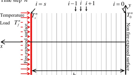
Fig. 1. Node indexing scheme for the one dimensional problem of a section exposed to a fire on one side.

2.1. The Finite Difference Method

The finite difference method is a numerical technique which can be applied to solve partial differential equations. The finite difference approximations of derivatives convert differential equations to algebraic equations. The approximations use uniform grids for each coordinate, including time, as illustrated in Fig. 1. As a convenient shorthand notation, n

i

T represents the temperature at location x i x at t n t: so i is the index for location whereas n is the index for time. If the forward-difference approximation is used in Eq. (1), the finite-difference equation is represented as

 

1

1 1

2

2

n n n n n

p

i i i s i i

T T T T T

k t

x

 

    _ 



 (3)

The finite difference form of the boundary condition at is, Eq. (2), can be expressed as







   



1 n n

n n n n n

s s

f s f s

T T

k q h T T T T

x 





    

 (4)

However, due to the intervals of x in the FDM, the effect of the heat capacity of the system next to the boundary must be included in Eq. (4) [17] as

1

1/ 2 1

2

n n n n

n s s s s

p

T T xT T

q k s

x  t



 _   _  

  (5)

Note that to achieve symmetry in Eq. (5), n

q in Eq. (4) is replaced by qn1/ 2 of Eq. (6). Eq. (5) is rearranged in Eq. (7). Therefore, n 1

s

T  can be solved based on temperature of the previous step.









  



1/ 2 1/ 2 1/ 2

n n n n n

f s f s

q h T  T  T   T (6)

1 2 1/ 2 1

n n

n n s s n

s s

p

T T

t

T q k T

s x x



 _    _   _

 

 _  _ (7)

Temperature

Load T_fn

b

i i1

1

i _y

x

N

o

n

f

ir

e

-e

x

p

o

se

d

su

rf

ac

e

0

n

T

n s

T

0

i

is

Time step n

F

ir

e

-e

x

p

o

se

d

s

u

rf

ac

To avoid violating the second law of thermodynamics in Eq. (3), the stability condition









/ _p / 0.5

k s  t x  has to be satisfied: for finer spatial resolution also smaller time steps are necessary, and the computational cost increases rapidly with spatial resolution. Furthermore, for increasing functions T_f , the value of Tsn1

 _{must be larger than the value of} n s

T . As a result, another stability condition has to be satisfied:

1/ 2 1 ₀

n n n Ts Ts

q k

x

 _   _

 (8)

To compute the temperature profiles, a matrix of the temperatures of all nodal points is computed at each time step. x and t must be manipulated to satisfy the stability conditions during the numerical solution.

2.2. Energy Based Temperature Profile Method, EBM

To simplify the FDM of the 1D analysis, the energy conservation principle and a pre-determined shape function of the temperature profile was adopted by Panedpojaman [16]. The amount of energy transfer to a section under fire exposure, 1

n T

Q , can be approximated as in Eq. (9) [18]. By using the equation, effects of various convection and radiation heat transfers are included in the computation. The amount of heat energy in that section, 1

n I

Q , is computed taking into account the heat capacity of the system, and the temperature profile as shown in Fig. 2. 1

n I

Q can be approximated as in Eq. (10). Based on the energy conservation principle, the cumulative energy transfer 1

n T

Q equals the accumulated heat energy Q_In₁ as in Eq. (11)

 

1

0 0

n

t n

n m

T

m

Q qAdt A q t













1 0

( )

b

n n

I p r

Q 



 





1 1

1 ₀

or ( )

b n

n n m n

T I p r

m

Q Q A q t s A T x T dx









where Tr is the room temperature; A is the surface area; and ( ) n

T x is the temperature profile within the cross section. Assuming uniform temperature of the fire-exposed surface, the surface area can be replaced with unit area (i.e., A1). Furthermore, to improve accuracy of Q_Tn₁, _qn _{is derived in this study based on} an average temperature between n and n1 steps since the temperature is not constant.









 





n n n n n

f s f s

DOI:10.4186/ej.2015.19.2.109

Fig. 2. Heat energy in the section: (a) Low energy case; (b) High energy case. Through the energy conservation principle, n 1

s

T  in Eq. (7) and the temperature in the section can be solved when the shape function of _Tn( )_{x is pre-determined. This study also postulates the shape function}

to be a power function as in Eq. (13). This is suitable for monotonically increasing fire curves. The temperature is always maximum at the fire exposed surface and decreases inwards within the section.

0

( )

n n n

T x C x T (13)

where





 

n n n n

s

C T T b

 

  (14)

 is the power of the function; n

b is the effective depth in which the temperature is higher than the room temperature as described in Fig. 2; and 0

n

T is the temperature at bn.

Two cases of temperature profile are shown in Fig. 2: the low energy case in which 0 n

r T T and n

b  b. bn can be computed through the energy conservation Eq. (11).









1 1

n T n

n p s r Q

b

s T T

 

  

 (15)

the high energy case in which 0 n

r

T T and _bn _b. 0

n

T can also be computed through the energy conservation Eq. (11).





0

1

1

n

n T n

r s r

p Q

T T T T

s b 

 

   

   _  _ 

 _{ } 

  (16)

By substituting the term





n n

s s

T T x with the derivative from Eq. (13) at xbn  x/ 2, Tsn 1

 _in

Eq. (7) and the stability condition (8) can be rewritten as (17) and (18):





1 2 1/ 2 _{/ 2}

n n n n n n n

s s s

p t

T q k C b x T T

s x



 



 _    _  _{ } _{ }

 

   (17)





1/ 2

/ 2 0

n n n n

q k C b x



 

 _ _{  }

(18) The difference between n

f

T and T_sn depends on the time, it is not constant. When the difference is small, the value of _qn1/ 2 _{in Eq. (5) may not satisfy Eq. (18). This condition could occur at any time step in both} typical FDM and the proposed method. Once the dissatisfaction occurs, n1

s

T  is lower than n s

T . By using

y

x

y

x

n

b b

n

b

( )

n

T x

( )

n

T x

Time step n

Time step n

n s

T

0

n r

T T

n s

T

0

n r

T T

1

n T

Q

1

n T

Q

n I

Q

n I

Q

(a)

the FDM, t and x must be re-sized to satisfy the stability condition. However, to simplify the calculation, this study assumes n1 n

s s

T  T at a dissatisfied step n1. Note that, as an increasing function,

the pre-determined shape function cannot violate the second law of thermodynamics within the sections exposed to a monotonically increasing function of fire curves. The stability condition









/ / 0.5

k c  t x  is redundant and is omitted in the EBM.

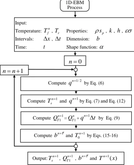
When the value of  is pre-determined, the temperature profiles of sections exposed to a fire can be solved. By using the EBM, the large matrix system of regular FDM can be avoided. The procedure to predict the temperature profile is summarized in Fig. 3.

Fig. 3. Procedure to predict the one-dimensional temperature profiles in a section at step n. 3. Simplified 2D Heat Transfer Analysis

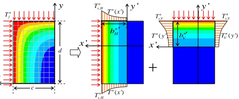
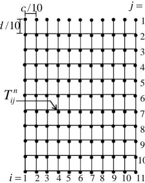
Consider a cross section with dimension of 2d2c exposed to a uniform fire on its four sides. Due to symmetry of the cross section, the analysis involves only a quarter of the section exposed to a fire in two directions as shown in Fig. 4. The decomposition shown in Fig. 4 is applied to approximate the two dimensional problem as a superposition of two one-dimensional problems. The temperature profile and the effective depth, n

b , in each direction are computed by using the 1D procedure in Fig. 3. The subscripts V and Hrepresent the vertical and horizontal direction, respectively.

0

n

1

n n

Output:T_sn1, Q_Tn₁1 , bn1and Tn1( )x

Compute qn1/ 2 by Eq. (6)

Compute T_sn1 and qn1by Eq. (7) and Eq. (12) Compute Q_Tn₁1=Q_Tn₁+qn1t by Eq. (9)

1D-EBM Process

Input:

Temperature: T_fn, T_r Properties: s_p, k, h,  Intervals: x, t Dimension: b

Time: t Shape function: 

DOI:10.4186/ej.2015.19.2.109

Fig. 4. Quarter of a section exposed to fire in two directions and its decomposition model.

Fig. 5. Temperature profiles: (a) overall temperature profile and (b) temperature profile in Zone D. The overall temperature profile is divided into four zones as shown in Fig. 5(a), labeled with A, B, C and D. Zone A is out of the effective area of the heat transfer analysis for both horizontal and vertical analysis. The temperature in this zone, the inner temperature n

i

T , is a constant. T_in is the minimum temperature of the section. Zone B is only in the effective area of the horizontal analysis. The temperature profile in this zone, T_Hn( ')x , varies directly with x', independent of y'. Conversely, Zone C is in the

effective area of the vertical analysis. The temperature profile in Zone C, n( ')

V

T y , varies directly with y'

but is independent of x'.

In Zone D, both horizontal and vertical heat transfer affects. The temperature profile in this zone varies with both x' and y'. Non-homogeneous boundary conditions are given by T_Hn( ')x , T_Vn( ')y ,

( ')

n CH

T x and T_CVn ( ')y , as shown in Fig. 5(a) and Fig. 5(b). The T_CHn ( ')x and T_CVn ( ')y are the surface temperatures in the horizontal and vertical direction of the corner. Note that all functions are based on the trial function in Eq. (13). The continuity conditions are T_CVn (b_Vn)T_CHn (b_Hn)T_Cn, T_CHn (0)T_{s V}n_, ,

,

(0)

n n

CV s H

T T and T_Vn(0)T_Hn(0)T_in. As a result, T_Hn( ')x , T_Vn( ')y , T_CHn ( ')x and T_CVn ( ')y can be described as follows:



AUG 30 2012

21:54:00

NODAL SOLUTION STEP=2 SUB =6300 TIME=14400 TEMP (AVG) RSYS=0 SMN =274.265 SMX =1153

1 2 3 4 5 6 7 8 9 10 11 12 13 14 15 16 17 18 19 20 21 S1 S4 S7 S10 0.60 -0. 80 0.40 -0. 60 0.20 -0. 40 0.00 -0. 20

1

MN

MX

X

Y

Z

22.907

136.922

250.937

364.951

478.966

592.981

706.995

821.01

935.025

1049

11:27:59

AUG 31 2012

NODAL SOLUTION

STEP=1

SUB =120

TIME=7200

TEMP (AVG)

RSYS=0

SMN =22.907

SMX =1049

1

MN

MX

X

Y

Z

22.907

_136.922

250.937

_364.951

478.966

_592.981

706.995

_821.01

935.025

₁₀₄₉

AUG 31 2012

11:27:59

NODAL SOLUTION

STEP=1

SUB =120

TIME=7200

TEMP (AVG)

RSYS=0

SMN =22.907

SMX =1049

n H

b



V b  ( ') n T x ( ') n

T y n( ')

V T y , n s H T , n s V T , n s V T , n s H

T ( ')

n T x d c n f T

'

x

'

y

'

x

'

y

x

y

'

x

B A ( ') n CH T x n C T , (0) n n

CV s H

T T

,

(0)

n n

CH s V

T T

n C T n C T n i T n i T n i T n H b  ( ') n CV T y

( 1', 1')

n

T x y

n i T ( ') n H T x ( 1') n H T x ( 1') n V T y ( ') n V T y , n s V T , n s H T , n s H T n C T ( 1') n CH T x ( 1') n CV T y , n s H T , n s V T (0) n H T  (0) n n V i

T T









( ') '/

n n n n n

H s H i H i

T x T T x b T

 

   (19)









( ') '/

n n n n n

V s v i V i

T y T T y b T

 

   (20)









( ') '/

n n n n n

CH C s V H s V

T x T T x b T

 

   (21)









( ') '/

n n n n n

CV C s H V s H

T y T T y b T

 

   (22)

Based on the overall character of Zone A to Zone C in Fig. 5(a) and the temperature profile in Zone D as shown in Fig. 5(b), the temperature function in the overall section is approximated by













( , )

n n n n n n n n n n

C s H s V i _{n n} s H i _n s V i _n i

H V H V

x y x y

T x y T T T T T T T T T

b b b b

  

 _{ }   _   _ 

     

        

 

   _  _  

    (23)

max( n , 0)

H

x  xb  c (24)

max( _Vn , 0)

y  xb d (25)

The overall temperature profile in Eq. (23) is controlled by six key variables, i.e. n V b , n

H b , n_,

s V T , n_,

s H T , T_Cn and n

i

T . Through the horizontal and vertical analysis of the 1D procedure in Fig. 3, the values of b_Vn, b_Hn, ,

n s V

T and T_{s H}n_, can be computed.

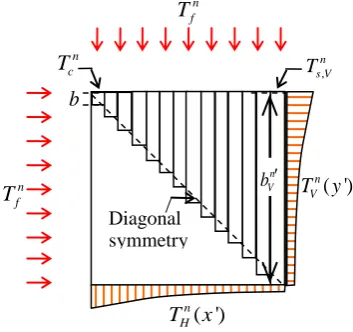
Consider a diagonally symmetric temperature in the corner section, as shown in Fig. 6. The EBM can also be applied to such symmetric cases. The n

C

T is computed by using Eq. (17) in which the analyzed thickness, b, is assumed to be a small value, that is b x.

Fig. 6. Diagonally symmetric temperature.

Based on the decomposition model in Fig. 4, the 2D heat transfer energy of the quarter section with a unit length, 2

n T

Q , is approximated in Eq. (26) and Eq. (27). To evaluate the heat energy in the section exposed to a fire in two directions, 2

n I

Q , Eq. (10) can be rewritten to correspond with the 2D temperature profile in Eq. (28). As a result, n

i

T can be derived, as done in Eq. (29), from the energy conservation principle,

2 2

n n

T I

Q Q (26)

2 1, 1,

n n n

T T H T V

Q cQ dQ (27)





2 0 0

( , )

d c

n n

I p r

Q 

 

n f T

b

Diagonal symmetry

n f T

n c

T n_,

s V

T

n V

b n_{( ')} V T y

( ')

DOI:10.4186/ej.2015.19.2.109









2 , , 1 , 2 , 3

1 2 3

/

n n n n n n

T p r C s H s V s H s V

n i

Q s T cd T T T T T

T

cd

   

  

     



   (29)

where





1 / 1

n n H V b b

     (30)





2 / 1

n H b d

    (31)





2 / 1

n V b c

    (32)

Note that, for the low energy case in which n H

b  c and b_Vn d, b_Hnb_Vn and n_, n_, s H s V T T , the temperature profile does not depend on the section dimension. The procedure to predict the 2D temperature profile is summarized as illustrated in Fig. 7. The EBM is considered as a spreadsheet calculation procedure.

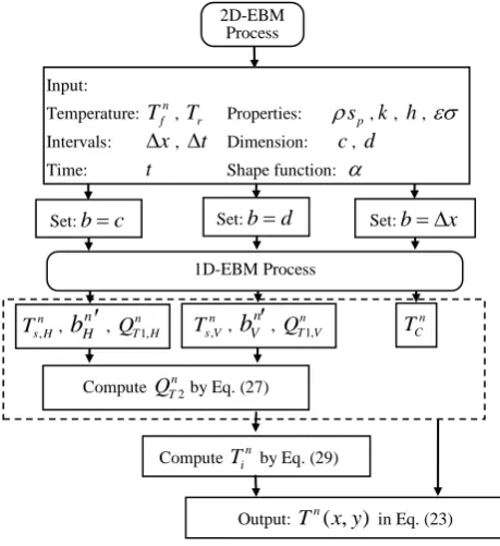
Fig. 7. Procedure to predict the 2D temperature profile.

4. Investigation of Suitable Exponent for the Temperature Profile

Rectangular sections with normal concrete properties are considered in the study. To investigate suitable values of the exponent , the temperature profiles in concrete sections computed by FEM, using ANSYS software, are compared with the proposed method using different exponents. The concrete sections in the comparison are exposed to the nominal temperature-time curves of BSEB 1992-1-2:2004 [1] on their four sides. All the nominal temperature-time curves are monotonically increasing. Due to symmetry, only one quarter of the section exposed to fire on two sides needs to be solved as shown in Fig. 4. The nominal temperature-time curves include the standard temperature-time curve (ST), the external fire curve (EX) and the hydrocarbon curve (HY), shown in Fig. 8. The curve can represent various fire loads which may occur. This study investigates 6 different sizes in this study: 300 mm  300 mm (2c2d), 300mm  600 mm, 400mm  400 mm, 500mm  800 mm, 600mm  600 mm, and 800mm  800 mm. The temperatures for 8 different fire durations, which are 30, 60, 90, 120, 150, 180, 210 and 240 minutes, are scoped in the comparison. The maximum fire resistance in codes is normally 240 minutes. As a result, there are 144 (3x6x8) data sets in the comparison.

2D-EBM Process

n C

T

Input:

Temperature: T_fn, T_r Properties: s_p,k, h,  Intervals: x, t Dimension: c, d

Time: t Shape function: 

Set:bc Set:bd Set:b x

1D-EBM Process

Compute Q_Tn₂by Eq. (27)

Compute T_in by Eq. (29)

Output: _Tn( , )_{x y}

in Eq. (23)

,

n s H

T , b_Hn, Q_{T H}n_1, n_, s V

Fig. 8. Nominal temperature-time curves of BSEB 1992-1-2:2004 [1].

The thermal properties of concrete in accordance with BS EN 1991-1-2 (2002) [19] and BS EN 1992-1-2 (2004) [1] are specified in the computation. The variations of the thermal conductivity k and the product of the density and the specific heat sp with temperature are described in Fig. 9.

2

1.36 0.136( / 100) 0.0057( / 100)

k  T  T W/m Ko (33)

The specific heat capacity with moisture content of 1.5% is applied in the FEM analysis. The thermal conductivity used is a lower bound for concrete, which gives realistic temperatures for concrete structures [1]. The FEM analysis is conducted with variation of the thermal properties with temperatures. To simplify the computation of the EBM, the value of sp is assumed to be constant at 2,300

3 3o

10 J/m K

 , about the

average value of sp in Fig. 9. However, the thermal conductivity k given in Eq. (33) is still used in the EBM. The coefficient of heat transfer-convection h is of 25 W/m2_{°K for the standard temperature-time} and external fire curves and 50 W/m2_{°K for the hydrocarbon curve. Stefan Boltzmann constant and the} resultant emissivity related to the concrete surface are 5.67 x 10-8 _W/m2_°K4 _{and 0.7, respectively.}

To analyze the temperature profile in the section by ANSYS [10], the sections are modeled with three-dimensional solid elements, Solid70, having eight nodes with a single degree of freedom (i.e., temperature) at each node. The surface element, Surf152, is used to account for heat convection and radiation of the fire temperature. The element size of c/ 20d/ 20 is specified for the FEM model whereas x of 10 mm is specified for the EBM analysis. The time increment t of 60 s is used in both methods.

Fig. 9. Thermal properties of concrete.

0 200 400 600 800 1000 1200

0 60 120 180 240

Series1

Series2

Series3

Time (min)

T

em

peratu

re

(

oC

)

HY

ST

EX

(10 W/m K)

k

,

k



s

0 500 1000 1500 2000 2500 3000 3500

0 200 400 600 800 1000 1200

k for FEM and EBM

CD

o

DOI:10.4186/ej.2015.19.2.109

Fig. 10. Nodal points for the error investigation.

The temperatures obtained from the FEM and the EBM with different  values are recorded for the 121 nodal points shown in Fig. 10. An error between the nodal temperatures obtained from the EBM,

, n EBM ij

T , and the nodal temperatures obtained from the FEM, n _, FEM ij

T , is characterized by the normalized absolute error:





, ,

,

max

n n

EBM ij FEM ij n

ij _n

FEM ij

T T

T

   (34)

The variation of the average normalized absolute error, av, with  value is described in Fig. 11. av is the average value of n

ij

 throughout all 144 data sets which is normally 17,424 (121x144) nodal temperatures. However, the data sets with av larger than 0.10 are not included in the averaging, because the EBM is not an appropriate approximation in those cases. The value = 2.6 minimizes av and is optimal in this test panel, as illustrated in Fig. 11.

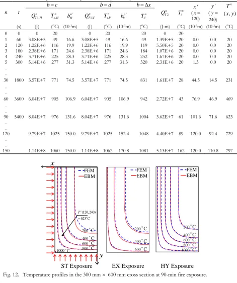
A computational example of the temperature profiles of a 300 mm  600 mm concrete cross section by using the EBM spreadsheet calculation under the ST fire curve is shown in Table 1 for the one dimensional heat transfer and Table 2 for the two dimensional heat transfer. The input parameters used in the table are Tr = 20

o

C,  = 2.6, t = 60 s, x= 10 mm, s_p = 2,30010 J/m K3 3o , k based on the equation in BS EN 1992-1-2 (2004) [1] given in Eq. (33), h = 25 W/m2_°K,  _{= 0.7}_{5.67 x 10}-8 W/m2_°K4_{, c = 150 mm and d = 300 mm. The computation process follows Fig. 3 and Fig. 7. The} temperature profiles from the FEM and the EBM for the section at 90-min fire exposure, is shown in Fig. 12. The figure also depicts the temperature profile of the section under the EX and HY fires.

The approximate solutions are comparatively accurate near the fire exposed surface, giving results very similar to the FEM, but the accuracy diminishes inwards. Another illustration of the accuracy of the EBM is in Fig. 13 and Fig. 14, showing the variation of the temperature distribution along the diagonal line with duration of fire exposure.

Even though the  value of 2.6 provides the minimum av, large values of av (av 0.05) and significantly overestimated heat energy ( 2, / 2, 1.10

n n

T EBM T FEM

Q Q  ) are still typical of the EBM for small size sections with long fire durations, as shown in Fig. 13. 2,

n T EBM

Q is the accumulated heat energy according to the EBM, and 2,

n T FEM

Q is similar according to the FEM. In such cases, the heat transfer energy is high compared with the heat capacity of the sections. T_in /T_cn can be used to indicate the local variation in heat energy of each section. For example, under the same amount of heat transfer energy, n

i

T of a small sized section is higher than that of larger section, due to lower heat capacity. As a result, under the same amount of heat transfer energy, T_in /T_cn is higher in smaller size sections.

1

2

3

4

5

6

7

8

9

10

11

S1

S3

S5

S7

S9

S1

1

0.

8-1

0.

6-0.

8

0.

4-0.

6

0.

2-0.

4

0-0.

2

/10 c

/10 d

i1 2 3 4 5 6 7 8 9 10 11

j

1 2 3 4 5 6 7 8 9 10

Fig. 11. Variation of the average error with  value.

Table 1. 1D computational example of the temperature profiles. n t Tfn

bc 1/ 2

n

q  qn 1,

n T H

Q ₀n

T kn ,

n s H

T n'

H b

(s) (°C) (W/m2_{) (W/m}2_{) (J) (°C)} (W/m°

K) (°C) (10-3m)

0 0 1 0 20 1.33 20

1 60 349 5.56E+3 5.14E+3 3.08E+5 20 1.29 49 16.6 2 120 445 5.56E+3 1.52E+4 1.22E+6 20 1.21 116 19.9 3 180 502 2.03E+4 1.94E+4 2.38E+6 20 1.14 171 24.6 4 240 544 2.32E+4 2.21E+4 3.71E+6 20 1.08 225 28.3 5 300 576 2.50E+4 2.38E+4 5.14E+6 20 1.03 277 31.3

. .

30 1800 842 1.68E+4 1.61E+4 3.57E+7 20 0.65 771 74.5 .

.

60 3600 945 1.25E+4 1.21E+4 6.04E+7 20 0.60 905 106.9 .

.

90 5400 1006 1.06E+4 1.03E+4 8.04E+7 20 0.58 976 131.6 .

.

120 7200 1049 9.52E+3 9.28E+3 9.79E+7 26 0.56 1025 150.0 .

.

150 9000 1082 9.20E+3 9.01E+3 1.14E+8 79 0.56 1060 150.0 The variations of av and 2, / 2,

n n

T EBM T FEM

Q Q with T_in /T_cn are shown in Fig. 15(a) and 15(b), respectively. The figures show that the temperature accuracy of the EBM relates to the accuracy of the energy. Large values of av are found in the cases with significantly overestimated heat energy. The assumption that the decomposition to one dimensional models is a good approximation to 2

n T

Q in Eq. (23), no longer holds. Note that underestimated heat energy for low T_in /T_cn is shown in Fig 15(b), and they normally occur at the early times of fire exposure. The cumulative heat energy is low, and the magnitude of error in the energy is small giving also accurate estimates of the temperature. Fig. 15 suggests that the data sets with T_in /T_cn0.20 (109 data sets) provides accurate cases, with _av 0.05, as summarized in Table

3. In the case of T_in 0.2T_cn, the approximate temperatures are significantly overestimated in the inner area



av



0.00 0.01 0.02 0.03 0.04 0.05

1.5 2 2.5 3 3.5

Series1 0.0213

DOI:10.4186/ej.2015.19.2.109

as shown in Fig. 13. However, the approximate temperatures are still close to the FEM analysis near the surface exposed to fire.

For rectangular concrete sections under various fire exposures, the method mostly provides the conservative temperature prediction. Generally, the method can be used to approximately predict temperature profile, including the 500 o

C isotherm, as well as the temperature of the reinforcing steel

which locates at the near surface.

Table 2. 2D computational example of the temperature profiles.

n t

bc bd b x

2 n T

Q T_in

'

x

(x=

120)

'

y

(y=

240) n T

( , )x y 1,

n T H

Q T_{s H}n_, n' H

b 1,

n T V

Q T_{s V}n_, n' V

b T_Cn

(s) (J) (°C) (10-3_{m) (J) (°C) (10}-3_{m) (°C) (J-m) (°C) (10}-3_{m) (10}-3_{m) (°C)}

0 0 0 20 0 20 20 0 20

1 60 3.08E+5 49 16.6 3.08E+5 49 16.6 49 1.39E+5 20 0.0 0.0 20

2 120 1.22E+6 116 19.9 1.22E+6 116 19.9 119 5.50E+5 20 0.0 0.0 20

3 180 2.38E+6 171 24.6 2.38E+6 171 24.6 184 1.07E+6 20 0.0 0.0 20

4 240 3.71E+6 225 28.3 3.71E+6 225 28.3 252 1.67E+6 20 0.0 0.0 20

5 300 5.14E+6 277 31.3 5.14E+6 277 31.3 320 2.31E+6 20 1.3 0.0 20

. .

30 1800 3.57E+7 771 74.5 3.57E+7 771 74.5 831 1.61E+7 28 44.5 14.5 231

. .

60 3600 6.04E+7 905 106.9 6.04E+7 905 106.9 942 2.72E+7 43 76.9 46.9 469

. .

90 5400 8.04E+7 976 131.6 8.04E+7 976 131.6 1004 3.62E+7 61 101.6 71.6 623

. .

120 9.79E+7 1025 150.0 9.79E+7 1025 152.4 1048 4.40E+7 89 120.0 92.4 729

. .

150 1.14E+8 1060 150.0 1.14E+8 1062 170.8 1081 5.13E+7 162 120.0 110.8 797

Fig. 12. Temperature profiles in the 300 mm  600 mm cross section at 90-min fire exposure.

FEM EBM

200oC

400oC 600oC

800oC

200oC

400oC 600oC

800oC 1000oC 200oC

400oC

600oC

1000o C

FEM EBM

FEM EBM

ST Exposure EX Exposure HY Exposure

x

y

o

(120, 240) 623 C n T

Fig. 13. Variation of the temperature distribution with fire exposure duration along the diagonals of small size sections. 0 200 400 600 800 1000 1200

0 30 60 90 120 150

Series1 Series2 Series3 Series4 0 120 240 360 480 600 720

0 30 60 90 120 150

Series1 Series2 Series3 Series4 0 200 400 600 800 1000 1200

0 30 60 90 120 150

Series1 Series2 Series3 Series4 0 200 400 600 800 1000 1200

0 30 60 90 120 150

Series1 Series2 Series3 Series4 Series5 Series6 0 120 240 360 480 600 720

0 30 60 90 120 150

Series1 Series2 Series3 Series4 Series5 Series6 0 200 400 600 800 1000 1200

0 30 60 90 120 150

Series1 Series2 Series3 Series4 Series5 Series6 0 200 400 600 800 1000 1200

0 40 80 120 160 200

Series1 Series2 Series3 Series4 Series5 Series6 0 200 400 600 800 1000 1200

0 40 80 120 160 200

Series1 Series2 Series3 Series4 Series5 Series6 0 120 240 360 480 600 720

0 40 80 120 160 200

Series1 Series2 Series3 Series4 Series5 Series6

Section : 300300 Fire : ST

Section : 300300 Fire : EX

Section : 300300 Fire : HY

Section : 300600 Fire : ST

Section : 300600 Fire : EX

Section : 300600 Fire : HY

Section : 400400 Fire : ST

Section : 400400 Fire : EX

Section : 400400 Fire : HY 120 mins 60 mins 120 mins 60 mins 120 mins 60 mins 120 mins 60 mins 180 mins 120 mins 60 mins 180 mins 120 mins 60 mins 180 mins 120 mins 60 mins 180 mins 120 mins 60 mins 180 mins 120 mins 60 mins 180 mins

1200 720 1200

1000 600 1000

800 480 800

600 360 600

400 240 400

200 120 200

0 0 0

0 30 60 90 120 150 0 30 60 90 120 150 0 30 60 90 120 150

1200 720 1200

1000 600 1000

800 480 800

600 360 600

400 240 400

200 120 200

0 0 0

0 30 60 90 120 150 0 30 60 90 120 150 0 30 60 90 120 150

1200 720 1200

1000 600 1000

800 480 800

600 360 600

400 240 400

200 120 200

0 0 0

0 40 80 120 160 200 0 40 80 120 160 200 0 40 80 120 160 200

T em peratu re ( o C ) T em peratu re ( o C ) T em peratu re ( o C ) T em peratu re ( o C ) T em peratu re ( o C ) T em peratu re ( o C ) T em peratu re ( o C ) T em peratu re ( o C ) T em peratu re ( o C )

Horizontal Distance (mm) Horizontal Distance (mm) Horizontal Distance (mm) Horizontal Distance (mm) Horizontal Distance (mm) Horizontal Distance (mm) Horizontal Distance (mm) Horizontal Distance (mm) Horizontal Distance (mm)

FEM EBM

Horizontal Distance (mm) d

c

DOI:10.4186/ej.2015.19.2.109

Fig. 14. Variation of the temperature distribution with fire exposure duration along the diagonals of large size sections.

Fig. 15. Variation of av and 2, / 2,

n n

T EBM T FEM

Q Q with n / n

i c T T . 0 200 400 600 800 1000 1200

0 50 100 150 200 250

Series1 Series2 Series3 Series4 Series5 Series6 Series7 Series8 0 120 240 360 480 600 720

0 50 100 150 200 250

Series1 Series2 Series3 Series4 Series5 Series6 Series7 Series8 0 200 400 600 800 1000 1200

0 50 100 150 200 250

Series1 Series2 Series3 Series4 Series5 Series6 Series7 Series8 0 200 400 600 800 1000 1200

0 60 120 180 240 300

Series1 Series2 Series3 Series4 Series5 Series6 Series7 Series8 0 120 240 360 480 600 720

0 60 120 180 240 300

Series1 Series2 Series3 Series4 Series5 Series6 Series7 Series8 0 200 400 600 800 1000 1200

0 80 160 240 320 400

Series1 Series2 Series3 Series4 Series5 Series6 Series7 Series8 0 120 240 360 480 600 720

0 80 160 240 320 400

Series1 Series2 Series3 Series4 Series5 Series6 Series7 Series8 0 200 400 600 800 1000 1200

0 80 160 240 320 400

Series1 Series2 Series3 Series4 Series5 Series6 Series7 Series8

Section : 500800 Fire : ST

Section : 500800 Fire : EX

Section : 500800 Fire : HY

Section : 600600 Fire : ST

Section : 600600 Fire : EX

Section : 800800 Fire : ST

Section : 800800 Fire : EX

Section : 800800 Fire : HY

180 mins 60 mins 240 mins 120 mins 180 mins 60 mins 240 mins 120 mins 180 mins 60 mins 240 mins 120 mins 0 200 400 600 800 1000 1200

0 60 120 180 240 300

Series1 Series2 Series3 Series4 Series5 Series6 Series7 Series8

Section : 600600 Fire : HY

180 mins 60 mins 240 mins 120 mins 180 mins 60 mins 240 mins 120 mins 180 mins 60 mins 240 mins 120 mins 180 mins 60 mins 240 mins 120 mins 180 mins 60 mins 240 mins 120 mins 180 mins 60 mins 240 mins 120 mins

1200 720 1200

1000 600 1000

800 480 800

600 360 600

400 240 400

200 120 200

0 0 0

0 50 100 150 200 250 0 50 100 150 200 250 0 50 100 150 200 250

1200 720 1200

1000 600 1000

800 480 800

600 360 600

400 240 400

200 120 200

0 0 0

0 60 120 180 240 300 0 60 120 180 240 300 0 60 120 180 240 300

1200 720 1200

1000 600 1000

800 480 800

600 360 600

400 240 400

200 120 200

0 0 0

0 80 160 240 320 400 0 80 160 240 320 400 0 80 160 240 320 400

T em peratu re ( o C ) T em peratu re ( o C ) T em peratu re ( o C ) T em peratu re ( o C ) T em peratu re ( o C ) T em peratu re ( o C ) T em peratu re ( o C ) T em peratu re ( o C ) T em peratu re ( o C )

Horizontal Distance (mm) Horizontal Distance (mm) Horizontal Distance (mm) Horizontal Distance (mm) Horizontal Distance (mm) Horizontal Distance (mm)

Horizontal Distance (mm) Horizontal Distance (mm) Horizontal Distance (mm)

FEM EBM

0.40 0.60 0.80 1.00 1.20 1.40 1.60

0.0 0.2 0.4 0.6 0.8 1.0 1.2

Series1 0.00 0.05 0.10 0.15 0.20 0.25 0.30

0 0.2 0.4 0.6 0.8 1 1.2

Series1

(a) (b)

35 data sets 109 data sets 109 data sets

35 data sets

av



/

n n

T EBM T FEM

Table 3. Accurate cases for the EBM analysis. Section

(mm)

Fire duration (min) for accurate temperature prediction (T_in 0.2T_cn)

ST EX HY

300300 <150 <90 <120

300600 <180 <120 <150 400400 <240 <150 <180

500800 0 to 240

600600 0 to 240

800800 0 to 240

5. Comparing with Experimental Temperature

The EBM is validated by comparing the predicted temperature with the data of experiments and the FEM analysis. The experimental temperatures of RC sections under fire exposure from Lie et al. [20] reported in [13], Jau and Huang [21], Abbasi and Hogg [22], and Dwaikat and Kodur [23] are used in the comparison. Details of the dimensions, the fire load (ASTM E119 [24], BS 476 [25] and ISO 834 [26]) and the location of temperature measurement are described in Fig. 16. The thermal properties are assumed to be in accordance with BS EN 1991-1-2 [19] and BS EN 1992-1-2 [1]. The effects of reinforcing steel in RC sections on the heat transfer analysis are neglected, due to its relatively small area [8]. Points D and E are at the reinforcing locations.

The comparisons of the experimental temperature–fire duration relationship at the measured points and the temperature profiles with those of the EBM and the FEM are shown in Fig. 17 and Fig. 18, respectively. Note that, to limit the influence zone of unexpected fire [21], the temperature profile in Fig. 18 is described in the dimension of 250mm  300 mm. As shown in Fig. 17, the EBM temperatures are slightly low at early times, compared with both experimental results and FEM analysis. Latterly, the EBM temperatures move closely to the other methods. A good agreement between the EBM and the other methods is observed. Even though the FEM analysis includes non-constant thermal properties, the simplified EBM approximation still delivers closely similar results.

Fig. 16. Details of the experiments and the locations of temperature measurement: (a) Lie et al. [20], (b) Jau and Huang [21], (c) Abbasi and Hogg [22], and Dwaikat and Kodur [23].

25 64

152

A B C

Dimension in mm

Column 305305

ASTM E-119 4-sided fire exposure

Beam 300400

75 60 D

BS 476 / ISO 834 3-sided fire exposure

Column 300450

BS 476 / ISO 834 2-sided fire exposure

64 54

Beam 254406

102

102 127

E G

F

ASTM E-119 3-sided fire exposure

DOI:10.4186/ej.2015.19.2.109

Fig. 17. Comparison of experimental temperature–fire duration relationship at the measured points with the EBM and the FEM: (a) the experiment of Lie et al. [20], (b) the experiment of Abbasi and Hogg [22], and (c) the experiment of Dwaikat and Kodur [23].

Fig. 18. Comparison of experimental temperature profiles from Jau and Huang [21] with the EBM and the FEM.

0

200

400

600

800

1000

1200

0

30

60

90

120

25

64

152

1200

1000

800

600

400

200

0

Fire duration (minutes)

ASTM-E119

A

B

C FEM EBM Test [20]

T

em

p

er

atu

re

(

o C

)

0 30 60 90 120

(a)

Fire duration (minutes)

T

em

p

er

atu

re

(

o C

) ASTM-E119

(c)

FEM EBM Test [23]

E

F G

0 200 400 600 800 1000 1200

0 30 60 90 120

Se rie s1 Se rie s2 Se rie s3 Se rie s4 Se rie s5 Se rie s6 0

200 400 600 800 1000 1200

0 30 60 90 120 150

D

Fire duration (minutes)

T

em

p

er

atu

re

(

o C

) BS 476 / ISO 834

(b)

FEM EBM Test [22]

120 minutes _{240 minutes}

3

0

0

m

m

250 mm

FEM EBM Test [21]

200oC

400oC

600oC 800oC

1000oC

200oC

400oC

600oC

800oC

6. Conclusion

In this study, an energy based method is firstly developed to predict temperature profiles in rectangular concrete section. An energy based method for heat transfer analysis is developed based on the energy conservation principle and a pre-determined power function for temperature profiles in concrete sections with the simplified normal properties. The power function is suitable for monotonically increasing fire curves. According to the energy conservation principle, the cumulative heat energy transferred from the boundary equals the heat energy accumulated within a fire-exposed section. The heat energy within the section is computed based on the heat capacity and the temperature profile. As a result, the temperature function in the section can be computed.

The heat transfer energy of a rectangular section exposed to fire from two directions is evaluated based on decomposition to superposed one dimensional models, in which the energy can be computed by one-dimensional heat transfer analysis. Through the energy conservation principle, the temperature function in the overall section is evaluated. The temperature profile of a rectangular section is controlled by six key variables that are the horizontal and vertical surface temperature, the horizontal and vertical effective depth, the corner temperature, and the inner temperature.

On comparing the EBM approximation with the FEM computations for various concrete sections and fire loads, the exponent = 2.6 minimizes the average error. However, the EBM approximation significantly overestimates the energy if the predicted minimum temperature exceeds 0.2 times the predicted maximum temperature. In such cases, the decomposition to one dimensional problems is a poor approximation. This characterizes the limitation of the EBM approximation in some cases. However, for normal use, the EBM is validated by comparing the predicted temperature with the experimental and FEM results. Even though the FEM analysis includes non-constant thermal properties, the simplified EBM approximation still delivers closely similar results.

7. Discussion

The proposed method can be used to predict the temperature profile in rectangular section, such as beams and columns, with normal concrete properties. The method suitable for the section under various fire loads in two directions and can be implemented as a spreadsheet calculation. Design engineers can apply the EBM approximation as an alternative method to evaluate the temperature profile in a regular spreadsheet program. The proposed method facilitates analysis of heat transfer, necessary to ensure fire resistance of concrete structures under various fire scenarios. By using the EBM approximation, the complications of using FEM or FDM can be avoided. However, the proposed method is limited to rectangular concrete section under monotonically increasing fire curves and the predicted minimum temperature less than 0.2 times the predicted maximum temperature. For cases exceeding the limitations, using FEM or FDM is required. Further developments on the EBM approximation may overcome such limitations.

Acknowledgement

This research was financially supported by Faculty of Engineering, Prince of Songkla University, contract no. ENG-55-2-7-02-0139-S. We would like to sincerely thank the copy-editing service of Research and Develop Office and Assoc. Prof. Dr. Seppo Karrila who dedicated their time to provide valuable comments.These supports are gratefully acknowledged

References

[1] BSI, “Eurocode 2: design of concrete structures– Part 1–2: general rules- structural fire design,” BS EN1992-1-2, British Standards Institution, London, 2004.

[2] T. Pothisiri and N. Hemathulin, “Test data on intumescent fire protection for structural steel sections in Thailand,” Engineering Journal, vol. 16, no. 2, pp. 85–92, 2012.

[3] ACI, “Standard Method for Determining Fire Resistance of Concrete and Masonry Construction Assemblies,” ACI Committee 216.1, American Concrete Institute, Detroit, 2007.

[4] A. Haji-Sheikh and J. V. Beck, “Temperature solution in multi-dimensional multilayered bodies,” Int. J.

DOI:10.4186/ej.2015.19.2.109

[5] F. de Monte, “Unsteady heat conduction in two-dimensional two slab-shaped regions. Exact closed-form solution and results,” Int. J. Heat Mass Transfer, vol. 46, pp. 1455–1469, 2003.

[6] D. Di Capua and A.R. Mari, “Nonlinear analysis of reinforced concrete cross-sections exposed to fire,” Fire Saf. J., vol. 42, pp. 139–149, 2007.

[7] Z. H. Wang and K. H. Tan, “Temperature prediction of concrete-filled rectangular hollow sections in fire using Green’s function method,” J. Eng. Mech., vol. 133, pp. 688–700, 2007.

[8] T. T. Lie, Structural Fire Protection, ASCE Manuals and Reports of Engineering Practice, No. 78, American Society of Civil Engineers, New York, 1992.

[9] J. M. Franssen, V. K. R. Kodur, and J. Mason, User’s Manual for SAFIR 2004, A Computer Program for Analysis of Structures Subjected to Fire, University of Liege, Liege, 2005.

[10] ANSYS, ANSYS multiphysics. Version 11.0 SP1, ANSYS Inc., Canonsburg (PA), 2007.

[11] E. Chowdhury, L. Bisby, and M. Green, “Heat transfer and structural response modelling of FRP confined rectangular concrete columns in fire,” Constr. Build. Mater., vol. 32, pp. 77–89, 2012.

[12] K. S. Chung, S. Park, and S. M. Choi, “Material effect for predicting the fire resistance of concrete-filled square steel tube column under constant axial load,” J. Constr. Steel Res., vol. 64, pp. 1505–1515, 2008.

[13] S. F. El-Fitiany and M. A. Youssef, “Assessing the flexural and axial behaviour of reinforced concrete members at elevated temperatures using sectional analysis,” Fire Saf. J., vol. 44, pp. 691–703, 2009. [14] U. Wickstrom, “A very simple method for estimating temperature in fire exposed concrete structures,”

Fire Technology Technical Report SP-RAPP 1986, Swedish National Testing Institute, pp. 186–194, 1986.

[15] A. H. Buchanan, Structural Design for Fire Safety, John Wiley & Sons Ltd, 2002.

[16] P. Panedpojaman, “Energy based temperature profile for heat transfer analysis of concrete section exposed to fire on one side,” World Academy of Science, Engineering and Technology, vol. 6, no. 5, pp. 853– 858, 2012.

[17] K. V. Wong, Intermediate Heat Transfer. New York: Marcel Dekker, INC., 2003.

[18] V. K. R. Kodur, P. Pakala, and M. B. Dwaikat, “Energy based time equivalent approach for evaluating fire resistance of reinforced concrete beams,” Fire Saf. J., vol. 45, pp. 211–220, 2010.

[19] BSI, “Eurocode 1: actions on structures – Part 1–2: general actions – actions on structures exposed to fire,” BS EN 1991-1-2, British Standards Institution, London, 2002.

[20] T. T. Lie, T. D. Lin, D. E. Allen, and M. S. Abrams, “Fire resistance of reinforced concrete columns,” Technical Paper No. 378, Division of Building Research, National Research Council of Canada, Ottawa, ON, Canada, 1984.

[21] W. C. Jau and K. L. Huang , “A study of reinforced concrete corner columns after fire,” J. Cem. Concr.

compos., vol. 30, pp. 622–638, 2008.

[22] A. Abbasi and P. J. Hogg, “Fire testing of concrete beams with fibre reinforced plastic rebar,” Compos.:

Part A, vol. 37, pp. 1142–1150, 2006.

[23] M. B. Dwaikat, and V. K. R. Kodur, “Response of Restrained Concrete Beams under Design Fire Exposure,” J. Struct. Eng., vol. 135, pp. 1408-1417, 2009.

[24] ASTM, “Standard test methods for fire tests of building construction and materials,” ASTM E119-2007, American Society for Testing and Materials, 2007.

[25] BS, “Fire tests on building materials and structures—Part 20: method from determination of the fire resistance of elements of construction (general principles),” BS 476-3:1987, BSi, UK, 1987