This is a repository copy of
Ab initio formulation of the four-point conductance of
interacting electronic systems
.
White Rose Research Online URL for this paper:
http://eprints.whiterose.ac.uk/4032/
Article:
Bokes, P., Jung, J. and Godby, R. W. orcid.org/0000-0002-1012-4176 (2007) Ab initio
formulation of the four-point conductance of interacting electronic systems. Physical
Review B. 125433. -. ISSN 2469-9969
https://doi.org/10.1103/PhysRevB.76.125433
[email protected] https://eprints.whiterose.ac.uk/ Reuse
Items deposited in White Rose Research Online are protected by copyright, with all rights reserved unless indicated otherwise. They may be downloaded and/or printed for private study, or other acts as permitted by national copyright laws. The publisher or other rights holders may allow further reproduction and re-use of the full text version. This is indicated by the licence information on the White Rose Research Online record for the item.
Takedown
If you consider content in White Rose Research Online to be in breach of UK law, please notify us by
promoting access to White Rose research papers
Universities of Leeds, Sheffield and York
http://eprints.whiterose.ac.uk/
White Rose Research Online URL for this paper:
http://eprints.whiterose.ac.uk/4032
Published paper
Jung, J, Bokes, P, Godby, R.W (2007) Ab-initio formulation of the 4-point
conductance of interacting electronic systems
Physical Review B 76 (125433 - 8 pages)
arXiv:0705.1568v2 [cond-mat.mtrl-sci] 4 Oct 2007
Ab-initio formulation of the 4-point conductance of interacting electronic systems
P. Bokes,1, 2,∗ J. Jung,3, 1 and R. W. Godby1
1Department of Physics, University of York, Heslington, York YO10 5DD, United Kingdom 2Department of Physics, Faculty of Electrical Engineering and Information Technology,
Slovak University of Technology, Ilkoviˇcova 3, 812 19 Bratislava, Slovak Republic
3Physics Division, National Center for Theoretical Sciences, P.O. Box 2-131, Hsinchu, Taiwan (Dated: February 1, 2008)
We derive an expression for the 4-point conductance of a general quantum junction in terms of the density response function. Our formulation allows us to show that the 4-point conductance of an interacting electronic system possessing either a geometrical constriction and/or an opaque barrier becomes identical to the macro-scopically measurable 2-point conductance. Within time-dependent density-functional theory the formulation leads to a direct identification of the functional form of the exchange-correlation kernel that is important for the conductance. We demonstrate the practical implementation of our formula for a metal-vacuum-metal interface.
PACS numbers: 73.63.-b, 71.15.Mb, 73.40.Jn, 05.60.Gg
I. INTRODUCTION
Impressive progress has been achieved within the non-equilibrium Green’s function (NEGF) formulation of quan-tum transport using the simple ground-state density-functional exchange-correlation potential in a self-consistent formula-tion1,2 (NEGF-DFT). However, limitations of the latter ap-proximation were recently identified3,4,5,6,7,8,9,10. For in-stance, NEGF-DFT’s omission of the derivative-discontinuity in the exchange-correlation energy functional was found re-sponsible for serious errors in transport calculation through localized resonant levels5,6. Improvements through an (spin-) unrestricted NEGF-DFT formulation have been argued to describe properly some aspects of the Coulomb blockade in quantum junctions7. At this level of the theory the exchange-correlation potential of the equilibrium system, vxc, is
respon-sible for the electron interaction effects.
In a further theoretical development, Na Sai et al.3 iden-tified a dynamical correction to the resistance of a quantum junction stemming from the contribution of the exchange-correlation electric field to the overall drop in the total po-tential. They estimated the correction within time-dependent current-density functional theory11 (TDCDFT) and showed that it has its origin in the non-local density-dependence of the functional. The very applicability of time-dependent density-functional theory (TDDFT) to the problem of quantum trans-port in the long-time limit has been discussed in depth by Ste-fanucci and Almbladh8and by Di Ventra and Todorov9.
Several authors have proposed alternative treatments that avoid the complexities of the exchange-correlation kernels of TD(C)DFT, either by treating the central region with the configuration integration method12,13while approximating the non-equilibrium distribution of the electrons, or by using the usual NEGF-DFT approach in combination with a model self-energy within the central region14. More systematic approach to the self-energy can be obtained through well tested approx-imations like the GW method15,16. Due to the large computa-tional demand so far only very small systems with restricted size of the basis set could be studied. However, the results are encouraging, e.g. the Kondo effect phenomenology seems to
be well described within the self-consistent GW method16. Nonetheless, a systematic approach for addressing the con-ductance of a fully interacting system at the ab-initio level is not available. This is partly due to the fact that the very formulation of the NEGF formalism17 is based on the con-cept of noninteracting electrodes and demands partitioning of the system and the electron-electron interaction18. Stefanucci and Almbladh8showed that the partitioning can be avoided in principle but practical inclusion of the many-body interactions into the formalism seems to be extremely cumbersome. Fortu-nately, partitioning is not necessary within the linear response formulation. Several authors have addressed the conductance of interacting system of electrons within the framework of the Kubo formalism arriving at a 2-point Landauer-like formula for the conductance10,19,20,21 by making certain assumptions about the steady-state total electric field. There is, however, a problem with this derivation since it ignores the charge re-distribution in the conducting system when the steady state is forming. In fact, ignoring these aspects one quickly arrives at various unphysical corrections to the conductance22. The problem of charge redistributions has been first pointed out by Thouless23. Later Kamenev and Kohn24cast it into a self-consistent framework for many-terminal conductance.
In our work we further develop the formalism that treats the charge redistribution correctly, find its physical interpretation in terms of a time-dependent transient process that leads to the establishment of a current-carrying steady state, and de-rive a closed formula for the 4-point conductance that is well-defined formally as well as physically.
2
one electrode to the other until a certain potential difference between these two is established. For modeling purposes this mechanism cannot be used directly42. Here we will use a construct based on an auxiliary homogeneous vector poten-tial~Aaux(t) =−Rt
0~Eaux(t′)dt′, pointing in the direction of the eventual flow of current, giving a momentum transfer to all the electrons in the infinite system within a finite interval of time. (This auxiliary vector potential is similar in spirit to the one used by R. Gebauer and R. Car to model a nanojunction using periodic boundary conditions26. There, in contrast to our work, the vector potential grows linearly in time for all
t>0 and the work exerted on the system must be dissipated via auxiliary phonons located in the electrodes.) The infinite extent of the system is formally essential to our treatment. It is necessary for a continuous spectrum and for giving a mo-mentum transfer at t=0 to infinitely many electrons present in the system so that the current will flow for all times t>0. However, we would like to mention already at this point that in practical calculations the necessity of the infinite extension can be relaxed so that the formulation can be used for practical
ab-initio calculations.
II. THE NON-LOCAL CONDUCTIVITY AND CONDUCTANCE
The response of the current density to a general external electric field is given within the linear response theory by27
~j(~r,t) =
Z t −∞dt
′Z d3r′~~σ(~r,~r′;t−t′)·~Eext(~r′,t′). (1)
For simplicity we introduce a symbolic notation for the above equation in the form~j=~~σ⋆ ~Eext. In our work, the role of the
external field is taken by the auxiliary field~Eauxthat is homo-geneous and has only a finite duration, i.e. it is absent for large times and it bears no information about the drop in potential in the long-time limit. The latter is contained within the induced field~Ei(~r,t), which appears explicitly when considering the
irreducible (or proper) conductivity28,29,
~j=~~σ⋆ ~Eaux=~~σirr⋆(~Eaux+~Ei). (2)
The induced field accounts for the electron-electron interac-tion at the Hartree level, which is usually referred to as the long-range effects of the Coulomb interaction, whereas the rest of the interactions between electrons, the short range part, is included within the irreducible conductivity. The quantity in which we are primarily interested in is the conductance, defined as G=I/V where V is a voltage drop. For G, the
de-tailed spatial and time dependence of the current density and the induced field while the steady current is being established are of no relevance. We define the voltage drop as the overall drop in potential of the induced field~Eialong the current flow (along the z axis) between far left and far right,
V =lim
t→∞
Z +∞ −∞
dzEzi(~r,t), (3)
00000 00000 00000 00000 00000 00000 00000 00000 00000 00000 00000 00000 00000 00000 00000 00000 00000 00000 00000 00000 00000 00000 00000 00000 00000 00000 00000 00000 00000 00000 00000 00000 11111 11111 11111 11111 11111 11111 11111 11111 11111 11111 11111 11111 11111 11111 11111 11111 11111 11111 11111 11111 11111 11111 11111 11111 11111 11111 11111 11111 11111 11111 11111 11111 00000 00000 00000 00000 00000 00000 00000 00000 00000 00000 00000 00000 00000 00000 00000 00000 00000 00000 00000 00000 00000 00000 00000 00000 00000 00000 00000 00000 00000 00000 00000 00000 00000 00000 00000 00000 11111 11111 11111 11111 11111 11111 11111 11111 11111 11111 11111 11111 11111 11111 11111 11111 11111 11111 11111 11111 11111 11111 11111 11111 11111 11111 11111 11111 11111 11111 11111 11111 11111 11111 11111 11111 j>0 V ∆µ I>0 j=0
FIG. 1: (Color-online) Measurement of the voltage between the macroscopic electrodes, where the current density is zero, gives the two-point conductance G2P=I/(∆µ/e). Measuring the voltage drop inside the simulation box (supercell), where the current density is nonzero, gives the four-point conductance G4P=I/V . Increasing
the supercell the two quantities approach each other (see Sec. V).
which will be indicated by a superscript 4P in the associated 4-point conductance, G4P. This definition is most suitable for ab-initio modeling and does not suffer from ambiguities present when one considers two chemical potentials. In meso-scopic physics, the above definition of conductance is referred to as the 4-point conductance (hence the superscript) since it represents measurement of the voltage drop using contacts different from those acting as a source and drain of the cur-rent. In the extreme case of a 1D conducting channel of non-interacting, but locally neutral electrons it reduces to the well-known expression G4P= (2e2/h)(T/R). This is in contrast with the most frequently encountered 2-point conductance,
G2P, where the voltage drop is understood to be the difference in electro-chemical potentials of the two macroscopic elec-trodes,∆µ/e (see Fig. 1). Since the electrodes are not part of
the quantum-mechanical model of the conducting channel, the familiar Landauer result G2P= (2e2/h)T is believed not to be
derivable from the Kubo formalism30and its plausible deriva-tions are always accompanied with steps motivated by phys-ical insight and arguments about phase-incoherent adiabati-cally widening electrodes31. Here we show that for a nanocon-tact between massive electrodes the 4-point conductance ap-proaches the 2-point Landauer formula. However we never make a reference to∆µ/e and we consistently work with the
drop in the induced electrostatic potential only. Our claims for its applicability for the experimental 2-point conductance fol-low from the fact that for massive electrodes connected with a nanojunction the current density in the electrodes goes to zero and thereby the drop in the induced (Hartree) potential is an excellent indicator of the phenomenological quantity∆µ/e.
[image:4.612.327.554.50.187.2]3
III. SINGULARITY IN THE RESPONSE FUNCTION AND THE 2-POINT CONDUCTANCE
An essential property of the conductivity response function of extended systems capable of coherent transport is their sin-gular long range character for large times or – equivalently – as the frequency approaches zero21. To show this behavior ex-plicitly we need to introduce a few geometrical details of the studied nanojunction which do not restrict the generality of our argument. We consider a geometry where z is a direction of the current flow, q a reciprocal vector in that direction, and for clarity we assume that the system can be put into a peri-odic supercell along the x,y directions. The conductance G4P
is then a conductance for the area of the supercell S. To find the current flowing through S, we integrate Eq. (2) across the cross-sectional area. This naturally leads to the cross-section integrated conductivity32
σirr(z,z′;t) =Z
S
Z
S
d~S·~~σirr(~r,~r′;t)·d~S′, (4) which relates the current to the z-component of the total field,
I(z,t) =
Z t
dt′
Z ∞ −∞
dz′σirr(z,z′;t−t′)(Eaux(t′) +Ei(z′,t′)).
(5) The singular long-range character appears as the indepen-dence ofσirr(z,z′;t)on z and z′ as t→∞which when per-forming the Fourier transforms z,z′→q,q′ and t→ω+iα, takes the form21
lim
ω→0σ
irr(q,q′,ω+iα) =2πG2Pδ(q)δ(q′), (6)
where we have formally introduced the 2-point conductance,
G2P, as the strength of the above mentioned singular character. To extract the strength we introduce a linear functionalGσ[]
Gσ[σirr] = lim
α→0+
Z Z dqdq′ 2π σ
irr(q,q′; iα), (7)
for which we simply have G2P=Gσ[σirr]. It has been shown previously that this identification is correct for noninteracting electrons21. Further motivation to refer to it as a 2-point con-ductance for interacting systems will be discussed in Section V.
IV. ONSET OF THE CURRENT INSIDE THE ELECTRODES
The Eq. (5) can now be analyzed in the light of the above observations. First, let us consider a distant part of one of the electrodes,|z| ≫0, for times such that 1/EF≪t≪ |z|/vF,
where EF and vF are the Fermi energy and Fermi speed
re-spectively. In this regime, the response in the electrodes (|z| ≫0) is determined by the electrode itself, independently of the nanojunction. After a short relaxation time (∼1/EF)
the auxiliary field establishes a uniform (i.e. z-independent) current inside the electrode
I(z,t) =
Z
dz′
Z t
−∞
dt′σirr,e(z,z′;t−t′)Eaux(t′), (8)
whereσirr,e is the irreducible conductivity of the electrode only43while preserving the local charge neutrality within the electrode. We are free to choose any time-dependence of the field as long as it delivers finite change of momentum for each electron and thus establishes the eventual steady current; the most convenient choice is Eaux(t) =−Aauxδ(t), where Aauxis the magnitude of the change in the homogeneous vector po-tential at t=0.
This picture is not valid as one approaches the region of the nanojunction, i.e. for z∼0. Still, since the current will keep coming from the left electrode and disappearing into the right electrode (there is always such|z| ≫0 that for any time
t we have t ≪ |z|/vF and hence the above analysis can be
applied), the charge will have to pile up in front of the junction and similarly deplete behind the junction, creating a resistivity dipole25. The incoming current cannot be decreased by some form of reflected front/disturbance from the junction since this would break the local charge neutrality within the electrode, leading to strong opposing fields. Hence the dipole around the junction and therefore the drop in the induced potential V will grow, increasing the current in the junction region until it becomes equal to the current, I, deep inside the electrode, as described in the preceding paragraph. This will be possible since in the linear regime we expect I=G4PV .
Having in mind this physical process, the established uni-form current at long times expressed by Eq. (8) for the distant electrode applies at all positions including z=0. We express the electrode conductivityσirr,e in reciprocal space for long
times as
I(t→∞) = − lim
α→0+
Z
dqσirr,e(q,q′=0; iα)Aaux (9)
= Fσ[σirr,e]Aaux, (10)
where we use a small imaginary frequency iα to perform the long-time limit27. The linear functionalFσ[]will be further
discussed in Section VII.
V. THE 4-POINT FORMULATION OF THE CONDUCTANCE
The above physical picture can be directly used within Eq. (5). We write the conductivity of the whole system as the conductivity of an infinitely long electrode alone,σirr,e, plus a further term,σirr,j, characterizing the presence of the junction:σirr=σirr,e+σirr,j. Eq. (5) is thereby cast into the
form
I = σirr,e⋆Eaux+σirr,j⋆Eaux+σirr⋆Ei. (11)
Evaluating this equation at z=0 and using the definitions of the functionalsFσ andGσ, the equation (11) can be written
as
I = Fσ[σirr,e]Aaux+Fσ[σirr,j]Aaux+Gσ[σirr]V.(12)
4
third terms sum to zero, from which we easily arrive at the central result of this paper
G4P= F σ[σirr,e]
Fσ[σirr,e]−Fσ[σirr]×G
σ[σirr], (13)
where we have used the fact that Fσ[σirr,j] =Fσ[σirr]− Fσ[σirr,e]and that V=R
dzEi(z) =Ei(q=0).
It is very instructive to apply the above result for a simple 1D non-interacting gas with a single scattering center44. For this system, the noninteracting conductivity in the small fre-quency limit has a form24
σ0(q,q′; iα) = 2
π vFα
v2Fq2+α2δ(q−q ′)
−R2
π vFα
v2
Fq2+α2
2
π
vFα
v2
F(q′)2+α2
(14)
The irreducible conductivity of the homogeneous 1D gas, cor-responding here to the electrode in the general case is simply the first part of the above expression
σ0,e(q,q′; iα) = 2
π vFα
v2
Fq2+α2
δ(q−q′). (15)
It is straightforward to see that using the above forms we haveGσ[σ0] = (1−R)/π =T/π, Fσ[σ0,e]∼v
F/πα and Fσ[σ0,j]∼RvF/πα, and we arrive at the 4-point
conduc-tance G4P= (1/π)(T/R). The arguments of local charge neu-trality in the electrodes and its consequences are very closely related to the original comment by Thouless23and a more re-cent work by Kamenev and Kohn24. In the form presented in Eq. (13) it is valid for nanojunctions of any shape as long as we can put them into a supercell, including the extreme case of a planar metal-vacuum-metal junction for which we will demonstrate its applicability in Section VII.
The generality of Eq. (13) can be used to show the equiva-lence of the 2-point and 4-point conductances for nanojunc-tions with massive electrodes. The demonstration is based on the observation that for such a geometry Fσ[σirr,e]≫ Fσ[σirr] and hence the prefactor containing the F[]s in
Eq. (13) goes to 1. The mentioned inequality is immedi-ately clear from the following argument:Fσ[σirr,e]gives the
current flowing in the electrodes when the vector potential is changed from zero to Aaux, whereasFσ[σirr]formally gives
current as a response to the same disturbance but in a fictitious system having the same geometry as the real nanojunction but for which the long-range Coulomb interaction is missing. This implies that the local charge neutrality is not enforced (since only the irreducible response entersFσ) and as a result most of the electrons coming from one electrode will be reflected from the nanojunction and decrease the current. Hence the re-sulting current will be much smaller in this second case and the inequality is fulfilled. This formally justifies Landauer’s arguments in favor of the expression G=T/πas the conduc-tance of a nanojunction between two phase-randomizing and adiabatically widening reservoirs. As we can clearly see, it is only the widening that is really needed to have the conduc-tance of the junction as a whole be given by Eq. (7). This ex-plains our motivation to refer to the latter quantity as a 2-point
conductance even for interacting electronic systems. The ar-gument applies also to opaque barriers, not necessarily having a constriction, which has been explored in previous works33,34 and is also demonstrated in Section VII.
VI. INCLUSION OF EXCHANGE AND CORRELATION INTO CONDUCTANCE
Having established the validity and generality of Eq. (13) we can proceed to approximations that go beyond non-interacting or Hartree-like non-interacting electrons. The sim-plest way to do so is within the framework of time-dependent density-functional theory. Some doubt about the applicability of the latter might arise from the dynamics deep in the elec-trode described in Section IV. There, the induced current is dominated by a divergenceless component that cannot be re-lated to a time-dependent density, which is the only physically relevant quantity within the TDDFT. However, at the level of Fermi-liquid theory, this divergenceless current is identical to that of a non-interacting system due to the backflow of quasi-particles35. Hence for this part we do not expect corrections arising from the exchange and correlation and we should ex-pectFσ[σirr,e] =Fσ[σ0,e], whereσ0,eis the non-interacting
conductivity of the electrode. On the other hand, the response described by the rest of Eq. (11), leading to the voltage drop in the induced potential, is essentially localized around the nano-junction and is completely described by the time- and space-dependence of the electronic density which is amenable to the TDDFT approach.
To cast our theory into the TDDFT framework, we need to reformulate the functionalsFσandGσsince the conductivity
is not directly accessible within TDDFT. The irreducible con-ductivity is simply related to the irreducible polarization21,28
σirr(q,q′,iα) =−α
qq′χ
irr(q,q′; iα), (16)
which is conveniently calculated via the density response function calculation within TDDFT. To incorporate this we also introduce new functionals of the irreducible polarization
F[χirr] = Fσ[−α qq′χ
irr(q,q′; iα)], (17)
G[χirr] = Gσ[−α qq′χ
irr(q,q′; iα)]. (18)
for which we give explicit expressions suitable for direct nu-merical evaluation in reciprocal and real space representation in the Appendix. The irreducible polarization satisfies the Dyson equation
χirr(q,q′; iα) =χ0(q,q′; iα) + Z
dq′′dq′′′χ0(q,q′′; iα)fxc(q′′,q′′′; iα)χirr(q′′′,q′; iα), (19)
where χ0(q,q′; iα) is the non-interacting Kohn-Sham den-sity response function, and fxc(q′′,q′′′; iα) is a non-local
5
above two equations give the 4-point conductance of an in-teracting electronic system: for a given kernel fxcone needs
to invert the Dyson equation (19), substitute the result into Eq. (16) and employ the general expression Eq. (13).
However, we can gain more insight by multiplying Eq. (19) by −α/(qq′) and taking the limit α →0. Clearly, the re-sulting left-hand-side is singular in q, with the strength be-ing G2P according to Eq. (6). The strength of the first term on the right-hand-side of (19) multiplied by the same factor gives the 2-point conductance of the non-interacting Kohn-Sham system, G2P,0. The difference between these the two, i.e. the correction due to the exchange-correlation kernel, is then nonzero only if the last term in Eq. (19) also leads
to a singular form. This observation can be used to de-duce the forms of the kernel that do influence the conduc-tance, since the general character of χ for smallα is well known. The most interesting choice, making use of the char-acter ofχ0/ir∼qq′, is fxc(q,q′; iα) =qqα′A(q,q′; iα)where A is well-behaved: A(q,q′; iα)→Rdyn=A(q=0,q′=0)6=0 forα→0. The resulting 4-point conductance then takes the form
G4P = F[χ
0,h]
(1+G[χ0]Rdyn)F[χ0,h]−F[χ0]G[χ
0]. (20)
In the case of a narrow junction between massive electrodes and using the arguments leading to Eq. (13), we obtain
G4P≈ G[χ
0]
1+G[χ0]Rdyn=
G0
1+RdynG0. (21)
i.e. in this very important case Rdyn represents part of the
dynamical resistance, having origin in exchange-correlation effects and can be accounted for by adding this resistance in series with the Kohn-Sham result.
An approximate correction of this form has, in fact, been identified by Na Sai et al.3for interacting electronic systems with weakly inhomogeneous potential along the direction of the current flow. For such systems it is possible to show that a purely longitudinal exchange-correlation electric field used in their treatment within TDCDFT11,36is equivalent to a contri-bution to the TDDFT kernel of the asymptotic form for small
q,q′
fxc(η)(q,q′;ω)≈ −
iω qq′A
Z
dz4η
3
∂ zn(z)
n(z)2
2 =−iω
qq′A
2Rdyn(22)
where A is the cross-sectional area of the considered system,
n(z)is the electronic density andη is the dynamical viscos-ity of a homogeneous electron gas11. We should note that for homogeneous systems Rdyn=0 since ∂
zn(z) =0. This
is important since the functional form fxc(η) given above and
the limiting process would not lead to a finite result for a ho-mogeneous system. It is interesting to note that the nonlocal character of the kernel, i.e. fxc∼1/q2has been found also re-sponsible for significant improvement in the ab-initio studies of the optical spectra in many materials37,38.
A very popular approximation for the exchange-correlation kernel is the adiabatic local-density approximation (ALDA)39
fxc(ALDA)(r,r′) =fxcALDA[n0(r)]δ(r−r′) (23)
fxcALDA[n0] =d2(n0εxc(n0))/dn2, (24)
(Here εxc(n0) is the exchange-correlation energy per
par-ticle of a homogeneous electron gas (HEG) of density
n0), leading to a kernel in the reciprocal space of the form fxc(ALDA)(q,q′;ω) = fxc(ALDA)(q−q′;ω)→ B(ω)δ(q−
q′),B(ω)→B6=0 forω →0. It has been argued by sev-eral authors that ALDA should not contribute to any change in the conductance.3,6The basis of this argument comes from the fact that one can account for the exchange and correla-tion effects either via the exchange correlacorrela-tion kernel, or by using the exchange-correlation electric field. The latter can be shown to contribute to the conductance only if there is a nonzero drop of the exchange-correlation potential across the system, which is absent within any local or semi-local approx-imations. The argument is valid also within our theory when applied to Eq. (11). However, it is interesting to explore the consequences if one stays within the kernel-based treatment. Here the proper definition of the 4-point conductance is es-sential. If one directly uses the 2-point formula in Eq. (7) for metal-vacuum-metal interfaces, one finds nontrivial ALDA corrections solely due to the fact that the Kohn-Sham conduc-tivity does redistribute the charge at long distances when a lo-calized Kohn-Sham potential with nonzero drop is applied22. The numerical results for metal-vacuum-metal presented in Section VII show a cancellation between these ALDA correc-tions withinG[χirr]and those enteringF[χirr]within the
pre-cision of the numerics so that the G4Pcoming from Eq. (13) remains unaffected by the ALDA kernel, as it should be. It is important to emphasize this point because studies of exchange and correlation effects using the 2-point formula only for 1D atomic chains20or quantum wires19may easily lead to incor-rect conclusions.
VII. CONDUCTANCE OF A METAL-VACUUM-METAL INTERFACE
The metal-vacuum-metal junction is one of the simplest systems for ab-initio study of electronic transport and hence it conveniently serves as a demonstration that the formula (13) can be numerically implemented even for realistic systems. In practical implementations we cannot work with an infinite system, for which the response function that enters the func-tionalsF[ ]andG[ ]is needed. Instead, we take a finite
sys-tem with z∈(−L,L)with zero boundary conditions at the end points. This brings certain restriction on the zero-frequency extrapolation that we will discuss below. The two perpendic-ular directions can be dealt with easily in the reciprocal space for this particular system.
In our calculations we employ two jellium slabs of thick-ness l and density given by rs=3.0 a.u., separated by a
6
αmin(l)
Exact
l= 27.2
l= 26.4
l= 25.6
l= 24.8
l= 24.0
.
α(a.u.)
l
(a
.u
.)
G
2
P
×
10
5(a
.u
.)
30
29
28
27
26
25
24 0.2 0.15 0.1
0.05 0
10
8
6
4
2
0
FIG. 2: (Color-online) Dependence of G2P(α) =G
α[χ0] on fre-quency α for several electrode widths l (vacuum is fixed for d= 8 a.u.). For frequencies below the thick line, given byαmin(l) =vF/l, the finite size effects appear, so thatα∼0.05 are used for extrapola-tion to zero. The vertical shifts of the individual curves is caused by the oscillation of the Fermi energy (see also Fig. 3).
to L. The calculation ofχ0(z,z′; iα)is performed at the self-consistent LDA level40. Subsequently for the ALDA calcula-tion we invert the Dyson equacalcula-tion, Eq. (4), in real space and thereby calculate the irreducible responseχirr(z,z′; iα). The inclusion of the non-local kernel, such as that arising from the viscosity of the electron liquid, can be done directly via Eq. (20), avoiding the inversion of the Dyson equation. For the evaluation of F[ ]andG[ ]we employ their real space form (Appendix), integrating over the simulation cell,
Gα[χirr] = α
Z 0 −L
Z L 0
dzdz′χirr(z,z′; iα), (25)
Fα[χirr] = α
Z 0 −L
dz
Z L −L
dz′χirr(z,z′)z′, (26)
keepingα finite for the moment. For extrapolation we need to use imaginary frequenciesα≪EFso that the transient
dy-namics is removed from the response function. On the other hand, the finite extent of the electrodes restricts the limiting procedure forα→0; one can go down no more than to imag-inary frequenciesαmin≈vF/l (vF≈0.64 a.u. for rs=3 a.u.).
To demonstrate the precision and scaling of our calculation we first present calculations for a non-selfconsistent square-barrier potential (width 8 a.u., height 0.25 a.u.) between two 3D electrodes (EF =0.2 a.u.). The chosen values are
reasonably close to our self-consistent potential but at the same time allow for comparison of with the exact value of
G2P=limα→0Gα[χ0]using the analytically known form of the transmission probability. The calculated values ofGα[χ0] shown in the Fig. 2 for finite slabs and finite frequencies clearly show finite size effects belowαmin. However, even for
frequencies larger thanαminwe observe a remanent horizontal
oscillatory dependence of the conductance curves on the elec-trodes’ width. Even though the amplitude of the oscillations for smaller widths are substantial, the overall convergence to the exact value is evident. The oscillatory character of the Fermi energy can be effectively used for identifying the most suitable system widths for an optimal estimate of the infinite
FIG. 3: (Color-online) Dependence of the extrapolated G2Pon the electrodes’ widths l for d=8.0 a.u for a square-barrier potential. The inset shows the oscillations in the Fermi energy and the conduc-tance G2Pin a restricted range of l for a self-consistent calculation. Choosing widths for which the Fermi energy attains its minima (in-dicated with dots) leads to a stable estimate of the conductance of the infinite system.
system conductance. One should choose the widths for which the Fermi energy attains local minima (inset in Fig. 3), which is the method we use within our work.
Similar extrapolation to zero frequency can be done for
F[ ], or even better forα×F[ ]which approaches a constant
value for an infinite system. However, since our aim is to cal-culate the 4-point conductances, we directly extrapolate the expression (20) which behaves very similarly as the G2P(α) described in detail in the preceding paragraph.
We now apply our methodology to a fully self-consistent calculation for a sequence of vacuum widths d=1, . . . ,10 a.u. to study the effect of the recently suggested viscosity-related exchange-correlation correction due to Na Sai et al.3, and to explore the cancellation of ALDA corrections betweenF[ ]
andG[ ]. The overall dependence of the conductance on d is exponential. For clarity of presentation we show first the exponentially decreasing form of the calculated Kohn-Sham conductance, G4P0 , in the upper panel of Fig. 4; the small sym-bols indicate error bars in G4P0 due to uncertainty in the extrap-olation to zero frequency. For this system the absolute values of the corrected conductances after inclusion of either TDDFT kernel – ALDA kernel or viscosity kernel – lie within these indicated error bars. As we have discussed in Section VI, the ALDA does not lead to any correction, but numerically this re-sult is not trivial. In fact both, theG[χALDA]andF[χALDA]do
[image:8.612.343.553.51.187.2] [image:8.612.82.288.51.196.2]cor-7
G4P
0
rs= 3.0
G
(a
.u
.)
10−1
10−2
10−3
10−4
10−5
G4P
η /G
4P
0
d(a.u.)
G
4
P/G
4
P 0
10 9 8 7 6 5 4 3 2 1 1 0.99 0.98 0.97 0.96 0.95 0.94
FIG. 4: (Color-online) The Kohn-Sham conductance G4P0 with error bars resulting from uncertainty in the extrapolation to zero frequency (upper panel) and the viscosity-corrected conductance G4Pη (shown relative to G4P0 ) (lower panel), as a function of the vacuum width d. Only the corrections due to the non-local kernel lead to changes in the conductance. The ALDA kernel does not affect the Kohn-Sham result within numerical error.
d(a.u.)
(
G
4
P
−
G
2
P)
/G
4
P
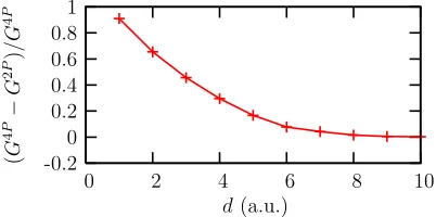
10 8 6 4 2 0 1 0.8 0.6 0.4 0.2 0 -0.2
FIG. 5: (Color-online) The relative difference between the 4-point and 2-point Kohn-Sham conductances. The difference between the two diminishes for opaque barriers.
rection is significant.
Finally we numerically demonstrate the appropriateness of the 2-point conductance, G2P=G[χ]for opaque barriers. The
graph in Fig. 5 clearly shows that for d>4 theF[ ]-dependent
prefactor is very close to 1, which supports our arguments in Sec. V as well as is in agreement with previous numerical work33
VIII. CONCLUSION
In conclusion, we have presented a unified formalism, based on singular character of response functions, that gives the conductance of a general system of interacting electrons. We have derived a closed formula for the 4-point conductance in terms of the many-body response functions: the irreducible conductivity or the irreducible density response. The formula-tion allows for clear demonstraformula-tion of the validity of the
Lan-dauer formula for broadening or opaque nanojunctions. Fur-thermore, we have utilized our formulation for examining the exchange and correlation effects on the conductance within the time-dependent density functional theory. We have shown that the long time limit determines the functional form of the exchange-correlation kernel that can lead to nonzero correc-tions. The exposed theory can be also used for ab-initio cal-culations for which the achievable precision in conductance calculation for a given size of a finite-size simulation cell has been demonstrated on a simple metal-vacuum-metal junction.
Acknowledgments
This research was supported by the Slovak grant agency VEGA (project No. 1/2020/05), the NATO Security Through Science Programme (EAP.RIG.981521) and the EU’s 6th Framework Programme through the NANOQUANTA Net-work of Excellence (NMP4-CT-2004-500198).
IX. APPENDIX: EVALUATION OF FUNCTIONALSF
ANDG.
The functionalsF[ ]andG[ ]were given explicitly in the Fourier-transformed form in Eqs. (9), (10) and Eq. (7) respec-tively. In numerical calculations it is more advantageous and numerically stable to use their representation in real space. To achieve this, we use the inverse transform of the irreducible density response function defined by
χ(q,q′) =
Z dzdz′ 2π e
−iqzχ(z,z′)eiq′z′. (27)
Several times we will have to resolve the integral of the type
f(z0) = Z dq
q e
iqz0χ(q,q′). (28)
Sinceχ(q, .)∼q for small q, the integral is well defined and
we can choose to interpret the apparent singularity 1/q as
1/(q+iδ) or 1/(q−iδ) withδ →0+. Taking the former (the final result is independent of this choice) and using the inverse transform (27) we find
f(z0) =−i Z
dzdz′θ(z0−z)χ(z,z′)eiq ′z′
, (29)
whereθ(z)is the unit step function.
Using the definition ofG[ ]and using the integral (29) twice
with z0=0 we readily obtain
G[χ] = lim
α→0+α
Z 0 −∞
dz
Z ∞ 0
dz′χ(z,z′; iα). (30)
[image:9.612.72.290.49.246.2] [image:9.612.89.290.349.449.2]8
Fourier transform:
F[χ] = α
Z dq
qq′
Z dzdz′ 2π e
−iqzχ(z,z′)eiq′z′
q′=0 (31)
= −iα
Z ∞ 0
dz
Z ∞ −∞
dz′χ(z,z′)e
iq′z′
q′ q′=0
(32)
= α
Z 0 −∞dz
Z ∞ −∞dz
′χ(z,z′)z′ (33)
since we can Taylor expand e−iq′z′ with the linear term giving the only nonzero contribution.
∗ Electronic address: [email protected]
1 J. Taylor, M. M. Brandbyge, and K. Stokbro, Phys. Rev. Lett. 89, 138301 (2002).
2 H. Basch, R. Cohen, and M. A. Ratner, Nano Lett. 5, 1668 (2005). 3 N. Sai, M. Zwolak, G. Vignale, and M. DiVentra, Phys. Rev. Lett.
94, 186810 (2005).
4 J. Jung, P. Bokes, and R. W. Godby, Phys. Rev. Lett. 98, 259701 (2007).
5 C. Toher, A. Filippetti, S. Sanvito, and K. Burke, Phys. Rev. Lett.
95, 146402 (2005).
6 M. Koentopp, K. Burke, and F. Evers, Phys. Rev. B 73, 121403(R) (2006).
7 J. J. Palacios, Phys. Rev. B 72, 125424 (2005).
8 G. Stefanucci and C. O. Almbladh, Phys. Rev. B 69, 195318 (2004).
9 M. DiVentra and T. N. Todorov, J. Phys.: Condens. Matter 16, 8025 (2004).
10 M. Koentopp, C. Chang, K. Burke, and R. Car, cond-mat/0703591v1 (2007).
11 G. Vignale, C. A. Ullrich, and S. Conti, Phys. Rev. Lett. 79, 4878 (1997).
12 P. Delaney and J. C. Greer, Phys. Rev. Lett. 93, 036805 (2004). 13 G. Fagas, P. Delaney, and J. C. Greer, Phys. Rev. B 73, 241314(R)
(2006).
14 A. Ferretti, A. Calzolari, R. DiFelice, F. Manghi, M. J. Caldas, M. B. Nardelli, and E. Molinari, Phys. Rev. Lett. 94, 116802 (2005).
15 P. Darancet, A. Ferretti, D. Mayou, and V. Olevano, Phys. Rev. B
75, 075102 (2007).
16 K. Thygesen and A. Rubio, J. Chem. Phys. 126, 091101 (2007). 17 Y. Meir and N. S. Wingreen, Phys. Rev. Lett. 68, 2512 (1992). 18 R. E. Prange, Phys. Rev. 131, 1083 (1963).
19 F. Malet, M. Pi, M. Barranco, and E. Lipparini, Phys. Rev. B 72, 205326 (2005).
20 E. Prodan and R. Car, cond-mat/0702192 (2007).
21 P. Bokes and R. W. Godby, Phys. Rev. B 69, 245420 (2004). 22 P. Bokes, J. Jung, and R. W. Godby, cond-mat/0604317 (2006). 23 D. J. Thouless, Phys. Rev. Lett. 47, 972 (1981).
24 A. Kamenev and W. Kohn, Phys. Rev. B 63, 155304 (2001). 25 R. Landauer, Z. Phys. B: Condens. Matter 68, 217 (1987). 26 R. Gebauer and R. Car, Phys. Rev. Lett. 93, 160404 (2004).
27 R. Kubo, in Lectures in Theoretical Physics, Vol. 1, edited by W. E.cBrittin and L. G. Dunham (Interscience, New York, 1959). 28 D. Pines and P. Nozieres, The Theory of Quantum Liquids (W. A.
Benjamin, Inc., New York, 1966).
29 G. F. Giuliani and G. Vignale, Quantum Theory of the Electron
Liquid (Cambridge University Press, Cambridge, 2005).
30 G. Mahan, Many-Particle Physics (Kluwer Academic/Plenum Publishers, New York, 2000).
31 R. Landauer, in Analogies in Optics and Micro Electronics, edited by W. van Haeringen and D. Lenstra (Kluwer, Dordrecht, 1990). 32 F. Sols, Phys. Rev. Lett. 67, 2874 (1991).
33 H. Mera, P. Bokes, and R. W. Godby, Phys. Rev. B 72, 085311 (2005).
34 K. Carva and I. Turek, Czech. J. of Physics 54, D257 (2004). 35 P. Nozieres, Theory of interacting Fermi systems (W. A.
Ben-jamin, Inc., New York, 1964).
36 G. Vignale and W. Kohn, Phys. Rev. Lett. 77, 2037 (1996). 37 S. Botti, A. Fourreau, F. Nguyen, Y.-O. Renault, F. Sottile, and L.
Reining, Phys. Rev. B 72, 125203 (2005).
38 L. Reining, V. Olevano, A. Rubio, and G. Onida, Phys. Rev. Lett.
88, 66404 (2002).
39 E. K. U. Gross and W. Kohn, Phys. Rev. Lett. 55, 2850 (1985). 40 J. Jung, P. Garcia-Gonzalez, J. F. Dobson, and R. W. Godby, Phys.
Rev. B 70, 205107 (2004).
41 N. Sai, N. Bushong, R. Hatcher, and M. DiVentra, Phys. Rev. B
75, 115410 (2007).
42 Recently, clear signatures of the resistivity dipoles were found in time-dependent simulations when starting from a charged initial state41.
43 For simplicity of presentation we assume that the induced field inside the electrode is absent, as is exactly true for jellium elec-trodes, used later in Sec. VII. Generalization for an electrode with atomic structure is straightforward: The induced field~Eiis split into the local field induced inside the electrode,~Ei,e(which has an average value zero over the electrode’s unit cell), and the dif-ference~Ei,j=~Ei−~Ei,e. The latter then defines the potential drop according to Eq. 3 and the former needs to be included into the response entering the functionalFσ[σ˜]where ˜σ=σ⋆(1+χe) withχe=δEi,e/δEaux.
44 From here on we use the atomic units with ¯h=m