A framework for power analysis using a structural equation modelling procedure

White Rose Research Online URL for this paper:

http://eprints.whiterose.ac.uk/26/

Article:

Miles, Jeremy (2003) A framework for power analysis using a structural equation modelling

procedure. BMC Medical Research Methodology. ISSN 1471-2288

https://doi.org/10.1186/1471-2288-3-27

[email protected] https://eprints.whiterose.ac.uk/ Reuse

Items deposited in White Rose Research Online are protected by copyright, with all rights reserved unless indicated otherwise. They may be downloaded and/or printed for private study, or other acts as permitted by national copyright laws. The publisher or other rights holders may allow further reproduction and re-use of the full text version. This is indicated by the licence information on the White Rose Research Online record for the item.

Takedown

If you consider content in White Rose Research Online to be in breach of UK law, please notify us by

Methodology

Open Access

Research article

A framework for power analysis using a structural equation

modelling procedure

Jeremy Miles*

Address: Department of Health Sciences, University of York, Heslington, York, YO10 5DD, United Kingdom

Email: Jeremy Miles* - [email protected] * Corresponding author

power analysisstructural equation

Abstract

Background: This paper demonstrates how structural equation modelling (SEM) can be used as a tool to aid in carrying out power analyses. For many complex multivariate designs that are increasingly being employed, power analyses can be difficult to carry out, because the software available lacks sufficient flexibility.

Satorra and Saris developed a method for estimating the power of the likelihood ratio test for structural equation models. Whilst the Satorra and Saris approach is familiar to researchers who use the structural equation modelling approach, it is less well known amongst other researchers. The SEM approach can be equivalent to other multivariate statistical tests, and therefore the Satorra and Saris approach to power analysis can be used.

Methods: The covariance matrix, along with a vector of means, relating to the alternative hypothesis is generated. This represents the hypothesised population effects. A model (representing the null hypothesis) is then tested in a structural equation model, using the population parameters as input. An analysis based on the chi-square of this model can provide estimates of the sample size required for different levels of power to reject the null hypothesis.

Conclusions: The SEM based power analysis approach may prove useful for researchers designing research in the health and medical spheres.

Background

Structural equation modelling (SEM) was developed from work in econometrics (simultaneous equation models; see for example Wansbeek and Meijer [2]) and latent var-iable models from factor analysis [3,4]. Structural equa-tion modelling is an enormously flexible technique – it is possible to use a structural equation modelling approach to carry out direct equivalents of many analyses, including (but not limited to): ANOVA, correlation, ANCOVA, mul-tiple regression, multivariate analysis of variance, and

multivariate regression. This flexibility will be exploited in the approach set out in this article.

A necessarily very brief introduction to the logic of struc-tural equation modelling is presented here – for a more thorough introduction to the basics of structural equation modelling the reader is directed towards one of the many good introductory texts, (Steiger has recently reviewed several such texts [5]). For more details on the statistical and mathematical aspects of structural equation

Published: 11 December 2003

BMC Medical Research Methodology 2003, 3:27

Received: 28 May 2003 Accepted: 11 December 2003

This article is available from: http://www.biomedcentral.com/1471-2288/3/27

modelling, the reader is directed toward texts by Bollen [4] (a second edition of this text is in press) or Wansbeek and Meijer [3] and Jöreskog [7].

The data to be analysed in a structural equation model comprise the observed covariance matrix S, and may include the vector of means M. If k represents the number of variables in the dataset to be analysed, the number of non-redundant elements (p) is given by:

p = k (k + 1)/2 + k

This formula gives the number of non-redundant ele-ments in the covariance matrix (S) and vector of means (M).

However many models exclude the mean vector, and so the number of non-redundant elements in the covariance matrix is given by:

p = k (k + 1)/2

The model is a set of r parameters, fixed to certain values (usually 0 or 1), constrained to be equal to one another, or allowed to be free. The estimated parameters of the model are used to calculate an implied covariance matrix,

Σ and an implied vector of means. An iterative search is carried out, which attempts to minimise the discrepancy function (F), a measure of the difference between S and Σ. The discrepancy function (maximum likelihood, for cov-ariances only) is given by:

F = log |Σ| + tr (SΣ-1_{) - log |S| - p}

The discrepancy function, multiplied by N - 1, follows a χ2

distribution, with degrees of freedom (df) equal to p - r. The value of the discrepancy function multiplied by N - 1 is usually referred to as the χ2 _{test of the model.}

In addition to the χ2 _{test, standard errors (and hence}

t-val-ues [although these valt-val-ues are referred to as t-scores, they are more properly described as asymptotic z-scores] and probability values) can be calculated, and these can be used to test the statistical significance of the difference between that parameter value, and any hypothesised pop-ulation value (most commonly zero).

When p >r, the model is referred to as being over-identi-fied, in this case it will not necessarily be possible (or usual) to find values for the set of parameters, r, which can ensure that S = Σ. However, where r = p it is possible (given that the correct parameters are estimated) to provide val-ues for the parameters in the model, such that S = Σ. This type of model, where r = p is described as being just

iden-tified. The df of the model will be equal to zero, and the value of χ2 _{will also be equal to zero.}

It is possible to use the standard errors of the parameter estimates to test the statistical significance of the values of these parameters. In the next section, we shall see how it is also possible to use the χ2 _{test to evaluate hypotheses}

regarding the value of these parameters in a model. This is most easily described using path diagrams as a tool to rep-resent the parameters in a structural equation model.

The commonest representation of a structural equation model is in a path diagram. In a path diagram, a box rep-resents a variable, a straight, single-headed arrow repre-sents a regression path, and a curved arrow reprerepre-sents a correlation or covariance (in addition, an ellipse repre-sents a latent, or unobserved variable; the methods described in this paper do not use latent variables, how-ever the interested reader is directed towards a recent chapter by Bollen [3]). Different conventions exist for path diagrams – throughout this paper the RAM specifica-tion will be used (Neale, Boker, Xie and Maes, give a full description of this approach. [8]) In RAM specification, a double headed, curved arrow, which curves back to the same point represents the variance of the variable (the covariance of a variable with itself being equal to the var-iance). In the case of an endogenous (dependent) varia-ble, the variance represents the residual, or unexplained variance of the variable.

Methods

In order to estimate a correlation, a covariance is esti-mated, which can then be standardised to give the corre-lation. If all variables are standardised, the covariance is equal to the correlation. The model that is estimated when a covariance is calculated can be represented in path dia-gram format as two variables, linked with a curved, dou-ble headed arrow, as shown in Figure 1. Each of the variables also has a double-headed arrow which repre-sents the variance of the variable. There are three esti-mated parameters – the magnitude of the covariance, and the variance of each of the two variables x and y. The model input is also three statistics – the covariance, and the variance of the two variables. Therefore p – the number of statistics in the data, and r, the number of parameters in the model are both equal to 3. There are therefore 0 df, and the model is just identified. The esti-mate of the magnitude of the covariance, along with its confidence intervals, can then be used to make inferences about the population, and test for statistical significance.

estimate of y on x, and the unexplained variance of y

(equivalent to 1 - R2_{). Again, the estimate of the}

parame-ter, along with the confidence intervals, can be used to make inferences to the population and test for statistical significance.

A multiple regression model is shown in Figure 3. Here there are 4 predictor variables (x1 to x4) which are used to

predict an outcome variable (y). There are 5 variables in the model, and therefore the data comprise 15 elements (5 variances and 10 covariances), and p = 15. The model comprises 4 variances of the predictor variables, 1 unex-plained variance in the outcome variable, 4 regression weights, and 6 correlations amongst the independent var-iables. Therefore, r = p = 15, and the model is just identi-fied. Two different kinds of parameters are usually tested for statistical significance in this model. First, the unex-plained variance in the outcome variable is tested against 1 (if standardised) to determine whether the predictions that can be made from the predictor variables is likely to be better than chance. This is the equivalent of the ANOVA test of R2 _{in multiple regression. Second, the}

values of the individual regression estimates can be tested for statistical significance.

Any analysis of variance model can also be modelled as a regression model [9,10], hence all multiple regression / ANOVA models can be incorporated into the general framework.

The logic extends to the case of a multivariate ANOVA or regression, which has multiple outcome variables. The multivariate approach allows each of the individual paths to be estimated, and tested for statistical significance, however, it also allows groups of paths to be tested simul-taneously, using the χ2 _{difference test – the multivariate F}

test in MANOVA is equivalent to the simultaneous test of all of the paths from the predictor variables to the outcome variables. The multivariate test can prove more powerful than two separate univariate analyses [11].

When a model is restricted – that is not all paths are free to be estimated, it becomes over-identified. The difference between the data implied by the model and the observed data can be tested for statistical significance using the χ2

test. Each restriction in the model adds 1 df, and this can be used to interpret the difference between the data implied by the model, and the observed data.

The simplest example of this is in the case of the correla-tion (Figure 1). Using data from a recent study (Wolfradt, Hempel and Miles [12]), I calculate the correlation between active coping and passive coping. I find that r = -0.049, with N = 271, and p = 0.422. Carrying out the same analysis (using standardised variables) in a SEM package (AMOS 4.0 [13]) I find that the estimated correlation is -0.049, with a standard error of 0.06, and an associated probability value of 0.422. The answers being exactly equivalent. However, the structural equation modelling approach enables me to consider the problem in a differ-ent way. In the model, I can restrict the correlation between the two measures to zero. Because the model now has a restriction added to it, r <p and the model is over-identified. The discrepancy can be assessed, using the discrepancy function F, and tested using a χ2 _{test, with 1}

df (the number of restrictions in the model). When this is done, the χ2 _{associated with the test is equal to 0.65,}

which, with 1 df, has an associated probability of 0.421. The three approaches lead to equivalent conclusions and identical (within rounding error) probability values. However, the third approach – that of using the χ2 _test,

gives an additional advantage – that it is possible to fix more than one parameter to a pre-specified value (usually, but not always, 0).

In a multivariate regression, a set of outcomes is regressed on a set of predictors. As well as including a test of each parameter, a multivariate test is also carried out, testing the effect of each predictor on each set of outcome varia-bles. Again using data from Wolfradt, et al., I carried out a multivariate regression (using the SPSS GLM procedure). The three predictor variables were mother's warmth,

Covariance between x and y

Figure 1

Covariance between x and y.

A regression analysis, with one independant variable

Figure 2

mother's rules, and mother's demands. The two outcomes were active coping and passive coping.

Four models were estimated, in the first, all parameters were free to be estimated. In the second, the two paths from warmth were restricted to zero, in the second, the two paths from rules were restricted to zero, and in the final model, the two paths from demands were restricted to zero. The first model has 0 df, and hence the implied and observed covariance matrices are always equal, and the χ2 _{is equal to zero. Each of the other models has 2 df,}

because two restrictions were added to the model.

The results of the tests are shown in Table 1. This shows the results from the multivariate GLM (carried out in SPSS) and the SEM approaches. The GLM results provide a multivariate F and an associated p value, shown in the first pair of columns in Table 1. The SEM results provide a

χ2 _{and associated p-value, shown in the second pair of}

col-umns in Table 1. The two sets of tests are, as can be seen, very close to one another, in terms of the levels of statisti-cal significance.

In addition to relationships between variables being incorporated into structural equation models it is also possible to incorporate means (or, in the case of endog-enous variables, intercepts). In the RAM specification, a mean is modelled as a triangle. The path diagram shown in Figure 4 effectively says "estimate the mean of the vari-able x". In the circumstances where there are no restrictions, the estimated mean of x in the model will be the mean of x in the data. However, it is possible to place restrictions on the data, and test the model, again with a

χ2 _{test. A simple example would be to place a restriction}

on the mean to a particular value – this would be the equivalent of a one sample t-test. A further example, shown in Figure 5 is a paired samples t-test. Here, the means are represented by the parameter a – both paths are given the same label, meaning that the two means are fixed to be equal. Again, this can be estimated with a χ2

test.

A one way repeated measures ANOVA is also possible, using the same logic. The path diagram is shown in Figure 6. Here, the null hypotheses (that µ1 = µ2 = µ3) is tested by

fixing the parameters a, b and c to be equal to one another. It is also possible to carry out post-hoc tests, to compare each of the individual means.

This model was tested using the first 20 cases from Wolf-radt, et al [12]. (This number of cases was chosen for illus-trative purposes – to demonstrate that the equivalence of results is not dependent upon having large samples.) The three variables compared were mother's rules, mother's demands, and mother's warmth. The means and covariances are shown in Table 2. Again, the analysis was carried out using the GLM (repeated measures) procedure in SPSS and within a SEM package (Mx). The results for the four null hypotheses tested using the SPSS GLM pro-cedure, and using the model with restrictions described above in Mx [8], are shown in Table 3. The first null hypothesis tested is that the means of all three variables

Table 1: Results of multivariate F test, and χ2 _{difference test, for multivariate regression}

GLM Results SEM results

Multivariate F (df = 2, 263) p χ2 _{(df = 2) p}

Rules 0.23 0.794 0.47 0.791

Demands 5.3 0.005 10.6 0.005

Warmth 10.7 <0.001 20.9 <0.001

Multiple regression representation of path diagram

Figure 3

are equal (in the population). The three further tests examine differences between pairs of variables. Again, the GLM approach gives an F statistic, and associated p-value; the SEM approach gives a χ2 _{statistic, and associated}

p-value. Again, the p-values from both of these approaches are very similar, demonstrating the equivalence of the two approaches.

The SEM analyses considered so far have only considered single groups, however, it is possible to carry out analyses across groups, where the parameters in two (or more) groups can be constrained to be equal. This multiple group approach can be used to analyse data from a mixed design, with a repeated measures factor, and an independ-ent groups factor. The model is shown in Figure 7 (again using the data from Wolfradt, et al.). There are data from two groups, males and females. Each group has measures

taken on two variables (x1 and x2). The parameter labelled

b in the males represents the intercept of the two variables

x₁ and x₂, which in this case is the mean of x₂, the param-eter labelled a is the slope parameter, or the difference between the means of x1 and x2. There are three separate

hypotheses to test:

1) Main effect of sex.

2) Main effect of type (x₁ vs x₂)

3) Interaction effect of type and sex.

Again, using SPSS a mixed ANOVA can be carried out – the results of which are shown in Table 5. To carry out the equivalent analysis in an SEM context is slightly more complex. A series of models need to be estimated, with increasing numbers of restrictions. These models are nested, and the differences between the models provides a test of the hypotheses.

Model 1: b = d, a = c = 0. This model has three restrictions, and hence 3 df.

Model 2: a = c = 0. This model has two df. By removing the

b = d restriction, the means of the two measures are allowed to vary across the groups.

Estimating the mean

Figure 4

Estimating the mean.

Representation of paired samplest test in path diagram format

Figure 5

Representation of paired samplest test in path dia-gram format.

Path diagram representation of one way repeated measures ANOVA with three independant variables

Figure 6

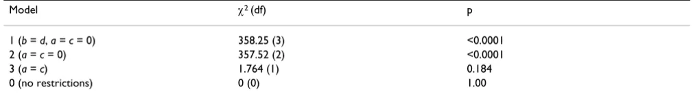
Model 3: a = c. This model has one df. By removing the a

= c = 0 restriction, the means of rules and demands are allowed to vary. However, because the a = c restriction is still in place, the variation is forced to be equal across groups. The χ2 _{difference test between this model and}

model 2 provides the probability associated with the null hypothesis that there is no effect of rules vs demands (type).

Model 0: All parameters free. This model has zero df, and hence χ2 _{will equal zero. The} χ2 _{difference test between}

this model and model 3 tests the interaction effect, although this will be equal to the χ2 _{and df of model 3.}

This allows the difference between x₁ and x₂ to vary across gender, thereby testing the null hypothesis of no interac-tion effect.

These 4 models were estimated using the data from Wolf-radt, et al. The type distinction was mother's rules versus

mother's warmth. The results of each of these model tests are shown in Table 4 and the differences between the models, which give the tests for the main effects and inter-actions, are shown in Table 5. Again, the GLM test and the SEM test are giving very similar (although not identical) results. The effect of sex, is found to be non-significant by both tests (p = 0.31 for the F test, and 0.39 for the SEM test. The result for the type difference is found to be highly significant by both the F test (p < 0.001) and the SEM test (p < 0.001), and finally the sex x type interaction is statis-tically nonsignificant for the F test (p = 0.186) and the SEM test (p = 0.184).

Power Analysis

The power of a statistical test is the probability that the test will find a statistically significant effect in a sample of size N, at a pre-specified level of alpha, given that an effect of a particular size exists in the population. Power of statisti-cal tests is considered increasingly important in medistatisti-cal

Table 2: Means and covariances of warmth, demands and rules (variances are shown in the diagonal)

Warmth (1) 0.37168421

Demands (2) 0.17187970 0.24575725

Rules (3) -0.21171930 -0.05423559 0.24814035

µ 1.9700 2.6571 2.9733

Warmth (1) Demands (2) Rules (3)

Table 3: Comparison of results from GLM test carried out using SPSS and test using SEM framework, using Mx.

GLM Test Mx Test

Null Hypothesis F (df) p χ2 _{(df) p}

1. µ1 = µ2 = µ3 (rules = demands = warmth) 16.530 (2, 18) 0.000084 19.8 (2) 0.000050

2. µ1 = µ2 (rules = demands) 34.5 (1, 19) 0.00012 19.7 (1) 0.000009

3. µ1 = µ3 (rules = warmth) 19.29 (1, 19) 0.00031 13.31 (1) 0.00026

4. µ2 = µ3 (demands = warmth) 3.32 (1, 19) 0.084 3.06 (1) 0.080

Notes: 1_{Result from multivariate test} 2_{Large number of decimal places have been given to illustrate similarity of probability values based on two}

methods.

Table 4: χ2_{, df and p for models 0 to 4. Differences between these models are used to test hypotheses of main effects and interactions)}

Model χ2 _{(df) p}

1 (b = d, a = c = 0) 358.25 (3) <0.0001

2 (a = c = 0) 357.52 (2) <0.0001

3 (a = c) 1.764 (1) 0.184

and social sciences, and most funding bodies insist that power analysis is used to determine the appropriate number of participants to use. It is increasingly recognised that power is not just a statistical or methodological issue, but an ethical issue. In medical trials, patients give their consent to take part in studies which they hope will help others in the future – if the study is underpowered, the probability of finding an effect may be minimal. The CONSORT statement (CONsolidated Standards Of Reporting Trials [16]), a checklist adopted by a large number of medical journals (see http://www.consort-statement.org), states that published research should give a description of the method used to determine the sample size. Whilst the basis for power calculations is relatively simple, the mathematics behind them is complex, as they require calculation of areas under the curve for non-cen-tral distributions.

[When using statistics for any amount of time, we become familiar with central distributions – these are distribu-tions such as the t, the F or the χ2_{. However, these are the}

distribution of the statistic when the null hypothesis is true. To calculate the distribution when the null hypothesis is false, we must know the non-centrality parameter – the expected mean value of the distribution, and then examine the probability of finding a result which would be considered significant at our pre-specified level of alpha.]

Whilst it is possible in some statistical packages to calcu-late values for non-central distributions, it is not straight-forward (although it is possible) to use these for power calculations.

There are a range of resources available for power analysis, including commercial books containing tables [16-19], commercial software (e.g. SamplePower, nQuery), free-ware softfree-ware (e.g. GPower [14]), and web pages which implement the routines. However, software for power analysis has some problems coping with the range of complex designs that are possible in research. Including covariates in a study can increase the power to detect a difference [20] but can also increase the complexity of the power analysis. In a multiple regression analysis, calcula-tion of the power to detect a statistically significant value for R2 _{is relatively straightforward, using tables or books.}

However, the power to detect significant regression weights for the individual predictors is more difficult. Incorporating interactions into power analysis is also not straightforward.

A multivariate design can also have more power than a univariate design, but the power of the design is affected in complex ways by the correlation between the outcome variables [6]. Most software packages do not have suffi-cient flexibility to incorporate these effects.

Power from SEM

An alternative way to approach power is to use a structural equation modelling framework. Satorra and Saris [1] pro-posed a procedure for estimating power for structural equation models, which is as follows:

First, a model is set up which matches the expected effect sizes in the study. From this the expected means and covariances are calculated. These data are treated as popu-lation data. Second, a model is set up where the parame-ters of interest are restricted to zero (or the values expected under the null hypothesis). This model is then estimated, and the χ2 _{value of the discrepancy function is calculated.}

This can be used to calculate the non-centrality parameter, which is then used to estimate the probability of detecting a significant effect. It should be noted that the power estimates using the SEM approach are asymptotically equivalent to the GLM approach employed in OLS

mod-Table 5: Results of multivariate F test, and χ2 _{difference test, for multivariate regression}

Multivariate F (df = 1, 266) p χ2 _{given by:} χ2 _{(df = 1) p}

Sex 1.4 0.310 Model 2 - Model 1 0.73 0.393

Type (rules vs demands) 739.1 <0.001 Model 3 - Model 2 355.8 <0.001

Sex x Type 1.76 0.186 Model 3 - Model 0 1.76 0.184

Structural equation model for a mixed ANOVA

Figure 7

elling, at smaller sample sizes, larger discrepancies will occur between the two methods [21].

Much of this is automated within the structural equation modelling program Mx [8], which is available for free, and can be downloaded from http://www.vcu.edu/mx/.

Three examples of power analysis are presented. Example 1 shows how to use SEM to power a study to detect a cor-relation; the second is used for a mixed ANOVA, using a 2 × 2 design; the third shows how to power a study that uses a multivariate ANOVA / regression.

Example 1

In example 1, I estimate the probability of detecting a population correlation of size r = 0.3 ([see additional file 1]). For a simple model, such as this, it is not necessary to calculate the expected population correlation matrix – the correlation is simply 0.3. The sample size required for different levels of power is shown in Table 6, along with estimates calculated by GPower and and nQuery Advisor 4.0. The figures provided for the sample size from each method are very similar, although not identical.

Example 2: Multivariate ANOVA

The second example to be examined is the case of a mul-tivariate ANOVA. It is well known that a mulmul-tivariate design can be more powerful than a univariate design, though calculating how much more powerful can be dif-ficult. [21]

The simple multivariate design is shown in Figure 8. Here the effects of a single independent variable on three dependent variables are assessed. It is necessary to calculate the population covariance matrix for this exam-ple. The covariance matrix of the dependent variables is found by multiplying the vector of regression weights by its transpose, and adding the residual variances and covar-iances of the dependent variables.

The correlations between the dependent variables is there-fore given by:

It is usually more straightforward to enter the values as fixed parameters into the SEM program, and estimate the population covariance matrix in this way.

This analysis can proceed via one of two means – three univariate analyses or one multivariate analysis. Calculation of power for the univariate analysis by con-ventional methods (power analysis table or program) is uncomplicated, however calculation of power for the multivariate approach is less so.

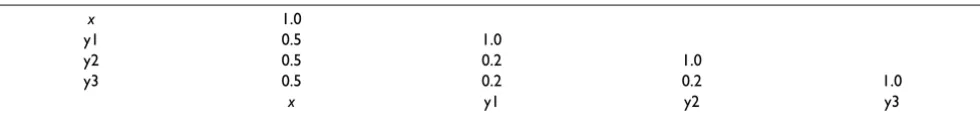
Power can be estimated for two different types of effects. First, the power to detect each of the univariate effects can be examined, second the power to detect the multivariate effect of x on the three dependent variables simultaneously. For the purposes of this example, the standardised population parameter estimates were as fol-lows: each of the standardised univariate effects was equal to 0.5, and the three residual correlations between the dependent variables were set to -0.05.

If all variances are standardised, the implied population covariance matrix is shown in Table 7.

Power estimates can be derived for four separate tests. Three (univariate) tests of each parameter, and one multi-variate test of the three parameters simultaneously. The Mx scripts are available for download in the additional files section example 2 – univariate.mx [see additional file 2] and example 2 – multivariate.mx [see additional file 3]. Power was calculated in two ways: the first approach was to use Mx, as described, the second, for the univariate data only, was to use Nquery, and the results of these analyses are presented in Table 8. (Note that as the population parameters are equal for each of the outcome variables, the analysis for each of the outcomes will be the same, and only one is presented).

Table 6: Power to detect a population correlation r = 0.3, by three programs

Power Mx (SEM approach) GPower nQuery

.25 18 19 21

.50 41 41 44

.75 74 73 76

.80 84 82 85

.90 113 109 113

.95 139 134 139

.99 197 188 195

. . . . . . . . . . . . . . . 5 5 5

5 5 5

75 05 05 05 75 05 05 05 75

         

(

)

1 00 20 20 20 1 00 20 20 20 1 00

. . .

. . .

An extension of this analysis is to be able to relatively sim-ply examine the effects on power of varying the correla-tion between the measures in a multivariate ANOVA. To carry out this analysis, the values of the population correlations between the outcome variables are altered, and the effects on the power noted. Table 9 shows the sample size required for 80% power, given the same regression parameters as in the previous example, but varying correlations between the outcomes. The power required is maximised when the correlations between the outcomes is 0, and as the correlation increases, the power decreases.

Example 3: Repeated Measures ANOVA: The effect of the correlation between variables

Repeated measures analysis presents a number of addi-tional challenges to the researcher, in terms of both meth-odological issues [22] and statistical issues [11]. In a repeated measures analysis, the researcher must examine both the difference between the means of the variables,

and also the covariance/correlation between the variables. In Example 3, I examine the effect of differences in the magnitude of the correlation between variables in a repeated measures ANOVA, comparing the mean of three variables.

The three variables x₁, x₂ and x₃, have population means of 0.8, 1.0 and 1.2 respectively, and variances of 1.0. The correlations between them were fixed to be equal in all

Table 7: Standardised population covariance matrix for example 2

x 1.0

y1 0.5 1.0

y2 0.5 0.2 1.0

y3 0.5 0.2 0.2 1.0

x y1 y2 y3

Table 8: Power for univariate and multivariate tests

Sample size required for 80% power

Mx NQuery

Test that x → y1 = 0 (univariate) (df = 1) 28 26

Multivariate test (df = 3) 14 Note 1

Notes: 1 Power for a multivariate test cannot be calculated using standard software.

Table 9: Relationship between correlation between DVs and Sample size required for 80% power, in multivariate ANOVA.

Correlation between DVs Sample size required for 80%

Power

0.0 8

0.2 14

0.4 21

0.6 27

0.8 33

Multiwariate experimental design, with one independant vari-able (x) and three dependant varivari-ables (y1, y1, y2)

Figure 8

models, and were fixed to be 0, 0.2, 0.8, or -0.2. A simple analysis was carried out, to investigate the sample size required to attain 80% power to detect a statistically sig-nificant difference, at p < 0.05, using an Mx script example 3 [see additional file 4]. The correlation between the vari-ables was estimated to be 0.0, 0.2, 0.5, 0.8 or -0.2.

The results of the analysis are shown in Table 10. This demonstrates that as the correlation increases, the power of the study to detect a difference increases, and the sam-ple size required decreases dramatically.

Concluding Remarks

This paper has presented an approach to power analysis developed by Saris and Satorra for structural equation models, that can be adapted to a very wide range of designs. The approach has three related applications.

First, in carrying out power analyses for studies, there are frequently complex relationships between different relationships in different studies. For example, the power to detect a difference in a repeated measures design is dependent upon the correlation between the variables. It may be possible to give power estimates based on 'best guess' and on upper and lower limits for these measures.

Second, for some types of studies, adequate power analy-sis is very complex using other approaches. To investigate, for example, the power to detect a significant difference between two partial correlations is difficult to calculate.

Third, and finally, in planning instruments to use in research. Many applied areas of research in health have multiple potential outcome measures; for example consider the range of instruments available for the assess-ment of quality of life. Many of these measures will have been used together in previous studies, and therefore the correlation between them may be known, or able to be estimated. The effect of these correlations on the power of the study can be investigated using this approach, which may affect the choice of measure.

For those unfamiliar with the package, and perhaps unfa-miliar with SEM, the learning curve for Mx can be steep. The path diagram tool within Mx is extremely useful – the model is drawn, and restrictions can be added. The pro-gram will then use the diapro-gram to produce the Mx syntax which can then be edited. This approach leads to faster, and more error-free, syntax. The author is happy to be contacted by email to attempt to assist with particular problems that readers may encounter. A document is available which describes how SPSS can be used to calculate the power, given the χ2 _{of the model [see}

addi-tional file 5].

Finally, for readers who may be interested in further exploration of these issues, it should be noted that an alternative approach to estimating fit in SEM has been presented by MacCallum, Browne and Sugawara. [26]

Competing Interests

None declared.

Additional material

Table 10: Variation in power for repeated measures design given different level of correlation between measurements.

Size of correlations between variables Sample size required for 80% power

0.0 125

0.2 101

0.5 65

0.8 29

-0.2 149

Additional File 1

Example 1.mx: Contains Mx syntax to run example 1.

Click here for file

[http://www.biomedcentral.com/content/supplementary/1471-2288-3-27-S1.mx]

Additional File 2

Example 2 – univariate.mx: Contains Mx syntax to run example 2, univariate.

Click here for file

[http://www.biomedcentral.com/content/supplementary/1471-2288-3-27-S2.mx]

Additional File 3

Example 2 – multivariate.mx: Contains Mx syntax to run example 2, multivariate.

Click here for file

[http://www.biomedcentral.com/content/supplementary/1471-2288-3-27-S3.mx]

Additional File 4

Publish with BioMed Central and every scientist can read your work free of charge

"BioMed Central will be the most significant development for disseminating the results of biomedical researc h in our lifetime."

Sir Paul Nurse, Cancer Research UK

Your research papers will be:

available free of charge to the entire biomedical community

peer reviewed and published immediately upon acceptance

cited in PubMed and archived on PubMed Central

yours — you keep the copyright

Submit your manuscript here:

http://www.biomedcentral.com/info/publishing_adv.asp

BioMed_central

Acknowledgements

Thanks to Diane Miles and Thom Baguley, for their comments on earlier drafts of this paper, and to Keith Widaman and Frühling Rijsdijk who reviewed this paper, pointing out a number of areas where clarifications and improvements could be made.

References

1. Satorra A, Saris WE: The power of the likelihood ratio test in covariance structure analysis.Psychometrika 1985, 50:83-90. 2. Wansbeek T, Meijer E: Measurement error and latent variables

in econometrics: Advanced textbooks in economics, 37. Amsterdam: Elsevier 2000.

3. Bollen KA: Latent variables in psychology and the social sciences.Annual Review of Psychology 2002, 53:605-634.

4. Bollen KA: Structural equations with latent variables. New York: Wiley Interscience 1989.

5. Steiger J: Driving fast in reverse: The relationship between software development, theory, and education in structural equation modelling.Journal of the American Statistical Association

2000, 96:331-338.

6. Cole DA, Maxwell SE, Arvey R, Salas E: How the power of MANOVA can both increase and decrease as a function of the intercorrelations among the dependent variables. Psycho-logical Bulletin 1994, 115:465-474.

7. Jöreskog KG: A general approach to confirmatory maximum likelihood factor analysis.Psychometrika 1969, 34:183-202. 8. Neale MC, Boker SM, Xie G, Maes HH: Mx: Statistical Modelling

[computer program].Virginia Institute for Psychiatric and Behavior Genetics, Virginia University 1999.

9. Miles JNV, Shevlin M: Applying regression and correlation analysis.London: Sage 2001.

10. Rutherford A: Introducing ANOVA and ANCOVA: a GLM approach.London: Sage 2001.

11. Stevens J: Applied multivariate statistics for social scientists. Hillsdale, NJ: Erlbaum 1996.

12. Wolfradt U, Hempel S, Miles JNV: Perceived parenting styles, depersonalization, anxiety and coping behaviour in normal adolescents.Personality and Individual Differences 2003, 34:521-532. 13. Arbuckle J: AMOS 4.0 [computer program].Chicago: Smallwaters

1999.

14. Faul F, Erdfelder E: GPOWER: A priori, post-hoc, and compro-mise power analyses for MS-DOS [Computer program]. Bonn, FRG: Bonn University, Dep. of Psychology 1992.

15. Cohen J: Statistical power analysis for the behavioural sciences.Hillsdale, NJ: Erlbaum 21988.

16. Moher D, Schulz KF, Altman DG et al.: The CONSORT state-ment: revised recommendations for improving the quality of reports of parallel group randomised controlled trials.The Lancet 2001, 357:1191-1194.

17. Kraemer HC, Thiemann S: How many subjects? Statistical power analysis in research.Newbury Park, CA: Sage 1987. 18. Machin D, Campbell MJ, Fayers PM, Pinol APY: Sample size tables

for clinical studies.Oxford: Blackwell 21997.

19. Murphy KR, Myors B: Statistical power analysis: a simple and general model for traditional and modern hypothesis tests. Hillsdale, NJ: Erlbaum 1998.

20. Taylor MJ, Innocenti MS: Why covariance: A rationale for using analysis of covariance procedures in randomised studies. Jour-nal of Early Intervention 1993, 17:455-466.

21. Kaplan D, Wenger RN: Asymptotic independence and separa-bility in covariance structure models: implications for speci-fication error, power and model modispeci-fication. Multivariate Behavioral Research 1993, 28:467-482.

22. Keren G: Between- or within-subjects design: a methodologi-cal dilemma. In: A handbook for data analysis in the behavioural sci-ences: methodological issues Edited by: Keren G, Lewis C. Hillsdale, NJ: Erlbaum; 1994.

23. Muthén B, Muthén L: Mplus, 2.0 [computer program].Los Ange-les, CA: Muthén and Muthén 2001.

24. Kaplan D: Statistical power in structural equation modeling.

In: Structural Equation Modeling: Concepts, Issues, and Applications Edited by: Hoyle RH. Newbury Park, CA: Sage Publications, Inc; 1995. 25. Bollen KA: Latent variables in psychology and the social

sciences.Annual Review of Psychology 2002, 53:605-634.

26. MacCallum RC, Browne MW, Sugawara HM: Power analysis and determination of sample size for covariance structure modelling.Psychological methods 1996, 1:130-149.

Pre-publication history

The pre-publication history for this paper can be accessed here:

http://www.biomedcentral.com/1471-2288/3/27/prepub Click here for file

[http://www.biomedcentral.com/content/supplementary/1471-2288-3-27-S4.mx]

Additional File 5

Appendix: Description of adaptation of approach for other programs.

Click here for file