White Rose Research Online URL for this paper: http://eprints.whiterose.ac.uk/2082/
Monograph:
May, A.D., Marler, N., Shepherd, S. et al. (1 more author) (1999) Project FATIMA Final Report: Part 2. Working Paper. Institute of Transport Studies, University of Leeds , Leeds, UK.
Working Paper 531B
[email protected] https://eprints.whiterose.ac.uk/
Reuse
Unless indicated otherwise, fulltext items are protected by copyright with all rights reserved. The copyright exception in section 29 of the Copyright, Designs and Patents Act 1988 allows the making of a single copy solely for the purpose of non-commercial research or private study within the limits of fair dealing. The publisher or other rights-holder may allow further reproduction and re-use of this version - refer to the White Rose Research Online record for this item. Where records identify the publisher as the copyright holder, users can verify any specific terms of use on the publisher’s website.
Takedown
If you consider content in White Rose Research Online to be in breach of UK law, please notify us by
White Rose Research Online
http://eprints.whiterose.ac.uk/Institute of Transport Studies University of Leeds
This is an ITS Working Paper produced and published by the University of Leeds. ITS Working Papers are intended to provide information and encourage discussion on a topic in advance of formal publication. They represent only the views of the authors, and do not necessarily reflect the views or approval of the sponsors.
White Rose Repository URL for this paper: http://eprints.whiterose.ac.uk/2082/
Published paper
A D May, N Marler, S Shepherd & P Timms(1999) Project FATIMA Final Report: Part 2. Institute of Transport Studies, University of Leeds, Working Paper 531B
Deliverable D4:
Final Report Part 2
Status : P
PROJECT
FATIMA
Contract No. UR 97 SC 1015
Project
Institute for Transport Studies
Co-ordinator:
University of Leeds
Partners:
TUW/IVV
VTT
CSST
TT-ATM
TØI
Date:
12th February 1999
file: fatima/fin12pt2.doc
PROJECT FUNDED BY THE EUROPEAN COMMISSION UNDER THE TRANSPORT RTD PROGRAMME OF THE
CONTENTS
1. INTRODUCTION AND BACKGROUND 6
1.1 Introduction to Part 2 6
1.2 Options for private finance in transport 6
1.2.1 General 6
1.2.2 What is private finance and why use it? 7
1.2.3 Risks 7
1.2.4 Division of responsibility 8
2. DEFINITION OF OBJECTIVE FUNCTIONS 10
2.1 Overview of objective functions 10
2.1.1 The role of the Benchmark Objective Function, and links to OPTIMAError! Bookmark not defined. 2.1.2 The role of the other objective functions in FATIMA Error! Bookmark not defined.
2.2 Present Value of Finance (PVF) 10
2.3 Economic Efficiency Function (EEF) 11
2.4 Economic Efficiency Objective Function with external costs (EEFP) 12
2.5 Sustainability Objective Function (SOF) 14
2.6 Benchmark Objective Function (BOF) Error! Bookmark not defined.
2.7 Constrained Objective Function (COF) Error! Bookmark not defined.
2.8 Regulated Objective Function (ROF) Error! Bookmark not defined.
2.9 Deregulated Objective Function (DOF) 16
2.10 Half regulated Objective Function (HOF) 17
2.11 City specific definitions of HOF 17
2.12 Non-modelled benefits and disbenefits 18
3. POLICY MEASURES 18
3.1 Summary of measures 18
3.2 Measures tested in the optimisation process 19
4. OVERVIEW OF TRANSPORT MODELS USED 22
5. RESULTS FOR THE NINE CITIES 23
5.1 Overview of the Optimisation Method 23
5.1.1 Edinburgh 23
5.1.2 Merseyside 24
5.1.3 Vienna and Eisenstadt 24
5.1.5 Tromsø 25
5.1.6 Helsinki 26
5.1.7 Salerno 26
5.1.8 Torino 27
5.2 Results 27
5.3 Summary table - best BOF Error! Bookmark not defined.
5.4 Summary table - best COF Error! Bookmark not defined.
5.5 Summary table - best ROF Error! Bookmark not defined.
5.6 Summary table - best DOF Error! Bookmark not defined.
5.7 Summary table - best HOF Error! Bookmark not defined.
5.8 Comments on results 34
5.8.1 Regulated regimes 34
5.8.2 Deregulated regimes 35
5.9 Comparison of policies by city and objective function 35
5.9.1 Edinburgh 36
5.9.2 Merseyside 36
5.9.3 Vienna 37
5.9.4 Eisenstadt 37
5.9.5 Tromsø 37
5.9.6 Oslo 38
5.9.7 Helsinki 38
5.9.8 Torino 39
5.9.9 Salerno 39
5.10 Comparison across cities by function 43
BOF* solutions 43
ROF* and COF* solutions 44
5.10.3 HOF* solutions 44
5.10.4 DOF* solutions 45
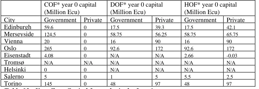
5.11 Financial Implications of Value Capture and PVF 49
5.11.1 General 49
5.11.2 Availability of finance in year zero 49
5.12 Changes in car-km by function 50
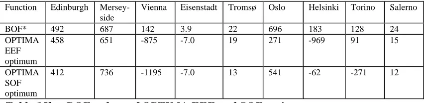
6. OPTIMA : EEF AND SOF OPTIMA 51
6.1 Changes between OPTIMA and FATIMA 51
6.2 Edinburgh 53
6.3 Merseyside 53
6.4 Vienna 54
6.5 Eisenstadt 54
6.6 Tromsø 55
6.8 Helsinki 55
6.10 Salerno 57
6.11 Summary and conclusions 58
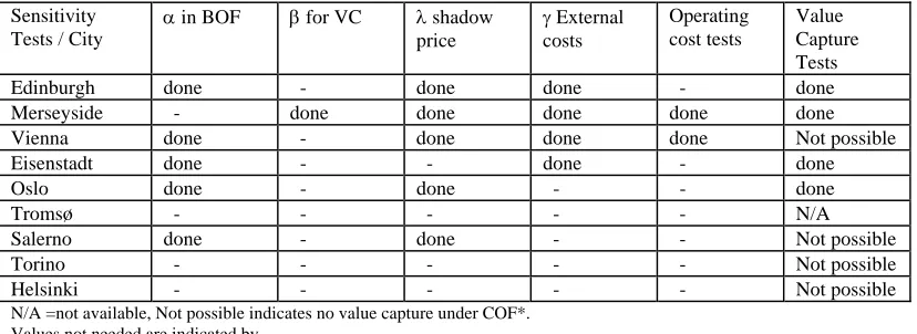
7. SENSITIVITY TESTS 59
7.1 The shadow price λ 59
7.2 α in BOF 60
7.3 β for Value Capture 60
7.4 The external costs basis γ 61
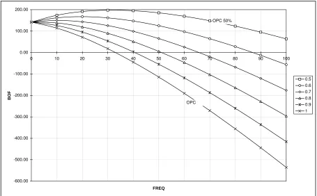
7.5 Operating costs 62
7.6 An alternative approach to Value Capture (AVC) 65
8. FEASIBILTY AND ACCEPTABILITY 67
8.1 The consultation process 67
8.2 Feasibility and acceptability for individual cities 68
8.2.1 Edinburgh 68
8.2.2 Merseyside 70
8.2.3 Vienna 72
8.2.4 Eisenstadt 73
8.2.5 Helsinki 74
8.2.6 Torino 76
8.2.7 Salerno 77
8.3 Overall feasibility 79
8.3.1 Financial feasibility 79
8.3.2 Technical feasibility 79
8.3.3 Legislative feasibility 79
8.4 Overall acceptability 79
8.4.1 Public acceptability 80
8.4.2 Political acceptability 80
8.4.3 Private sector acceptability 80
8.4.4 Operator acceptability 81
8.4.5 Quality issues 81
8.5 Comments on the methodology 81
8.6 Applicability to other member states 82
8.6.1 General 82
8.6.2 Stockholm 82
8.6.3 Berlin 84
8.6.4 Implications of the Stockholm and Berlin consulatations 86
9. LITERATURE 87
9.1 References 93
9.2 Bibliography 93
ANNEX 1: LIST OF ABBREVIATIONS 96
ANNEX 2: DESCRIPTIONS OF THE CITIES 97
1. INTRODUCTION
AND
BACKGROUND
1.1
Introduction to Part 2
The final report of project FATIMA is presented in two parts. Part 1 contains a summary of the FATIMA method and sets out the key recommendations in terms of policies and optimisation methodology from both project OPTIMA and project FATIMA. Part 1 is thus directed particularly towards policy makers. Part 2 contains the details of the methodology, including the formulation of the objective functions, the optimisation process, the resulting optimal strategies under the various objective function regimes and a summary of the feasibility and acceptability of the optimal strategies based on consultations with the city authorities. This part is thus mainly aimed at the professional in transport planning and modelling.
1.2
Options for private finance in transport
1.2.1 General
The concept of using private finance for transport has become more important in recent years, in particular because of constraints on public sector spending. This is the key issue underlying project FATIMA.
The private sector can contribute to the transport system in several ways:
• A tax can be imposed, reflecting the broad transport benefits obtained by the private sector; the French Versement Transport is an example.
• A more focused charge can be levied reflecting the specific transport benefits obtained by a particular property; the US concept of ‘value capture’ is based on this principle.
• The private sector can be involved directly in financing a new investment, as happens with many rail projects, with the operator of the infrastructure repaying the loan over its life.
• The private sector can be involved in operation, with the private sector operator obtaining its revenue directly from the user.
environmental protection.
1.2.2 What is private finance and why use it?
The financing of a project can be said to be purely private if
• the private party runs all risks, and
• the investment is paid directly by its users, and
• the operation is based on user charges.
A key objective of private financing is to overcome the shortage of public funding, which constrains the range of possible transport strategies.
The private sector usually seeks for commercial profit that can be gained either as income from investment interests, or as value capture through an improvement in the transport system. Furthermore, despite higher cost of capital raised from commercial sources and the need to cover the risks and gaining commercial profit, it has been argued that the overall cost for the community could be lower with private financing, than if the government provides the facilities from taxation funds. If this is so, it would be due to the efficiency in management of capital and manpower that results from the profit motive of private enterprises.
The following objectives for private financing of infrastructure projects have been identified:
• minimisation of the impact of additional taxation, debt burden or financial guarantees on the finances of the government;
• introduction of the benefits of private sector management and control techniques in the construction and operational phases of the projects;
• promotion of private entrepreneurial initiative and innovation in infrastructure projects;
• increase in the financial resources that might be available for the projects.
In addition to the commercial profit that is dependent on the investment time, interest rates and risk management, participation in financing of the transport system can bring value capture benefits to the investor. Value capture appears as private contributions that result in increase in property values, attraction of customers, facilitation of employee’s travel to work and provision of cheaper and more reliable transport opportunities. Benefit sharing mechanisms can be grouped into two categories; land development or leasing arrangements and direct charges on benefiting parties.
1.2.3 Risks
The major issue in involving private financing for transport infrastructure investments concerns the sharing of risk. Investments in infrastructure include, like all investments, various types of risks. Because of the long time periods included, these risks may be very high. The following main classes of risk may be distinguished:
interven-tion/regulation by the government, etc.;
• financial risks; for example, fluctuations in interest rates, fluctuations in exchange rates, wrong expectations about inflation, etc.;
• construction risks; for example, delays, unexpected and higher costs etc.;
• operational risks; for example, damage by accidents, vandalism, demand shortfalls, etc.;
• commercial risks; for example, wrong cost estimates, wrong estimates of the traffic volume, unexpected competition, etc.
These risks may make the private investor generally more conscious of the necessity of efficient forecasting and appraisal techniques than the public sector, because transport projects have often been subject to cost overruns and delays. These, together with inadequate forecasts for the future, have previously resulted in low levels of interest by the private sector. It is also believed that, generally, investment in transport infrastructure is seen as having a higher risk than investment in other types of projects
1.2.4 Division of responsibility
Almost all European transport infrastructure has been financed and operated by governments or by public organisations tied to the government. In the case of railways in Sweden, Norway, Switzerland and the United Kingdom, there is at present a trend to separate the financing and operation of infrastructure. In this approach, the management and financing of infrastructure are under responsibility of the govern-ment. The operation takes place on a private basis, where the operator imposes user charges. In this situation there may be several suppliers of transport services, which allows competition. This model corresponds to recent EU regulations and is proposed or under discussion in several countries (Germany, Italy and the Netherlands).
• BOT: Build-Operate-Transfer (the usual approach: facility paid for by the investor/franchisee but is owned by the concessionaire/franchiser; the investor maintains and operates the facility during the concession period and then transfers ownership back to the franchiser), with the following variants:
• BOO: Build-Own-Operate: Investor retains ownership, operates in perpetuity via an open-ended franchise;
• DBOT: Design-Build-Operate-Transfer: as BOT, with the franchisee also designing the scheme;
• DBOO: Design-Build-Own-Operate: as BOO, but the franchisee also designs the scheme. (This is known as DBFO – Design-Build-Finance-Operate – in the UK);
• BOOS: Build-Own-Operate-Sell: at the end of the franchise period the state pays a (residual) value to the franchisee;
• BOOT: Build-Own-Operate-Transfer: as BOOS, without terminal payment;
• BOTT: Build-Operate-Training-Transfer: investor is required to provide training before the facility is transferred (mainly for developing countries).
Regarding public transport, when introducing competition to the public transport system, the authorities have to take into account scale economies, market size and the social service requirements of the system. Selection of the form of competition for public transport is a matter of finding the best combination of different objectives of government authorities, the technical and economic characteristics of the supplying modes, the nature of the local market demands, and what can be afforded, both by individuals and governments. The critical factor is the introduction of effective competition. The competition in the public transport system can be arranged in many ways, for example:
• concessions;
• comprehensive competitive tendering of service packages;
• competitive tendering of subsidised services; or
• completely free entry to the market.
The choice depends on technology, city size and complexity, environmental and distributional policy issues and the administrative capability of authorities. It is widely accepted that private sector participation needs to be part of a phased, comprehensive reform. This reform includes separation of regulatory and operational functions, liberalisation of entry, corporatization of former state enterprises and the consideration of appropriate systems of regulation.
In terms of public transport regulation, it is important to distinguish between two basic types of regime. Firstly there is a regime in which the public authorities set the policy (e.g. the levels of fare and frequency) and secondly there is a regime in which private operators are free to do so. In the latter case there is a distinction as to whether a perfect market is operating or whether the operators are monopoly providers, either informally or formally (through franchising). Although these distinctions are particularly relevant for public transport, they can also be used when considering the private financing of other sectors.
• a joint interest in delivering an effective service;
• a co-operative effort, with clear division of responsibility;
• shared cost and revenue relationships, with more flexibility than if the public sector operates alone;
• private sector interest in the well-being of the customer and quality of service;
• public sector concern for the wider public interest, especially the well-being of non-users.
These and other issues regarding the use of private finance in transport were reviewed as an early part of the FATIMA project, the review providing the basis for the development of a range of objective functions against which to assess integrated transport strategies. These objective functions are set out in the following section.
2.
DEFINITION OF OBJECTIVE FUNCTIONS
2.1
Overview of objective functions
The objective functions used in FATIMA were arrived at through a review of current practice and future opportunities in private financing of transport, starting from the acknowledgement that public finance for transport is currently scarce. Information for the review was obtained through a literature search and from interviews with public officials, politicians and representatives of private companies. Based on this review, the FATIMA project defined a range of objective functions to be used in the modelling process, and these are described below.
Essentially, five new objective functions were defined for FATIMA; three of these corresponded to regimes in which private involvement is regulated by the city authority and two objective functions correspond to regimes in which private involvement is deregulated. Before defining these objective functions (in Sections 2.6 to 2.10), some preliminary definitions are given (in Sections 2.2 to 2.5) of components of the functions. A fuller specification of all the objective functions is given in Minken (1998).
2.2
Present Value of Finance (PVF)
The Present Value of Finance (PVF) of a measure is defined as the net financial benefit of the measure to government and other providers of transport facilities, both public and private.
In the FATIMA study, where only one future target year is being modelled, PVF is defined as:
( 2.1 ) PVF I
r i f
i=1 = − +
+
∑
11
30
( ) *
where: I is the present value of the cost of infrastructure investment, compared to the do-minimum scenario;
nimum scenario, taking into account
r is the annual (country specific) discount rate.
2.3
Economic Efficiency Function (EEF)
net benefits, B, consists of net benefits to travellers, operators nd the government.
be charted by running the model many mes over with different generalised costs.
re in cost benefit analyses of transport, and it goes by the name of e rule of a half.
The present value of net benefits, B, over a 30 year period is given by: (2.2)
target year, compared to the do-mi both revenue and operating costs;
The present value of a
The generalised cost of travel is defined as the monetary costs, plus in-vehicle time cost (in-vehicle time multiplied by the value of time), plus other elements of travel time costs, such as waiting time cost, access time cost etc. Consistent with the assumption underlying the transport models themselves, the demand for trips on a particular travel movement (e.g. origin-destination pair, mode, trip purpose) is defined as a function of the generalised travel costs of that movement and other movements. These demand functions need not be given an explicit analytical form, but are embedded in the transport model, and can
ti
The net benefits to travellers are evaluated as the generalised consumer surplus from the change in generalised costs on all travel movements, assuming that the demand functions are linear in the relevant region of generalised costs. This is a standard evaluation procedu
th
B
r i
i=1(1+ )
u is the net benefit to transport users in the target year, co f u
=
∑
30 1 * ( + )where: mpared with
ated as described above; d f, r are as described in Section 2.2.
he formula for EEF is then:
.3) EEF = B - I + 0.25PVF
f PVF, in FATIMA it has been pplied to both positive and negative values of PVF.
Since (B - I) is the Net Present Value (NPV) equation 2.3 can also be written
EEF = NPV + 0.25PVF
the do-minimum scenario, calcul an
T
(2
Equation 2.3 expresses the EEF as consisting of net present benefits to travellers, operators and government. A shadow price of public funds of 0.25 has been added. This reflects the efficiency loss involved in raising extra taxes. The shadow price is identical to that used in OPTIMA and is justified there (OPTIMA 1997). However, while OPTIMA only applied it to negative values o
2.4 Economic Efficiency Objective Function with external costs
(EEFP)
EEFP is an extension of the economic efficiency objective function EEF including external costs for pollution, noise and accidents.
( 2.4 ) EEFP = EEF - EC
where EC = Change in external costs from the do-minimum
The external cost indicator for each mode is the sum of accident cost, noise cost and pollution costs per vehicle kilometre, times the number of vehicle kilometres for that mode. It is calculated for each strategy based on the vehicle kilometres of the mode in question as it is output from the transport model. Tinch (1995) is taken as the basis for the unit cost of accidents, noise and pollution of each mode. It is however necessary to adjust these values to the specific conditions of each city, such as population density (determining the number of people exposed to noise and pollution) and meteorological conditions (determining the stock of pollutant in the air of the city that results from a particular level of emission). The overall risks of accidents per vehicle kilometre may also differ between the cities, depending on average speed, the separation of walking and cycling from other modes etc. Summing over all modes gives us the external cost indicator EC for each strategy. Walking and cycling are however not assumed to have external costs.
Expressing the external costs of each mode as a function of vehicle kilometres or total fuel consumption means that we are unable to model the benefits of rerouting traffic to less densely populated streets or parts of the city, or of separating motorised and non-motorised traffic. It may even be that such measures increase total kilometerage, and will count as disbenefits in our calculations. However, as traffic calming in residential areas is supposed to be carried out in all strategies, we consider that such rerouting effects can be ignored at the strategic level of the FATIMA study.
Our external cost indicator does not take into account the changes in average driving conditions brought about by a transport strategy, such as lengthening or shortening of peak hours, increase or decrease of average speed etc. As fuel consumption per vehicle kilometre, and thereby also pollution, is dependent on speed, this is a limitation.
Our indicators of pollution costs are only indicators of the costs of the city-wide or regional air pollution levels that result from a total level of transport and a certain modal split within the city, and cannot mirror changes at the level of particular locations within the city. The same applies to noise, but as noise is a very local impact, and strictly speaking has no city-wide effects, our noise indicator will have further limitations. Finally, accident costs are obviously not a simple function of kilometerage only, but depend very much on various accident prevention measures and on speed. It will have to be assumed that appropriate accident prevention measures are taken in all strategies.
mi
=δ
∑
γmodels were able to predict these impacts directly.
Let γam, γnm and γpm be the city specific costs per vehicle kilometre in mode m from accidents, noise and pollution respectively. Let kmi be the vehicle kilometres by mode m in strategy number i in the test year. Our external cost indicator EC for strategy number i is:
(2.5) ECi mk
m
where γ m =γ am +γ nm +γ pm
and δ =
+
=
∑
11
1 30
( r)i
i
Thus we form a composite external cost per vehicle kilometre for each mode, and sum costs over modes. Finally, we use the discount factor δ to make EC a present value.
The γ*δ
r cities. The accident data for Eisenstadt
rch. The low car noise can be explained
latively few big
y Eriksen og Hovi (1995). The noise alue for Oslo is low as the area is predominantly rural with low population density which therefore lowers the mean noise values.
values are shown in the following table. Edinburgh, Merseyside, Helsinki, Torino and Salerno used the Tinch-values (Tinch, 1995). For accidents, Vienna and Eisenstadt used their own calculated values with veh-km as the basis and for noise and pollution the Tinch-values as in othe
showed a much higher rate was required compared to Vienna for car but that the reported rate for bus tended towards zero.
In Table 1 Helsinki has used its own values mainly for car noise and bus accidents (also tramway, train and metro differ slightly). Otherwise, the Tinch values were used because they were so close to the values that could be obtained from Helsinki’s own research on pollution and accidents. The differences are due to relational effects between the modes based on that own resea
with the low population density outside the city and the bus accident cost happens to be low because normally injuries are minor.
The relatively low noise and pollution values for Tromsø are because of the weather conditions in the town and because Tromsø is not densely populated. People also mainly live quite a distance from the main roads. Tromsø also has re
and complicated intersections. It is considered quite safe to be a pedestrian and cyclist in Tromsø. This is reflected in the accident figure for Tromsø.
The Gamma values for Oslo and Tromsø are generally some average of the Tinch values and some values from a Norwegian stud
Edinburgh, M’side,
Salerno, Torino
Vienna Eisenstadt Helsinki Oslo Tromsø
Dimension [ECU/veh-km] [ECU/veh-km]
[ECU/veh-km]
[ECU/veh-km] [ECU/veh-km] [ECU/veh-km]
Pollution
Car 0.0275 0.0275 0.0275 0.027 0.016 0.0024
Bus 0.2176 0.05471 0.2176 0.218 0.064 0.0096
Tramway 0.0 0.05471 n.a 0.0 0.0 n.a.
Noise
Car 0.0373 0.0373 0.0373 0.019 0.004 0.002
Bus 0.0746 0.06431 0.0746 0.075 0.024 0.012
Tramway 0.0622 0.06431 n.a. 0.075 0.028 n.a.
Train 0.063 0.032
Metro 0.05 0.028
Accidents
Car 0.0222 0.0404 0.1680 0.023 0.016 0.012
Bus 0.0453 0.01351 0.0001 0.023 0.0528 0.0396
Tramway 0.0453 0.01351 n.a. 0.045 0.1024 n.a.
Train 0.0008
Metro 0.00056
1
Includes all public transport for Vienna
Table 1: Pollution, noise and accident costs per veh/km (γ-values) used in different cities
2.5 Sustainability Objective Function (SOF)
The sustainability objective function (SOF), which was fully defined in the OPTIMA project, is given by:
(2.6) SOF = (1+λ)* f + u - y + hard penalty (if fuel consumption
exceeds do-minimum)
(1+λ)* f + u - y (otherwise)
where: y is a “soft penalty” on fuel consumption in the target year, calculated by multiplying the fuel consumption cost (relative to the do-minimum strategy) by a shadow price of 4;
“hard penalty” is a large negative number that ensures that optimal SOF policy will have less fuel consumption than the do-minimum; u, f and λ are as defined above.
“optimal” transport policies that preserve natural resources. The use of a hard penalty effectively ensures that such policies must use less fuel than those envisaged by the do-minimum transport strategy.
The SOF does not explicitly take into account external costs of the type calculated by EC above. The rationale for this approach is that the issue of external costs is catered for by the soft and hard penalties on fuel consumption. However, it could alternatively be argued that the sole purpose of these constraints is to preserve natural resources, and that air pollution, noise and safety should be considered separately. This issue is examined in the section on sensitivity tests on γ in Section 8.
The use of λ in SOF is entirely analogous to its use in EEFP as described above.
2.6 Benchmark Objective Function (BOF)
BOF (Benchmark Objective Function) is a combination of EEFP and SOF which balances the perspectives of current and future generations.
It is defined as:
(2.7) BOF = αEEFP + (1 - α) SOF
For the main tests in FATIMA, α was set at 0.1. Since SOF is only concerned with a single target year whilst EEFP is concerned with a (discounted) period of 30 years, it follows that the size of EEFP will be approximately ten times1 the size of SOF. Thus a value of 0.1 for α was chosen to ensure that the perspective of a future generation have approximately the same weight as the perspective of the present generation. Since α was a “new parameter” created by the FATIMA project, no previous literature can be cited as to its “best” value.
In some respects, the use of BOF (with a suitable value of α) is analogous to setting the discount rate r at 0, in the sense that both approaches put greater emphasis on the benefits and costs of future generations (than in a standard cost benefit analysis). However, BOF has the extra element of restricting fuel consumption (from its SOF component), and in particular specifies that fuel consumption should be less than in the do-minimum strategy.
2.7 Constrained Objective Function (COF)
COF (Constrained Objective Function) is an extension of BOF that takes into account that there is a fixed constraint on public money. For the sake of simplicity, it is assumed that public finance is constrained to the level implied in the do-minimum scenario.
(2.8) COF = BOF if PVF > 0
1
= BOF + hard penalty if PVF < 0
2.8 Regulated Objective Function (ROF)
ROF (Regulated Objective Function) is an extension of COF, and recognises that extra (private) finance can be input to the transport system through value capture (VC). The transport system is regulated in the sense that the private finance has no direct control over the levels at which fares, frequencies, road pricing etc are set, which remain firmly under overall public control.
VC is defined as a proportion β of user benefits, which are seen as a measure of overall accessibility. The logic here is that companies in the city should (collectively) be prepared to pay for overall city-wide accessibility due to the benefits that they gain from this in terms of: efficiency of commuter trips and business trips, inward investment (due to city attractiveness) and general city regeneration. The political issue as to whether VC should be raised by compulsory means (through taxes) or voluntary means was not dealt with in FATIMA.
(2.9) ROF = BOF if PVF + VC > 0
= BOF + hard penalty if PVF + VC < 0
where:
(2.10) VC = β * δ * u if u > 0
= 0 otherwise
and where δ is as defined above.
For the main tests in FATIMA, β was set at 0.1. Since β was another “new” parameter defined by the FATIMA project, there has been no previous literature about a “best” value.
2.9
Deregulated Objective Function (DOF)
DOF (Deregulated Objective Function) is an extension of COF. It assumes that control of public transport is handed over to the private sector, who are free to set fares and frequencies, and to take any profits that result. On the other hand, there are no public subsidies for running public transport. The other measures in the transport system (road pricing, parking charges and road capacity changes) are assumed to stay under public control.
The public transport market is assumed to be an imperfectly contestable market (i.e. somewhere between a perfect market and a monopolistic situation). Under these conditions, the Internal Rate of Return (IRR) for the public transport market is assumed to be close to 15%.
= BOF + hard penalty if PVF* < 0
where: PVF* is the PVF for all publicly controlled transport sectors; IRRPT is the Internal Rate of Return for public transport; penalty(IRR) increases as IRRPT diverges from 15%.
2.10 Half regulated Objective Function (HOF)
HOF (Half-regulated Objective Function) is an extension of DOF, loosening the rule on subsidy for public transport. Under HOF, subsidies can be paid for public transport when in private control, subject to PVF* being positive. The precise purpose/mechanism for providing subsidy will vary between each city. However two examples are:
• Subsidy is paid for off-peak public transport
• Subsidy is paid to help finance the investment costs of public transport infrastructure
The assumption about profits to the private sector is the same as in DOF. Thus subsidy is not being used to increase private profits but (hopefully) to improve social benefit.
(2.12) HOF = BOF + (penalty(IRR) if IRRPT is not 15%) if PVF*-S > 0 = BOF + hard penalty if PVF*-S < 0
where: S is a subsidy paid to the private sector for running public transport. PVF*, IRRPT and penalty(IRR) are as defined above.
2.11 City specific definitions of HOF
• Edinburgh, Vienna, Eisenstadt, Oslo, Tromsø, and Helsinki :
In the subsidised half regulated regime (function HOF) the subsidy was assumed to be available for increasing frequency, reducing fares and implementing infrastructure.
The subsidy requirement was calculated such that the public transport sector received a return of 15%, this subsidy was however subject to public funds being available i.e. the public PVF must be greater than or equal to zero after paying the subsidy.
• Merseyside:
Two HOF objective functions were used in the Merseyside case study:
1. The standard HOF as used in other case studies.
To understand HOF1 (in Merseyside), it must be remembered that public transport provision in all FATIMA case studies must be at least at a level of 50% of the do minimum scenario (i.e. the maximum decrease is 50%). HOF1 is then defined in Merseyside to be the same as DOF except that there is a possibility of public subsidy to operators if they run a higher frequency than the minimum level. This subsidy is calculated as the cost of the “extra” frequency, subject to the condition that the public PVF must always be positive.
• Torino and Salerno:
In HOF it is supposed that the government will pay for the infrastructure (M and H) mainly if there is the construction of an underground. Furthermore a positive PVF* can be used freely as subsidy i.e. there is no restriction on subsidising operating costs as under COF and ROF.
2.12 Non-modelled benefits and disbenefits
Having described the regimes for regulated and deregulated systems it is necessary to note areas which are not modelled in FATIMA and which in reality may bring benefits or disbenefits to each regime. Those elements purposely not modelled are :-
• changes in efficiency (e.g. operating costs)
• attitudes towards risk in finance terms
• non-uniform changes to PT services
• payment of interest on loans
• quality of service
• incentives
• possible changes in vehicle size.
Each of the above was either difficult to implement within the models used or there was not sufficient evidence in the literature about the effects of private operation and deregulation to form assumptions for modelling the effects. For a fuller discussion see Minken (1998).
3. POLICY
MEASURES
3.1
Summary of measures
There is a categorisation of measures into: infrastructure measures, management measures and pricing measures1. An initial list of all possible measures was generated from an international review in the previous project OPTIMA, which included also practice in EU countries not included in the project. The FATIMA list of policy measures is a refinement of the OPTIMA list, taking into account the response from city authorities in OPTIMA. From this list of measures, a condensed
1
common set of measures was identified for use in the optimisation process. This set is presented in Section 3.2, along with the cost assumptions made for the measures.
3.2
Measures tested in the optimisation process
Table 2 shows the measures used in the optimisation process and the maximum ranges considered (some cities used narrower ranges where it was felt that the maximum range was simply infeasible). The criteria for selection of measures were that the measures:
- were common to all nine case study cities (either already used or planned) - could be modelled by all the nine city-specific transportation models
- were likely to be used or planned in a large number of cities throughout Europe
- were (or arguably could be) controlled by the city authorities.
In most of the cities a subdivision into long-term and short-term parking charges and peak and off-peak values was made. The ranges for all these measures were as given in Table 2.
Tables 3 and 4 show the assumed costs used in the calculation of the objective functions. These costs are based upon currently used costs in the cities for the purposes of cost benefit analysis and are improvements on the OPTIMA estimates.
Table 3 shows the assumed capital costs (in each of the nine cities) for road capacity changes, public transport infrastructure, and road pricing. It can be seen that there was wide variation across cities for both public transport infrastructure and road capacity changes. In the case of public transport infrastructure, this is not surprising since the infrastructure measures being considered varied widely between cities. In the case of road capacity changes, there might have been expected to be some correlation between cost and city size. In the sense that the “small cities” (Eisenstadt, Tromsø and Salerno) all had negligible costs for road capacity changes, this expectation is borne out. However, there is clearly wide variation amongst the larger cities.
Abbreviation Name Minimum Value
Maximum Value IH High public transport infrastructure investment
(rail or light rail based)
0 1
IM Medium public transport infrastructure
investment (bus based)
0 1
CAP Increasing/decreasing of road capacity (whole city/town)
-20% +10%
FREQ Increasing/decreasing public transport frequency
-50%
-30% for Torino
+100%
+30% for Torino
RP Road pricing # 0 5 ecus
PCH Increasing/decreasing parking charges -100% +300%
+100% for Torino FARE Increasing/decreasing public transport fares -100%
-50% for Helsinki
+100%
# The value of the measure Road Pricing refers to the cost per trip incurred to the car driver (typically into a city centre)
Road capacity changes
Edinburgh M’side Vienna Eisen-stadt
Tromsø Oslo Helsinki Torino Salerno
-20% 34 55 80 7 12 93 20 24 0.04
-10% 15 28 20 2 6 46 10 12 0.02
-5% 2 14 6 0.5 3 23 5 0.01
+5% 2 28 54 0.1 6 46 15 24 5
+10% 15 55 218 0.4 12 93 30 48 10
P.T. infrastructure
High p.t. infrastructure
564 360 4254 * * * 550 3459 45
Medium p.t. infrastructure
35 40 2127 * * 185 * 671 0.5
Road pricing 2 4 33 3 0 0 7 3 1
P.T. Frequency with no infrastructure
-50 0 -3.75 -387 -0.07 -5.6 0 -248 0
-30 +30
+50 3.99 3.75 44 275 5
+100 7.97 7.5 3015 1.77 13.2 550
P.T. Frequency with Medium infrastructure
-50 16.25 -300
-30 614
+30 791
+50 325
+100 87.5 650
P.T. Frequency with High infrastructure
-50
-30 3052
+30 3532
* indicates “not costed”
Change in p.t. frequency
Edinburgh M’side Vienna Eisen-stadt
Tromsø Oslo Helsinki Torino Salerno
-50% -19 -1 -170 -69# -3.6
+50% +163 +1 +168 +54# +3.6
+100% +326 +2 +340 * *
p.t. frequency (peak) with IM6
-50% -14 -20
+50% +43
+100% +29 +85
p.t. frequency (off-peak) with IM6
-50% -55 -45
+100% +110 +190
p.t. frequency (peak) without IM6
-50% -87 -14 -1.31 -27
+100% +15 +29 2.62 +60
p.t. frequency (off-peak) without IM6
-50% -97 -55 -2.48 -70
+100% +17 +110 4.96 +135
Road pricing +1 +1.25 +1 +0.1 +0.89 +9 +0.73 +0.3 +0.1
Road capacity
-20% 0.02
-10% 0.01
+5% 1.25
+10% 2.4
Parking 0.625
* indicates “not costed”
# The cost of a pt frequency decrease/increase of 30%, where this was the minimum/maximum considered.
6 Infrastructure Medium
[image:24.595.89.546.80.444.2]7 the operating costs are based upon vehicle-km in the do-minimum peak and off-peak periods
Table 4: Operating costs of new measures (in million ecus per annum).
4.
OVERVIEW OF TRANSPORT MODELS USED
The FATIMA project has used several different transportation models. Some of them are implemented with commercial software whilst some are implemented in software packages developed by the FATIMA partners themselves (and already used in OPTIMA). A full description of the models used is given in Appendix A of FATIMA (1998).
The approach taken by FATIMA has been to use city-specific transportation models which had already been set up, calibrated and used by the city authorities before the start of FATIMA. This has allowed the project to make the working assumption that the models used are properly calibrated and, on an appropriate level of aggregation, transferable.
Broadly speaking, the models fall into two main categories: strategic and tactical models.
The physical transport network is not directly represented and the number of spatial zones is low (typically less than 40). Travel costs are either calculated in terms of “area speed-flow” curves or (at the highest level of aggregation) are fixed inputs for each origin-destination zone pair.
The main advantage of using these models is that they are very fast to run, which can be an important factor if a large number of runs are required. Furthermore, the preparation time for creating the input files is typically short.
Even though strategic models are well suited for optimisation work (such as in OPTIMA), their use is restricted because few cities have a strategic model ready for use.
In FATIMA, Edinburgh, Merseyside, Vienna, and Eisenstadt all used strategic models.
Tactical models are more detailed than strategic models. Typically they represent each (significant) road and public transport link in the network. The output of tactical models is more complex than the output of strategic models. For FATIMA purposes, there is a need for much aggregation of this output, which can be extremely time-consuming if done manually.
Tactical models are widely available in a large number of European cities to help to design and assess various specific transport schemes.
The cities of Tromsø, Oslo, Helsinki, Salerno and Torino all used tactical models.
5.
RESULTS FOR THE NINE CITIES
5.1
Overview of the Optimisation Method
5.1.1 Edinburgh
The optimisation process for BOF was carried out successfully making use of the regression method as in OPTIMA. There were no major problems in finding regression models for BOF although the regression models did not give information on parking charges and these were adjusted via sensitivity tests.
For Edinburgh the optimal BOF solution has a positive public PVF and therefore the constrained public regimes COF and ROF are also optimal for this set of measures as the budget constraints are not broken. It follows that there was need to calculate separate COF and ROF optimal policies.
In the case of DOF it was impossible to form an initial regression model after 27 runs as all except one DOF value were negative and most runs incurred the maximum penalty for deviation from the required 15% internal rate of return. The rates of return were either too high or negative indicating loss making services. Rescaling of the penalty function was attempted but the DOF surface was such that it was either too flat, dominated by high penalties, or with lower penalties the loss making combinations dominated as they have higher BOF values but were infeasible in IRR terms. To overcome these problems another form of penalty was used and introduced in DOF2, based upon the present value of finance of the PT sector calculated at a discount rate of 15%. This penalty is basically a way of searching for more DOF runs with more reasonable rates of return. The PVF(PT) penalty used was a quadratic so that when the PVF(PT) equals zero the penalty is zero which coincides with the zero point of the original IRR penalty function used in DOF. In this way DOF2 was maximised not to find the optimal DOF2 but rather to find more positive DOF values. As can be seen from the results the DOF2 runs have provided a means of locating positive DOF values and eventually enough values were produced so that a regression model for DOF was possible.
5.1.2 Merseyside
The formal optimisation process worked successfully for BOF, while the “formal” optimisation process for COF and ROF was unsuccessful: i.e. it was impossible to find adequate linear regression models. It is likely that this is because the maximum values of COF and ROF are to be found when PVF =0 (in the case of COF) and PVF = -VC (in the case of ROF). When PVF goes below zero, a penalty of -1000 MECU is added to COF; the same penalty is added to ROF when it goes below -VC. It is impossible to find regression functions that can cope with this discontinuity.
The method in fact used to optimise COF and ROF was subjective judgement on the basis of the experience of optimising BOF, since both the former objective functions are based on BOF. The optimisation of BOF showed which transport measures drove the objective functions up or down the hardest. Coupling this information with an awareness of the extra constraints in COF and ROF (on PVF) it was reasonably straightforward to carry out a successful subjective optimisation.
The problems of discontinuities discussed with COF and ROF above are further accentuated in the case of DOF and HOF. Although a formal optimisation approach was initially used, it was abandoned after being unsuccessful. Instead a subjective optimisation approach was used.
5.1.3 Vienna and Eisenstadt
One main problem in optimising DOF and HOF is that the penalising and constraining of the discussed objective functions results in a very jagged multidimensional surface. This makes it hard and with an increasing amount of penalties and constraints even impossible to find an optimum with the regression method alone. Because of the jagged surface the regression model often predicts the optimum in a region which is in reality penalised and therefore highly negative. Thus it is possible that the convergence criteria never could be fulfilled.
A second problem is that the objective function, which should be optimised, and the objective functions of the previous runs (the BOF related ones for DOF and the BOF and DOF related ones for HOF) have their optima in different areas. Therefore the initial runs for DOF and HOF contain many points in useless regions and often it is hard to convince the regression model that the optimum it searches for has a completely different set of policy measures than the previous one.
These problems are arose in both cities. It was in both cities impossible to optimise the objective function DOF with the usual method. Also it was impossible for HOF in Eisenstadt. For the city of Vienna it was still possible to use the regression based method for HOF. Concerning the problems mentioned in the previous paragraph only the 26 initial runs and the runs with positive or nearly positive values for HOF found so far were used as initial runs for the HOF optimisation. For the other cases other methods to find the optimum were used (e.g. with Excel-solver and grid scans).
5.1.4 Oslo
The optimisation process worked successfully for BOF, making use of the regression method as in OPTIMA. The optimum policy was found after use of two regression models, and the convergence criteria were met rather quickly.
Because of the positive PVF in the BOF optimum, the COF and ROF optima are the same as the BOF optimum and so there is no need for separate optimisation of COF and ROF.
The formal optimisation process for DOF was partially successful. The prediction for the mix of policy measures for the DOF optimum after the initial runs was the same as the forecast for the BOF optimum. An internal rate of return of –6 was used for those runs where the calculation of IRR was impossible. After careful study of the previous results, a set of runs were devoted to finding the DOF optimum. A few feasible DOF-optima were found all having internal rates of return close to 15%, but they all have different characteristics regarding public transport fares, frequency and investment.
The runs devoted to the HOF regime were more like sensitivity tests than part of an optimisation process. There is subsidy for fares, frequency and the investment. A number of measure combinations that give lower IRR(DOF) than 15% and that were expected to improve on the policy were tried. The subsidy was set to give 15% IRR(HOF).
The overall optimisation process worked well for the BOF solution. However as the optimum BOF solution resulted in negative PVFs there were few solutions which did not incur the penalty for COF and ROF. This meant that extra runs were used to locate valid COF and ROF solutions, these runs being designed from analysis of previous runs.
A similar problem occurred for DOF and HOF in that there were few runs which were not penalised and so extra runs were again constructed to give positive values.
5.1.6 Helsinki
The results of the optimisation process of three of the five objective functions of the project, namely BOF, COF and ROF for Helsinki MA are given in this document. It was not possible to optimise either DOF or HOF for Helsinki MA because no positive values for the present value of finance of publicly-controlled money (PVF*) was obtained under the constraint of fuel consumption not exceeding the do-minimum level. This is mainly due to the present and do-minimum situation with the high level of subsidised public transport services on the other hand and, on the other hand, to the model structure of the Helsinki tactical model which allows users to change destination in consequence of general cost changes between the destination zones and thus avoid parking fees or road pricing.
The optimisation of BOF was carried out by using the regression method quite successfully. However, some exceptions from the correct use were made on the significance of either of the terms of a variable, either first or second power term, when the other term was strong, to get a hint of some possible intermediate values of the variable concerned. The main direction of the optimisation was not affected by using this method.
Because the optimal BOF solution is highly based on reduced public transport fares and big monetary savings for the users and thus has a big negative PVF the ROF and COF optima had to be found separately. With the inial set of runs the regression showed only to a total zero solution i.e. the present situation. The situation did not get better with any BOF runs made. By coincidence, trying some of our previous runs from a round of optimisation with faulty model behaviour we got positive values for ROF and COF. Using both sensitivity tests and optimisation process confirmed us of the optimal solution.
5.1.7 Salerno
The optimisation process of the city of Salerno follows the “basic method” described in the main part of the report. There is only one change about the criteria of penalising high values of the required government subsidy to public transport.
Moreover over-crowding of public transport is taken into account as additional waiting time. If the increase in the public transport demand is not coupled by a sufficient increase of the frequency, some public vehicles can become overcrowded and the users of the lines corresponding to the overcrowded vehicles have to wait for other vehicles spending additional waiting time.
The optimisation process for all the objective functions was carried out using the regression method used in OPTIMA.
At the beginning of the process some problems arose as the objective function values deriving from the regression functions were very high considering the results obtained modelling the first set of runs by means of the transportation model MT.MODEL. Probably these high estimations were due to the fact that the majority of the 18 initial runs had a negative value for all the objective functions and that these values were also strongly negative.
After modelling more runs to find additional scenarios with positive values for the objective function BOF, the optimisation process was re-started and was applied successfully for BOF. The other functions being found by sensitivity tests and partial use of the regression method.
5.1.8 Torino
The optimisation process worked successfully for BOF, COF and ROF, making use of the regression method used in OPTIMA, with the same particular penalty for COF and ROF used for Salerno.
As the PVF is highly positive and the further Italian penalty is equal to zero, the BOF optimum is also the optimum for COF and ROF.
At the beginning of the process some problems arose as the objective function values deriving from the regression functions were all negative; probably this happened because the presence of the road pricing forces the car users to change their route, in such a way greatly to increase their travel time, so the car user benefits are negative and this forces the BOF to a negative value. Another reason for these negative values in some scenarios is the increase of fuel consumption compared to the do-minimum scenario: in these cases the penalty in the SOF function is invoked.
After modelling more runs to find additional scenarios with positive values for the objective function BOF, the optimisation process was re-started and was applied successfully.
For DOF and HOF, on the other hand, the optimum value was found by a partial use of the regression model and by some sensitivity tests, so as to obtain an internal rate of return close to 15%.
5.2 Results
• Mode split of trips by car, public transport and other modes (where available)
• Percentage change in car-km (which serves as a proxy indicator for pollution, fuel consumption, congestion and accidents)
• Values of the objective functions
• PVF for the government sector (giving information about the finance implications of the policy)
• PVF for the private sector under deregulated regimes (showing the benefit to the private sector of deregulation)
• Value capture (which is defined as 10% of user benefits if these are positive)
In general, these indicators are defined as being relative to the do-minimum set of policies in each city. The exception here concerns mode splits, which are absolute figures. It follows that, in order to assess change, the figures for mode splits need also to be presented for the do-minimum strategies. This is done in Table 5. Also included in Table 5 are figures for mode split by distance and the absolute level of car-kms in the do-minimum.
Modal splits
Edinburgh M’side Vienna Eisenstadt Tromsø Oslo Helsinki Torino1 Salerno1
MS (trips)-car 63% 62% 39% 45% 73% 68% 46% 57% 59%
MS(trips)-public transport 37% 15% 34% 3% 11% 22% 32% 43% 14%
MS (trips)-others n/a 23% 27% 52% 16% 10% 22% n/a 27%
MS-(distance) car 72% 67% 48% 57% 80% 69% 49% 63% 71%
MS-(distance)public
transport 28% 15% 43% 4% 12% 25% 43% 37% 19%
MS-(distance) others n/a 18% 9% 39% 8% 6% 8% n/a 10%
Car-kms
Car-km p.a. (millions) 2902 3016 14.3 228 5237 2118 4283 272
[image:30.595.83.550.326.475.2]1: Italian city results are based upon the peak period only.
Measures Edinburgh* M’side Vienna* Eisenstadt* Tromsø Oslo* Helsinki Torino* Salerno
Infrastructure Investment high (IH) 0 0 0 - - 0 0
Infrastructure Investment medium (IM) 1 1 0 - 1 - 0 0
Increasing/decreasing of road capacity (CAP) 10% 10% -10% -15% 10% 10% 0 10% 0%
PT frequency (PTC) - - 0% -50% - - 30% 80%
PT frequency peak (PTCP) 85% 50% - - 46% -15% 25% - -
PT frequency off-peak (PTCOP) 70% -40% - - 0% 0% 13% - -
Road pricing (RP) - - 0 0 - - 0 0
Road pricing peak (RPP) 1.6 0 - - 2 5 0 - -
Road pricing off-peak (RPOP) 1.6 0 - - 1.6 5 0 - -
Parking charges (PCH) - - - - -100% 0% - 100% 300%
Parking charges long term (PCHL) ~ -100% 0% -50% - 0 - -
Parking charges short term (PCHS) 300% 100% 245% 115% - 0 - -
PT fares (PTF) - - 77% -50% - - 100% 25%
PT fares peak (PTFP) -90% -100% - - -100% -5% -50% - -
PT fares off-peak (PTFOP) -35% -100% - - -50.5% -15% -50% - -
Modal Split
MS (trips) private car 52% 58% 36% 41% 66% 60% 36% 56% 57%
MS (trips) public transport 48% 22% 32% 2% 18% 28% 46% 44% 14%
MS (trips) others - 19% 32% 57% 17% 12% 18% - 29%
Percentage change in car-km -16% -5% -8% -10% -14% -15% -24% -1% -1%
Cost model output
BOF [mio. ECU] 492 687 142.4 3.92 21.8 696 183 128 24
COF [mio. ECU] 492 -313 142.4 3.92 -78 696 -817 128 -976
ROF [mio. ECU] 492 -313 142.4 3.92 -78 696 -817 128 -976
DOF [mio. ECU] -457 -1056 -1977 -16.41 # 657 -1765 -690 -973
HOF [mio. ECU] 490 -1056 -1977 -16.41 N/A 657 -1765 -690 24
PVF Government sector [mio. ECU] 233 -2120 3903 9.46 -84 5976 -1779 710 88
PVF Private sector [mio. ECU] N/A N/A N/A N/A N/A N/A N/A 0 0
Value Capture [mio. ECU] 166 574 0 0.30 28 0 233 0 1.2
- not included, ~ indicates irrelevant around the optimum; * BOF=COF=ROF # no feasible solution with IRR close to 15%
Measures Edinburgh M’side Vienna Eisenstadt Tromsø Oslo Helsinki Torino* Salerno
Infrastructure Investment high (IH) 0 0 0 - - 0 0
Infrastructure Investment medium (IM) 1 1 0 - 1 - 0 0
Increasing/decreasing of road capacity (CAP) 10% 10% -10% -15% 5% 10% 0 10% 0
PT frequency (PTC) - - 0% -50% - - 30% 50%
PT frequency peak (PTCP) 85% 20% - - 25% -15% 0 - -
PT frequency off-peak (PTCOP) 70% -50% - - 15% 0% -10% - -
Road pricing (RP) - - 0 0 - - 0 0
Road pricing peak (RPP) 1.6 1 - - 2 5 0 - -
Road pricing off-peak (RPOP) 1.6 1 - - 3 5 0 - -
Parking charges (PCH) - - - - -100% 0% - 100% 300%
Parking charges long term (PCHL) ~ 0% 0% -50% - 20% - -
Parking charges short term (PCHS) 300% 200% 245% 115% - 0 - -
PT fares (PTF) - - 77% -50% - - 100% 50%
PT fares peak (PTFP) -90% -65% - - -50% -5% -10% - -
PT fares off-peak (PTFOP) -35% -40% - - +40% -15% -7% - -
Modal Split
MS (trips) private car 52% 59% 36% 41% 68% 60% 45% 56% 57%
MS (trips) public transport 48% 19% 32% 2% 13% 28% 33% 44% 13%
MS (trips) others - 22% 32% 57% 19% 12% 22% - 30%
Percentage change in car-km -16% -4% -8% -10% -11% -15% -7% -1% 0%
Cost model output
BOF [mio. ECU] 492 404 142.4 3.92 17 696 46 128 24
COF [mio. ECU] 492 404 142.4 3.92 17 696 46 128 24
ROF [mio. ECU] 492 404 142.4 3.92 17 696 46 128 24
DOF [mio. ECU] -457 -566 -1977 -16.41 # 657 -1959 -690 -975
HOF [mio. ECU] 490 394 -1977 -16.41 # 657 -1959 -690 24
PVF Government sector [mio. ECU] 233 32 3903 9.46 9 5976 52 710 129
PVF Private sector [mio. ECU] N/A N/A N/A N/A N/A N/A N/A 0 0
Value Capture [mio. ECU] 166 147 0 0.30 4 0 1 0 0
Percentage subsidy for PT balance 34% 65%
- not included, ~ indicates irrelevant around the optimum, # no feasible solution with IRR close to 15%
Measures Edinburgh M’side Vienna* Eisenstadt* Tromsø Oslo Helsinki Torino* Salerno
Infrastructure Investment high (IH) 0 0 0 - - 0 0
Infrastructure Investment medium (IM) 1 1 0 - 1 - 0 0
Increasing/decreasing of road capacity (CAP) 10% 10% -10% -15% 5% 10% 0 10% 0
PT frequency (PTC) - - 0% -50% - - 30% 50%
PT frequency peak (PTCP) 85% 20% - - 25% -15% 0 - -
PT frequency off-peak (PTCOP) 70% -50% - - 15% 0% -10% - -
Road pricing (RP) - - 0 0 - - 0 0
Road pricing peak (RPP) 1.6 1 - - 2 5 0 - -
Road pricing off-peak (RPOP) 1.6 1 - - 3 5 0 - -
Parking charges (PCH) - - - - -100% 0% - 100% 300%
Parking charges long term (PCHL) ~ 0 0% -50% - 20% - -
Parking charges short term (PCHS) 300% 100% 245% 115% - 0 - -
PT fares (PTF) - - 77% -50% - - 100% 50%
PT fares peak (PTFP) -90% -75% - - -50% -5% -10% - -
PT fares off-peak (PTFOP) -35% -40% - - +40% -15% -7% - -
Modal Split
MS (trips) private car 52% 59% 36% 41% 68% 60% 45% 56% 57%
MS (trips) public transport 48% 19% 32% 2% 13% 28% 33% 44% 13%
MS (trips) others - 22% 32% 57% 19% 12% 22% - 30%
Percentage change in car-km -16% -4% -8% -10% -11% -15% -7% -1% 0%
Cost model output
BOF [mio. ECU] 492 425 142.4 3.92 17 696 46 128 24
COF [mio. ECU] 492 -575 142.4 3.92 17 696 46 128 24
ROF [mio. ECU] 492 425 142.4 3.92 17 696 46 128 24
DOF [mio. ECU] -457 -526 -1977 -16.41 # 657 -1959 -690 -975
HOF [mio. ECU] 490 -526 -1977 -16.41 # 657 -1959 -690 24
PVF Government sector [mio. ECU] 233 -152 3903 9.46 9 5976 52 710 129
PVF Private sector [mio. ECU] N/A N/A N/A N/A N/A N/A N/A 0 0
Value Capture [mio. ECU] 166 180 0 0.30 4 0 1 0 0
Percentage subsidy for PT balance 34% 65%
- not included, ~ indicates irrelevant around the optimum, # no feasible solution with IRR close to 15%
Measures Edinburgh M’side Vienna Eisenstadt# Tromsø Oslo Helsinki Torino Salerno
Infrastructure Investment high (IH) 0 0 0 0 0 0
Infrastructure Investment medium (IM) 1 1 0 1 0 0
Increasing/decreasing of road capacity (CAP) 10% 10% -9% 5% 10% 10% 0%
PT frequency (PTC) - - 3% - 30% 50%
PT frequency peak (PTCP) 50% 10% - -21% -15% - -
PT frequency off-peak (PTCOP) 0% -50% - 0% -30% - -
Road pricing (RP) - - 0 - 0 1
Road pricing peak (RPP) 3.3 1 - 3 5 - -
Road pricing off-peak (RPOP) 3.2 1 - 3 5 - -
Parking charges (PCH) - - - -100% 0% 100% 300%
Parking charges long term (PCHL) ~ 0 0% - - -
Parking charges short term (PCHS) 300% 100% 250% - - -
PT fares (PTF) - - 4% - 70% 100%
PT fares peak (PTFP) -35% -50% - +1% 20% - -
PT fares off-peak (PTFOP) 0% -25% - +40% 20% - -
Modal Split
MS (trips) private car 53% 60% 35% 69% 62% 56% 56%
MS (trips) public transport 47% 17% 35% 11% 26% 44% 12%
MS (trips) others - 22% 30% 20% 13% - 32%
Percentage change in car-km -13% -3% -9% -9% -11% -1% -2%
Cost model output
BOF [mio. ECU] 442 346 111.9 12 683 107 16
COF [mio. ECU] 442 346 111.9 12 683 107 16
ROF [mio. ECU] 442 346 111.9 12 683 107 16
DOF [mio. ECU] 440 337 107.6 12 653 99 14
HOF [mio. ECU] 440 337 107.2 N/A 653 99 14
PVF Government sector [mio. ECU] 1864 309 1193 58 6757 313 144
PVF Private sector [mio. ECU] 29 35 55 19 1176 83 4
Value Capture [mio. ECU] 0 87 0 - 0 3 0
- not included, ~ indicates irrelevant around the optimum
Measures Edinburgh M’side Vienna Eisenstadt Tromsø Oslo Helsinki Torino Salerno
Infrastructure Investment high (IH) 0 0 0 - - 0
Infrastructure Investment medium (IM) 1 1 0 - 1 0
Increasing/decreasing of road capacity (CAP) 10% 10% -9% -12% 10% 10% 0%
PT frequency (PTC) - - 3% -20% - 30% 80%
PT frequency peak (PTCP) 85% 20% - - -15% - -
PT frequency off-peak (PTCOP) 70% -50% - - -15% - -
Road pricing (RP) - - 0 0 - 0 0
Road pricing peak (RPP) 1.6 1 - - 5 - -
Road pricing off-peak (RPOP) 1.6 1 - - 5 - -
Parking charges (PCH) - - - - 0% 100% 300%
Parking charges long term (PCHL) ~ 0% 0% -56% - - -
Parking charges short term (PCHS) 300% 200% 250% 107% - - -
PT fares (PTF) - - 4% -90% - 70% 25%
PT fares peak (PTFP) -90% -65% - - 20% - -
PT fares off-peak (PTFOP) -35% -40% - - 20% - -
Modal Split
MS (trips) private car 52% 59% 35% 41% 61% 56% 57%
MS (trips) public transport 48% 19% 35% 3% 26% 44% 14%
MS (trips) others - 22% 30% 56% 13% - 29%
Percentage change in car-km -16% -4% -9% -9% -12% -1% -1%
Cost model output
BOF [mio. ECU] 492 404 111.9 3.19 691 107 24
COF [mio. ECU] 492 404 111.9 3.19 691 107 -976
ROF [mio. ECU] 492 404 111.9 3.19 691 107 -976
DOF [mio. ECU] -457 -566 107.6 -16.74 665 99 -973
HOF [mio. ECU] 490 394 107.2 3.19 658 99 24
PVF Government sector [mio. ECU] 203 0 1185 0.65 6603 313 82
PVF Private sector [mio. ECU] 30 32 63 0 1161 83 6
Value Capture [mio. ECU] 166 147 0 1.12 0 3 1.2
- not included, ~ indicates irrelevant around the optimum
5.3
Comments on results
5.3.1 Regulated regimes
In general, due to the way that the objective functions are constructed, the following relationships must always apply to optimal values of each function (optima denoted by an asterisk):
(5.1) BOF* ≥ ROF* ≥ COF*
It is useful to distinguish classes of city according to whether equalities or inequalities apply in (5.1). These city classes correspond to those set out in Section 2.2 of Part 1 of this report:
Class 1: Cities where BOF optimal strategies are supportive of both car and public transport users, so that the city must provide finance, and where there is significant possibility for value capture in COF optimal strategies. These give:
(5.2) BOF* > ROF* > COF* ⇒ PVF(BOF*)<0, and VC(COF*) > 0
Class 1 includes only Merseyside.
Class 2: Cities where BOF optimal strategies are supportive of both car and public transport users, so that the city must provide finance, but where there is no significant possibility for value capture in COF optimal strategies. These give:
(5.3) BOF* > ROF* = COF* ⇒ PVF(BOF*)<0 and VC(COF*)=0
As in Class 1, the PVF for the BOF optimum BOF* is negative, but the value capture at COF* is zero, implying no or negative user benefits. Any positive value capture element would make it possible for ROF* to improve upon the COF* solution, moving towards the optimum BOF* solution with a negative PVF but not breaking the ROF constraint of PVF+VC>0. Helsinki and Tromsø are included in Class 2 since their value capture elements under COF* were very small (i.e. approximately zero).
Class 3: Cities where BOF optimal strategies place financial restrictions on cars but are supportive of public transport users, so that the former are subsidising the latter. In this case the city is unlikely to make either a large surplus or deficit. For these:
(5.4) BOF* = ROF* = COF* and PVF(BOF*)>0 (but small surplus only)
Class 3 includes Edinburgh, Eisenstadt and Torino and applies if PVF is positive for the BOF-optimum BOF*.