This is a repository copy of Determining the parameters in a social welfare function using stated preference data: an application to health.
White Rose Research Online URL for this paper: http://eprints.whiterose.ac.uk/11036/
Monograph:
Shaw, R., Dolan, P., Tsuchiya, A. et al. (2 more authors) (2002) Determining the parameters in a social welfare function using stated preference data: an application to health. Discussion Paper. Applied Economics
[email protected] https://eprints.whiterose.ac.uk/
Reuse
Items deposited in White Rose Research Online are protected by copyright, with all rights reserved unless indicated otherwise. They may be downloaded and/or printed for private study, or other acts as permitted by national copyright laws. The publisher or other rights holders may allow further reproduction and re-use of the full text version. This is indicated by the licence information on the White Rose Research Online record for the item.
Takedown
If you consider content in White Rose Research Online to be in breach of UK law, please notify us by
- 1 -
HEDS Discussion Paper 02/02
Disclaimer:
This is a Discussion Paper produced and published by the Health Economics and Decision Science (HEDS) Section at the School of Health and Related Research (ScHARR), University of Sheffield. HEDS Discussion Papers are intended to provide information and encourage discussion on a topic in advance of formal publication. They represent only the views of the authors, and do not necessarily reflect the views or approval of the sponsors.
White Rose Repository URL for this paper: http://eprints.whiterose.ac.uk/11036/
Once a version of Discussion Paper content is published in a peer-reviewed journal, this typically supersedes the Discussion Paper and readers are invited to cite the published version in preference to the original version.
Published paper
Dolan P, Tsuchiya A. Determining the parameters in a social welfare function using stated preference data: an application to health. Applied Economics [in press].
1
The University of Sheffield
ScHARR
School of Health and Related Research
Sheffield Health Economics Group
Discussion Paper Series
May 2002
Ref: 02/2
Determining the parameters in a social welfare function using stated
preference data: an application to health
Professor Paul Dolan*
Department of Economics and Sheffield Health Economics Group, University of Sheffield and Department of Economics, University of Oslo.
Dr. Aki Tsuchiya
Sheffield Health Economics Group, University of Sheffield.
Professor Peter Smith
Centre for Health Economics, University of York.
Ms. Rebecca Shaw
Centre for Health Economics, University of York.
Professor Alan Williams
Centre for Health Economics, University of York
Corresponding author: ScHARR, University of Sheffield, 30 Regent Street, Sheffield S1 4DA. Tel: +44 114 222 0670; Fax: +44 114 272 4095; email:
2
Determining the parameters in a social welfare function using stated
preference data: an application to health
ABSTRACT
One way in which economists might determine how best to balance the competing
objectives of efficiency and equity is to specify a social welfare function (SWF). This
paper looks at how the stated preferences of a sample of the general public can be used
to estimate the shape of the SWF in the domain of health benefits. The results suggest
that it is possible to determine the parameters in a social welfare function from stated
preference data, but show that people are sensitive to what inequalities exist and to the
groups across which those inequalities exist.
Key words: social welfare function, preference elicitation, equity-efficiency trade-off
3
I. INTRODUCTION
Fundamental to most resource allocation decisions in the public sector is the need to
compare the benefits generated by alternative courses of action. An important
consideration when establishing priorities in the public sector is the amount of benefit
generated by alternative allocations. As a result, there has been considerable research
effort devoted to developing technologies that allow the benefits from a range of public
services to be measured and subsequently valued. If benefits were the only
consideration, then the objectives of public policy could be defined in terms of the
maximisation of these benefits. However, policy-makers, as well as the general public,
are also likely to be concerned with how benefits are distributed.
The economic notion of the social welfare function (SWF) is, in principle, a powerful
device for determining how best to balance these competing objectives of efficiency and
equity. However, in practice, there has hitherto been only limited success in developing
a SWF that is operationally useful. There have been some attempts to estimate the
parameters of SWFs from the stated preferences of individuals. For example, in an
extensive programme of research over many years, Amiel and Cowell have, in various
ways, asked respondents to choose between one society with a high mean income but
also a high variance in income and another society with a lower mean and lower
variance in income (Amiel and Cowell 1999).
Similar attempts have been made to estimate the SWF for health, using relatively small
samples of students (Dolan 1998, Dolan and Robinson 2001). In this context, a policy
4
healthy groups, or a policy that reduces inequalities might do so by foregoing the
opportunity to improve the health of the relatively healthy. This paper demonstrates
how the stated preferences of a sample of the general public can be used to estimate the
parameters of a SWF in the domain of health benefits.
The issues addressed in this paper are of central policy concern in many countries that
have put into place policies that seek to improve overall population health and reduce
health inequalities. For example, the UK Government now has a policy of “improving
the health of everyone, especially the worst off” (Department of Health 1999), which
raises questions about what proportion of the health care budget should be earmarked
for reducing inequalities, as distinct from improving health generally. Similar questions
are being addressed in such countries as Australia and New Zealand, which are seeking
to improve the relative health status of indigenous populations (Rice and Smith 2001).
In order for the SWF approach to be of any use to decision-makers, two main questions
need to be answered: 1) what type of SWF is to be employed; and 2) how is the shape of
the SWF to be determined? Sections 2 and 3 deals with each of these questions in turn
and show how we can determine the relative weight given to the benefits of the
worse-group vis-à-vis the better-off worse-group. Section 4 presents the results from an empirical
study that elicited the public’s preferences over two health programmes, one that
maximises health and one that reduces inequalities in health between particular
population subgroups. Section 5 shows how these data can be used to derive a set of
relative weights to be given to a unit health gain to people from different population
subgroups and hence to estimate the shape of the SWF. Section 6 discusses the
5
II. DEFINING THE SWF
Most economic models and resulting SWFs are welfarist in the sense that they rely on an
individual’s subjective assessment of her own well-being and, as such, they are concerned
with the distribution of individual utility. The crucial distributional issue is how much
utility each individual is capable of generating from the consumption of an additional
unit of a good, irrespective of the reasons why one individual may obtain more utility
than another (see Scanlon 1975). However, ignoring the source of differences in
individual utility may have damaging limitations in the context of interpersonal
comparisons of well-being (Sen 1992). The utility that an individual gets from a given
input is largely determined by her past investment – a better educated person may be
more productive in generating utility – and by her expectations – a socially
disadvantaged person may adapt not to expect much. Therefore, it might well happen
that a deprived poor person generates less utility from a given health improvement, say,
than a richer person does. So, if health care were to be distributed so as to maximise
utility, then the rich person should be given the treatment.
This is a solution that would contradict many people’s concepts of fairness and has led
to alternative conceptions of welfare that, in various ways, use ‘objective’ criteria to define
well-being. For example, Sen (1992) has argued that attention should be focused on an
individual’s basic capabilities, which looks at what certain goods (such as health care)
can do for her, rather than at the utility she derives from them. Sen’s work has been
influential in the debate about why health care is considered to be more important than
many other commodities. For example, Culyer (1989) has argued that health care,
6
distributing health care, what matters is not an individual’s subjective assessment of her
own utility from health care but rather an ‘objective’ assessment of the improved health
that health care may produce.
This suggests that it may be appropriate to cast aside utility and instead define a
health-related SWF in terms of the different levels of health experienced by different groups
(Dolan 1998). In this paper, differences in health are represented as differences in
average life expectancy and as differences in the proportion of people reporting a
limiting long-term illness. When the analytical objective is that of searching for a more
equal distribution of health (rather than utility or health-related utility), a SWF in terms
of health is potentially more useful in a policy context since life expectancy and
long-term illness are more readily interpersonally comparable than utilities (see Olsen 1997).
In this study, we assume that health–related social welfare is a function of: a) the
average levels of health of different groups within a given population; and b) the
inequalities in health that exist between those groups. Of course, differences in health
exist within any population sub-group, as well as between groups. In principle, the
SWF could be estimated across groups of any size, including across individuals, but in
practice it would be impossible to get reliable health data at such a micro level.
There are a number of functional forms that this SWF can take, although an additive
SWF with concavity to allow for inequality aversion has been widely used in the
general economics literature (Atkinson 1970, Layard and Walters 1994, Little and
7
assumed (for a study comparing different types of specifications, see Amiel et al 1999).
This means that:
[
]
,1
r r b r
a H
H
W = α − +β − − Ha,Hb ≥0, α+β =1, r≥−1, r ≠0, [1]
where W is the level of overall population health and Ha and Hb are the levels of health
of groups of equal size. (This function is, of course, generalisable to more than two
groups, and to groups of different sizes). The nature of the SWF, and the resulting
iso-welfare curves, is determined by r and α.
The objective of this study is to derive the implied weights to be given to a unit health
gain to one group relative to another. This is represented as the marginal rate of
substitution (MRS) along the relevant iso-welfare curve. As such, reference is made
only to contours of the SWF, and not to the level of social welfare implied by these
contours. In this respect, the CES SWF is equivalent to the Atkinson SWF (Atkinson
1970) that was first proposed to address income distributions and has recently been used
in the health context (see Dolan 1998, Dolan and Robinson 2001).
The parameters α and β determine the rate at which the welfare of subgroups a and b
enter the social welfare calculus, which, for example, may be used to represent different
degrees by which different parties are held responsible for their own health. In this
paper, it is assumed throughout that α = β = 0.5. This is a common assumption in the
literature and is based on ‘anonymity’ which assumes that both individuals or groups
8
Bruce 1984, Harsanyi 1982). The assumption also requires that both groups are of
equal size.
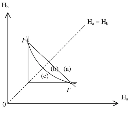
The parameter r measures the degree of aversion to inequality, as represented by the
convexity of the iso-welfare curves. If r = -1, social welfare is equal to the sum of
individual health and there is no aversion to inequality. This utilitarian-type SWF
results in iso-welfare contours that are parallel straight lines with a gradient of -1, as
shown by curve (a) in Figure 1. If r > -1, there is aversion to inequality, as represented
by a diminishing MRS between the health of the two groups; that is, along a given
iso-welfare curve, the greater the inequalities in health between the two groups, the greater
is the weight given to the worse-off group relative to the better-off group. This results
in iso-welfare curves that are convex to the origin, as shown by curve (b) in Figure 1. In
the extreme, r approaches ∞ and all that matters is the health of the worse-off group.
This results in a Rawlsian-type SWF with right-angled iso-welfare curves, as shown by
curve (c) in Figure 1.
III. ESTIMATING THE SHAPE OF THE SWF
The question now is how do we measure the value of r? One approach would be to
retrospectively collect information on existing public polices and, on the assumption
that government decision-making is rational, regress the data to estimate values for the
parameters. An alternative approach, which is the one adopted here, is to elicit the
preferences of the general public over stylised questions specifically designed to allow
us to estimate the values of r (see Amiel and Cowell 1999 for more discussion of the
9
Williams (1997) suggests that respondents could be presented with the current unequal
distribution of health and then asked to think about an equal distribution of health that
makes them indifferent between the two distributions. In this way, the general format of
the questions would be similar to those used by Amiel and Cowell (1999), and by Amiel
et al (1999) in their “leaky-bucket experiments”. However, whilst it is possible to take
income from one person and transfer it to another, it is not possible to redistribute health
in the same way. Moreover, if individuals evaluate outcomes as gains or losses relative
to some perceived reference point, and if losses are weighted more heavily than gains
(see Kahneman and Tversky 1984), then this will confound the calculation of the
implied equity-efficiency trade-off. Therefore, it seems more appropriate to calculate
the value of r by considering the distribution of gains in health from an initial position.
Figure 2 shows the basic format of the questions in relation to the SWF. The initial
situation (I) is presented to respondents together with a programme (A) that will benefit
both groups by the same amount. They are then presented with an alternative
programme (B) that targets the benefit on the worse-off group. The aim then is to
determine, in an iterative way, how much programme B would have to benefit the
worse-off group in order to be considered equally as valuable as programme A. Once
indifference between programmes A and B has been established, the value of r can be
calculated. From this, the weight given to a unit health gain to the worse-off group
10
More formally, if Ha(B) stands for the value of health of subgroup a (who are assumed
to be less advantaged at the initial point) at point B, then the corresponding gradient at
the midpoint of A and B is:
( )
(
)
(
)
( )r
a a b b r a b a b B H A H B H A H H H dH
dH + +
+ + − = − = 1 1 2 ) ( ) ( 2 ) ( ) (
. [2]
Furthermore, by definition, the same gradient can be approximated as:
) ( ) ( ) ( ) ( A H B H A H B H dH dH a a b b a b − −
≈ . [3]
Therefore, by taking the logarithms of these and by solving this, a unique value of r
(which is independent of the initial point) can be obtained:
(
) (
)
(
)
(
) (
)
(
( ) ( ) ( ) ( ))
1log ) ( ) ( ) ( ) ( log − + + − − ≈ B H A H B H A H A H B H B H A H r a a b b a a b b
. [4]
The weight implied to the less advantaged group a relative to group b is calculated from
the marginal rate of substitution:
) 1 ( r a b a b H H dH dH + =
− . [5]
Notice that the value of r increases exponentially with the extent of the
11
mean of any group of values would give greater relative weight to the preferences of
those most concerned about equity. This makes it difficult to account for the strength of
each individual’s preferences in the overall preferences of a group. For this reason, we
will concentrate our analysis and interpretation on the median. Use of the median is
also consistent with the median voter rule, which has been used to model public policy
choices (Mueller 1979).
Any one respondent could be asked to adopt a number of different perspectives when
answering questions of the kind shown in Figure 2. For example, she could be asked to
think of herself as: 1) a member of the better off or worse off group; 2) facing a known
or unknown probability of being in each of those groups; or 3) not being in either group.
Some economists would argue that the first, personal perspective does not adequately
detach individuals from their own self-interest (Harsanyi 1982) and others would argue
that the third, citizen-type perspective is unsuitable since it ignores self-interest
completely (Johannesson 1999). This would leave the second perspective as the only
appropriate one. According to this view, the operational device of a veil of ignorance
should be used since it detaches the individual from her own vested interest by
concealing her position in society, but still asks her to consider allocation decisions on
the basis that she herself will ultimately be affected by them (Rawls 1972).
However, the use of the veil of ignorance to determine a just distribution is hotly
contested. Dworkin (1977) is highly critical of the hypothetical nature of the contract that
people are asked to enter into. Barry (1989) questions the link that is made between
individual preferences from behind the veil with a just society once the veil has been
12
impartiality, it is not enough to explain why people’s preferences about gambles should
provide any reason to favour one social situation rather than another (but see also
Harsanyi (1982) for an opposing view).
For these reasons, it was decided not to use the veil of ignorance in this study. Instead,
we asked respondents to adopt a citizen’s perspective, rather like the one adopted by
Amiel and Cowell (1999) in their empirical studies on income inequalities. To us, and
as famously emphasised by Rousseau (1762), there is legitimate distinction between a
person’s self-regarding preferences based on her own self-interest and her
society-regarding preferences which reflect her views about what society should look like. The
distinction has more recently received attention – and support – from a number of
economists and political scientists, including Harsanyi (1955) and Etzioni(1986). We
therefore collected information on a range of background characteristics in order to
examine the extent to which self-interest might be playing a part in responses.
IV. THE EMPIRICAL STUDY
Differences in health in this study, as noted in section 2, have been defined in terms of
average life expectancy and rates of limiting long-term illness. People are familiar with
these representations of health and they provide us with the opportunity to test whether
the SWF has a different shape depending on how health is represented. The question
that remains is which groups are these differences to be defined across? The most
obvious differences in health in the UK exist between the social classes (Acheson
1998). Of the six social classes often used in British surveys, we employ data
13
lowest social classes highlights the extent of the prevailing inequalities and has the
advantage that the fraction of the population in each of these classes is roughly the same
(about 7% in each case).
One of the questions we asked concerns difference in life expectancy at birth. On
average, people in the highest social class (such as doctors and other professionals) live
five years longer than those in the lowest social class (unskilled manual workers such as
cleaners). Another question is about prevalence of limiting long-term illnesses. For
males aged 45-64, 12% of those in the highest social class report limiting long-term
illness compared to 40% of those in the lowest social class.
Furthermore, population subgroups other than social class were also used. Differences
of the same magnitude (5 years) in average life expectancy exist between women and
men. This means that by presenting other respondents with identical questions
regarding life expectancy, but relating them to differences by sex instead of by social
class, it is possible to test whether the value of r is a function of the groups across which
the inequalities exist. To further test the sensitivity of r, other respondents were
presented with the same life expectancy and long-term illness differences across groups
that were simply defined as the ‘healthiest 20%’ and the ‘unhealthiest 20%’ of the
population.
The questionnaire was administered during a face-to-face interview, which gave the
interviewer the opportunity to assess the respondent’s understanding of the task and
provided the respondent with the opportunity to ask any clarificatory questions. The
14
sub-groups used. The questionnaire was developed through in-depth interviews and
extensive piloting, during which time it emerged that the clearest way in which to
represent the health of the two groups was in the form of graphical representations, as
shown in the appendix. For each of the life expectancy and long-term illness questions,
respondents were first asked to make a discrete choice between Programme A (that
benefits both groups by the same amount) and Programme B (that targets the same
amount of overall benefit on the worse-off group). They were told that the two groups
were of approximately equal size and that the two programmes would cost the same.
For those respondents who chose programme A, it was assumed that, since they were
unwilling to target the worse off group when overall benefits were the same, they would
also be unwilling to target the worse off group when overall benefits were reduced, and
so no further sub-questions were asked. Those respondents who chose programme B
were presented with a series of pairwise choices in which the benefits from choosing B
were gradually reduced. This order was chosen to make the trade-off between
efficiency and equity as transparent as possible and because it was felt that it would be
cognitively less demanding for respondents than a random order that would have
required them to ‘jump around’ between different trade-offs. Note that respondents
were not provided with the opportunity to state that they were indifferent between the
two programmes. This option was in the pilot interviews but was never chosen and in
fact caused confusion.
The interviews were carried out in two rounds. The response categories presented in the
two rounds are shown in Tables 1 and 2. Differences in health by sex were used in the
15
second round. Social class differences were also used in both rounds to allow for direct
comparisons across the two rounds. Respondents in the first round who initially chose
programme B were presented with six additional pairwise choices. The response
categories in the second round of interviews were revised in the light of the distribution
of responses from the first round, resulting in only four additional pairwise choices in
the second round. In addition to some of the response categories in the first round being
largely redundant, this allowed us to test whether respondents were following a
particular pattern of responses e.g. choosing the middle option.
In order to interview a broadly representative sample of the general population, every
8th person on the electoral register in three wards in York was contacted and invited to
participate, for which they would receive £15. Out of a total of 1,500 letters of
invitation, 467 people (31%) agreed to take part. To ensure representativeness, 140
respondents were selected for interview based on information on a broad range of
characteristics obtained from their reply slips. In total, 130 individuals were
interviewed by one of the authors and two other researchers. The interviews took place
at the University of York and lasted for about an hour, of which the first fifteen minutes
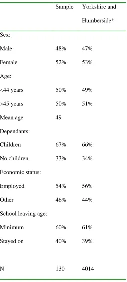
were spent on the questions analysed in this paper. Table 3 shows the characteristics of
the sample, and confirms that the characteristics of those who attended the interviews
were similar to those of the population of the Yorkshire and Humberside region.
V. CALCULATING THE SWF
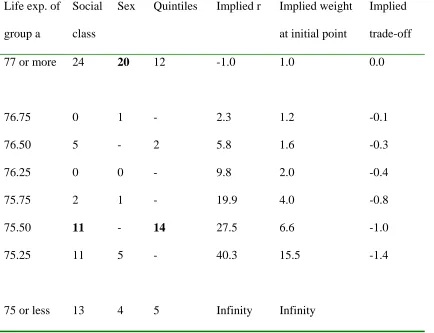
The results from the empirical study are summarised in Tables 4 and 5. For those
16
point to programme A, their point of indifference has been taken to be half-way
between the last point at which they chose B and the first point at which they chose A.
The precise trade-offs made by those who choose not to target and by those who always
choose to target are indeterminate, and so, strictly speaking, r can only be calculated for
those respondents who switch from programme B to programme A at some point. For
those who chose A in the initial pairwise comparison, we have assumed that r = -1
although we cannot rule out the possibility that some respondents may have favoured
increased inequality. For those who always chose B, we have assumed that they are
concerned only with equality and hence r approaches ∞, but again we cannot be sure.
Columns 2-4 in Table 4 present the distribution of responses in the context of average
life expectancy. Since the implied trade-offs that respondents made between the social
classes did not differ across the rounds (Mann Whitney U Test, p>0.05), the responses
from both rounds have been pooled. The median respondent is indifferent between
people in the highest and lowest social classes living on average to be 80 and 75,
respectively, and these groups living to be 78 and 75.5, respectively. This is also the
median response when the sub-groups are defined in terms of the healthiest and
unhealthiest quintiles of the population. However, when identical data are presented but
the sub-groups are defined by sex, the median preference is to favour no targeting of
men at all.
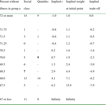
Columns 2 and 3 in Table 5 show the results from the long-term illness question. The
median respondent is indifferent between a decrease in the rate of long-term illness of
7% for both groups and a 2% and 8% reduction when the groups are defined by social
17
and unhealthiest quintiles. These responses are not statistically significantly different
from one another (Mann Whitney U Test, p>0.05). The responses in Tables 4 and 5
were not related to any of the personal characteristics shown in Table 3 (using the χ2
test, p>0.05).
The 5th column in Table 4 and the 4th column in Table 5 represent the implied value of
the r parameter for all question options. Notice that the value of r is independent of the
level of health at the initial point (see equation [4]). The implied weights at the initial
point for each of the question options are given in the 6th and 5th columns of Tables 4
and 5, respectively. For example, at the initial point, a given gain in life expectancy to
the lowest social class is, according to the median respondent, weighted about seven
times as highly as an equivalent gain to the highest social class, whereas a given
reduction in long-term illness is weighted about four times as highly.
The final columns of both tables show the implied equity-efficiency trade-offs in terms
of health at the initial point. The concept is borrowed from the literature on income
inequalities and is calculated here as the difference between average health and the
“equally-distributed equivalent health”. The latter represents the level of overall
population health that, if distributed equally across the population, is as good as a given
unequal distribution. The negative values in these columns indicate the losses in
efficiency people are willing to forego for equality between the two groups. So, in the
case of average life expectancy by social class in Table 4, the median respondent would
be indifferent between the initial point (where the highest and lowest social classes live
18
they would be willing to trade-off up to one year of the average health of these two
19
VI. DISCUSSION
This study has sought to determine the shape of a health-related SWF from people’s
stated preferences over various equity-efficiency trade-offs. It indicates that it is
possible to ask people to make meaningful quantitative trade-offs between efficiency
and equity. The results are consistent and plausible, and suggest that preferences are
sensitive to the type of health inequalities that exist and to the groups across which the
inequalities exist. We are able to conclude that in this domain it is possible to specify a
SWF that is useful for very concrete policy purposes.
The study nevertheless raises a number of issues that warrant further discussion. The
questions were designed to present respondents with equity-efficiency trade-offs in
policy-relevant and unambiguous terms, and in a manner that makes measurement
possible. In the first part of each question, the information regarding the size of the
health gains of the two programmes was easy to understand and, in the second part of
each question, the implications of choices were made clear through changes in the size
of the bars on the graph. However, to facilitate this visual representation, the scales on
the graphs in the life expectancy question did not start at zero (see the appendix), and
this could have led some respondents to perceive that the relative difference between the
two groups was larger than it really was.
In general, it has been shown that very subtle changes in the framing of a question can
sometimes have a dramatic effect on responses (for an excellent review, see Rabin
1998). This study was designed to minimise the effects of certain framing effects but it
20
evidence from other studies that suggests that respondents might be reluctant to give all
the benefit to one individual or group (see, for example, Cuadras-Morato et al 2001).
And so in our question about life expectancy (in which the targeted programme gives no
benefit to the better-off group), it is encouraging that more people wish to target the
lowest social class in this question than in the question about long-term illness (in which
the targeted programme is of some benefit to the better-off group). We went further,
though, and asked respondents who chose not to target in the life expectancy question if
they would have targeted if there had instead been a one-year benefit to the better-off
group (and hence a three-year benefit to the worse-off group). None of these
respondents chose to revise their answers.
There are also reasons for supposing that respondents might have been more inclined to
choose programme A in both questions. It is now well established that respondents may
give greater weight to the losses of one group as compared to an equivalent gain to the
other group (Schweitzer 1995). Therefore, the questions were designed so that neither
programme in the two questions involved any losses, and so that neither programme
was presented as representing the status quo. It is possible that loss aversion may also
be present when considering potential as well as actual losses from a particular
reference point (Dolan and Robinson 2001). Therefore, if some respondents adopted
the potential gains available to both groups in programme A as their reference point,
then programme B would involve a ‘loss’ to the better-off group. It would be
interesting, and policy relevant, to test with further research how sensitive the degree of
21
There is a status quo bias of a different kind that might have made respondents more
inclined to stick with programme B if they chose it initially. This relates to the fact that
respondents were always presented with response categories in the same order; that is,
programmes A and B start out being equally effective and then B becomes
incrementally less effective. This ordering was chosen to make the equity-efficiency
trade-off as transparent as possible and was informed by the results from the pilot
interviews which suggested that the trade-off questions would have been cognitively too
difficult if the ordering of the response categories was randomised. However, there is
the possibility of a status quo bias whereby some respondents get ‘locked into’ choosing
B throughout (see Samuelsen and Zeckhauser 1988). Whilst we cannot rule out the fact
that this ordering might have induced some respondents to choose programme B more
often, many did eventually switch to programme A, suggesting that they became aware
at some point of the loss in efficiency from continuing to choose B.
There are also general questions relating to the reliability of stated preference data,
particularly of the kind gathered in this study, which asked respondents to consider their
preferences over benefits to other people. As with other studies that have sought to
elicit citizen-type preferences over different public policies, it is not possible to test our
results against the preferences that respondents reveal in their private consumer-type
behaviour. Economists are certainly brought up to believe that preferences that are not
motivated by any degree of self-interest cannot be trusted, but this scepticism follows
from the assumption that social welfare is primarily a function of the utility levels of
self-interested individuals. This is certainly contestable since, although self-interest exists, it
does not necessarily follow that it must be the basis for social welfare calculations since
22
A related criticism of studies of this kind, which use face-to-face interviews, is that
some respondents may have given what Miller (1992) refers to as ‘Sunday Best’
responses; that is, “the views that people think they ought to hold according to some
imbibed theory as opposed to the operational beliefs that would guide them in a
practical situation.” We certainly cannot dismiss this possibility but many people did
not wish to target (including over one-third of respondents in the life expectancy by
social class question), so evidence of it is weak. In any event, there is an argument that
only those preferences and social values that people are prepared to air publicly should
be used to inform social policies which are designed to incorporate the public’s views
on social justice (Gauthier 1986).
Despite concerns such as these, we believe that this study represents a distinct advance
in terms of both the methodology used and usefulness for policy purposes. It suggests
that differences in average life expectancy could be more important to people than
differences in rates of long-term illness. Another particularly striking result is that
differences in the average life expectancies of men and women did not seem to matter
much at all, with the median respondent unwilling to sacrifice any overall gains in life
expectancy in order to target men. Future research might try to get behind some of the
reasons for the very different attitudes towards health inequalities by sex as compared to
those by social class.
In conclusion, this study has demonstrated that, using carefully designed questionnaire
instruments, the SWF can develop from being a theoretical construct to becoming a
23
meaningful trade-off responses from the general population that can then be used to
determine the shape of the SWF. We therefore believe that the study indicates a
promising new avenue of economic enquiry that is highly relevant to important public
24
ACKNOWLEDGEMENTS
We would like to thank John Cairns, Atsushi Higuchi, Peter Lambert, Chris McCabe
and Jan Abel Olsen for their helpful comments. The paper has also benefited from the
comments made by participants at seminars at the Universities of East Anglia and Oslo.
We are grateful to all the respondents who agreed to take part. Rebecca Shaw was
supported by the Economic and Social Research Council (Award No: L128251050).
25
REFERENCES
AMIEL, Y. and COWELL, F.A. (1999). Thinking about Inequality. Cambridge:
Cambridge University Press.
AMIEL, Y., CREEDY, J. and HURN, S. (1999). Measuring attitudes towards
inequality. Scandinavian Journal of Economics, 101(1), 83-96.
ATKINSON, A.B. (1970). On the measurement of inequality. Journal of Economic
Theory, 2, 244-263.
BARRY, B.M. (1989) A treatise on social justice, vol I: Theories of justice. University
of California Press.
BOADWAY, R. and BRUCE, N. (1984). Welfare Economics. Basil Blackwell
BROOME, J. (1991). Weighing Goods. Basil Blackwell.
CUADRAS-MORATO, X., PINTO-PRADES, J.L. and ABELLAN-PERPINAN, J.M.
(2001).’Equity considerations in health care: the relevance of claims, Health
Economics, 10(3),187-205.
CULYER, A J. (1989). The normative economics of health care finance and provision.
26
DOLAN, P. (1998). The measurement of individual utility and social welfare. Journal
of Health Economics, 17, 39-52.
DOLAN, P. and ROBINSON, A. (2001). The measurement of preferences over the
distribution of benefits: the importance of reference points. European Economic Review,
45(9), 1697-1709.
DWORKIN, R. (1977). Taking rights seriously, Duckworth
ETZIONI, A. (1986). The case for a multiple utility conception, Economics and
Philosophy, 159-183.
GAUTHIER, D. (1986). Morals by agreement. Oxford: Oxford University Press.
HARSANYI, J. (1955). Cardinal welfare, individualistic ethics and interpersonal
comparisons of utility, Journal of Political Economy, 63, 309-321.
HARSANYI, J.C. (1982). Morality and the theory of rational behaviour. In Sen, A. and
Williams, B. (eds.) Utilitarianism and Beyond, Cambridge University Press.
Independent Inquiry into Inequalities in Health. (1998). Independent Inquiry into
Inequalities in Health Report (The Acheson Report). London: The Stationary Office.
JOHANNESSON, M. (1999). On aggregating QALYs: a comment on Dolan. Journal of
27
KAHNEMANN, D. and TVERSKY, A. (1984). Choices values and frames, American
Psychologist, 39, 341-350.
LAYARD, R. and WALTERS, A.A. (1994). Allowing for income distribution. In
Laylard, R. and Glasiter, S. (eds.), Cost-Benefit Analysis (2nd ed.,): Cambridge
University Press (reprinted from Layard, R. and Walters, A. A. 1978. Microeconomic
Theory, McGraw-Hill)
LITTLE, I.M.D. and MIRRLEES, J.A. (1974). Project appraisal and planning for
developing countries: Heinemann Educational Books.
MUELLER, D. (1979). Public Choice, Cambridge University Press.
MUSGRAVE, R.A. (1959). The Theory of Public Finance, McGraw Hill.
MENZEL, P. (1999). How should what economists call ‘social values’ be measured?
The Journal of Ethics, 3, 249-273.
MILLER, D. (1992). Distributive justice: what do people think? Ethics, 102, 555-593.
OLSEN, J A. (1997). Theories of justice and their implications for priority setting in
28
RABIN, M. (1998). Psychology and economics. Journal of Economic Literature, 36,
11-46.
RAWLS, J. (1971). A Theory of Justice, Oxford University Press.
ROUSSEAU, J.J. (1762).The Social Contract, (1998 translation) London:Wordsworth
SAMUELSON, W. and ZECKHAUSER, R. (1988). Status quo bias in
decision-making, Journal of Risk and Uncertainty, 1: 7-59
SCANLON, T.M. (1975), Preference and urgency, Journal of Philosophy, 72, 655-669
SEN, A. (1992). Inequality reexamined. Oxford University Press.
SCHWEITZER, M. (1995). Multiple reference points, framing, and the status-quo bias
in health-care financing decisions, Organizational Behavior and Human Decision
Processes, 63, 69-72.
WILLIAMS, A. (1997). Intergenerational equity: an exploration of the 'fair innings'
29
Figure 1: The effect of changes in the value of r
Hb
Ha = Hb
I
(a) (b) (c)
I'
0
Ha
Ha, Hb: health of sub-populations a and b I: the initial state
I': the point where the health levels of the two groups are exchanged It is assumed that α = β
Three different types of social welfare contours: (a): r = -1 … cf. the classical utilitarian
30
Ha: health of the less advantaged group
Hb: health of the more advantaged group
I: initial point
It is assumed that α = β
A: outcome offered by programme A
the horizontal broken line: the set of options (1 to n) offered by the alternative programme B
B: the point at which the median respondent is indifferent between the two programmes, and thus the point through which the iso-welfare curve crosses the broken line
Figure 2: The SWF and the life expectancy questions
Hb
A Ha = Hb
n .… B …1 I
iso-welfare
31
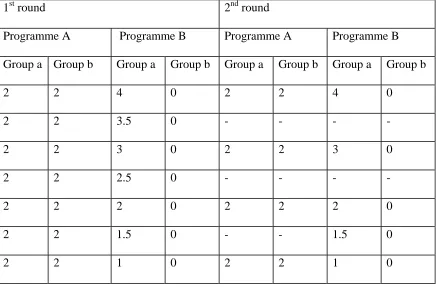
Table 1: Life expectancy response options
The initial situation is one in which group a (the worst-off group) live to be 73 and
group b (the best-off group) live to be 78. The numbers in the table show average
increases in life expectancy per group for each of the pairwise choices.
1st round 2nd round
Programme A Programme B Programme A Programme B
Group a Group b Group a Group b Group a Group b Group a Group b
2 2 4 0 2 2 4 0
2 2 3.5 0 - - - -
2 2 3 0 2 2 3 0
2 2 2.5 0 - - - -
2 2 2 0 2 2 2 0
2 2 1.5 0 - - 1.5 0
2 2 1 0 2 2 1 0
32
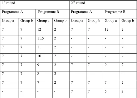
Table 2: Long-term illness response options
The initial situation is one in which group a (the worst-off group) have a rate of limiting
long-term illness of 40% and group b (the best-off group) have a corresponding rate of
12%. The numbers in the table show percentage reductions in the absolute rate per
group depending on the programme chosen for each of the pairwise choices.
1st round 2nd round
Programme A Programme B Programme A Programme B
Group a Group b Group a Group b Group a Group b Group a Group b
7 7 12 2 7 7 12 2
7 7 11.5 2 - - - -
7 7 11 2 - - - -
7 7 10 2 - - - -
7 7 9 2 7 7 9 2
7 7 8 2 - - - -
7 7 7 2 7 7 7 2
- - - - 7 7 5 2
33
Table 3: Respondent characteristics
Sample Yorkshire and
Humberside*
Sex:
Male 48% 47%
Female 52% 53%
Age:
<44 years 50% 49%
>45 years 50% 51%
Mean age 49
Dependants:
Children 67% 66%
No children 33% 34%
Economic status:
Employed 54% 56%
Other 46% 44%
School leaving age:
Minimum 60% 61%
Stayed on 40% 39%
N 130 4014
* The Annual Survey of English Housing 1998/1999 and The British Household
34
Table 4: Average life expectancy questions
Life exp. of
group a
Social
class
Sex Quintiles Implied r Implied weight
at initial point
Implied
trade-off
77 or more 24 20 12 -1.0 1.0 0.0
76.75 0 1 - 2.3 1.2 -0.1
76.50 5 - 2 5.8 1.6 -0.3
76.25 0 0 - 9.8 2.0 -0.4
75.75 2 1 - 19.9 4.0 -0.8
75.50 11 - 14 27.5 6.6 -1.0
75.25 11 5 - 40.3 15.5 -1.4
75 or less 13 4 5 Infinity Infinity
Median respondent in bold
35
Table 5: Limiting long-term illness questions
Percent without
illness in group a
Social
class
Quintiles Implied r Implied weight
at initial point
Implied
trade-off
72 or more 14 9 -1.0 1.0 0.0
71.75 1 - -0.8 1.1 -0.2
71.5 3 1 -0.6 1.1 -0.5
71.25 0 - -0.4 1.2 -0.7
70.5 1 - 0.2 1.6 -1.6
70.0 5 9 0.7 1.9 -2.3
69.5 6 - 1.3 2.4 -3.0
68.5 7 - 2.9 4.4 -4.9
68.0 13 14 4.1 7.1 -6.2
67.5 5 - 6.2 15.9 -7.9
67 or less 11 0 Infinity Infinity
Median respondent in bold
36
Appendix: Example of the questions – average life expectancy by social class
As you might know, average life expectancy differs by social class.
Whilst actual life expectancy varies between individuals, on average, people in social class 1 live to be 78 and in social class 5 they live to be 73.
Imagine that you are asked to choose between two programmes which will increase average life expectancy. Both programmes cost the same.
In the two graphs below the light grey part shows average life expectancy, and the dark grey part shows the increase in life expectancy. There is a separate graph for each of the programmes.
As you can see, Programme A is aimed at both social classes equally and Programme B is aimed more at social class 5.
Please indicate whether you would choose A or B by ticking one box.
Programme A Programme B
Class I Class V Class I Class V
If the respondent chose A, that was the end of the question. If the respondent chose B, she was told:
“Choosing Programme B might mean that the increase in life expectancy is less overall. For each of the six [or four, depending on the round] choices below, please tick one box to indicate whether you would still choose B, or whether you would now choose A.”
The presentation of the choices was of the same kind as that illustrated above
68 68