Thesis submitted in accordance with the requirements of the University of Liverpool for the degree of Doctor in Philosophy
by
Mohammed Ibrahim Mohammed Mustafa
200573203
Oliver Lodge Laboratory
• The pure soul of my deceased father, God forgive him who, after God, was the source of guidance and support to me throughout my life.
• The soure of inspiration my mother, for all her sufferings and endurance that she faced throughout her life to educate me in the best way.
• My sisters and brothers who have given me the opportunity to maintain my professional development and have undertaken all my study costs in different stages of my life.
I would like to take this opportunity to express my deepest appreciation and thanks to thsoe people who guided me and shared their experiences during my four years study and research. Without their guidance and persistent assistance, this thesis would not have been possible.
• I would like to thank, foremost my supervisor Prof. Paul Nolan, for allowing me the opportunity to study at thr University of Liverpool, who was the source of ongoing guidance and support during my time as a PhD student.
• I would like also to thank the well-known and highly respected experts in the nu-clear structure of Erbium nuclei, Prof. John Simpson with Dr. Eddie Paul and Dr. James Ollier for their insights on my research analysis through responses to all the questions that I have during my research.
• A special thanks to my secondary supervisour Dr Andy Boston, with Prof. Rodi Herzberg, Prof. Robert Page and Dr. Dave Joss for giving me the opportunity to take a part in all MSc. and postgraduate modules during my first year.
• In addition, I would like to thank all PhD students of the Liverpool Nuclear Structure Group, both past and present, especially John Revill, Robert Carroll, Laim Gaffney and Joseph Ress for their assistance to training practice tech-niques that have been used in this research and for proof reading this thesis.
• I express my gratitude to that relative justice which is verified in higher educa-tion in Iraq after freedom day (09/04/2003), that gave an opportunity for me and thousands of iraqi students to complete postgraduate study.
In the current work a detailed spectroscopic investigations of the gamma-decays from the excited states of the rare-earth nucleus 159Er has been performed to study the
structural properties up to possible ultrahigh spins. The nucleus of 159Er had been
populated by the reaction116Cd(48Ca,5nγ) at beam energy of 215-MeV in an
Contents . . . i
1 Introduction 1 1.1 Introduction . . . 1
2 Nuclear Models 3 2.1 Introduction . . . 3
2.2 The Nuclear Shell Model . . . 4
2.3 Spherical Shell Model and Nuclear Potential . . . 5
2.3.1 Harmonic Oscillator Potential . . . 6
2.3.2 Spin Orbit Interaction . . . 8
2.3.3 Woods-Saxon Potential . . . 10
2.4 Nuclear Deformation . . . 10
2.5 The Anisotropic Harmonic Oscillator Potential . . . 12
2.6 Nilsson Model . . . 14
2.7 The Strutinsky Shell Correction Procedure . . . 17
2.8 Pairing and Quasiparticles . . . 18
3 Nuclear Rotation 21 3.1 Introduction . . . 21
3.2 Non-Collective Single Particle Excitation . . . 21
3.3 Collective Excitation . . . 22
3.4 Rotational Frequency and Moment of Inertia . . . 24
3.7 Nuclear Symmetries . . . 28
3.7.1 Parity . . . 29
3.7.2 Signature . . . 29
4 Experimental Details 31 4.1 Introduction . . . 31
4.2 Heavy Ion Fusion Evaporation Reaction . . . 31
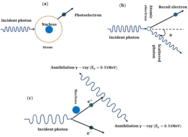
4.3 Gamma-ray Interaction Processes with Matter: . . . 35
4.3.1 Photoelectric Absorption . . . 35
4.3.2 Compton Scattering . . . 36
4.3.3 Pair Production . . . 37
4.4 Gamma-ray Detectors . . . 37
4.4.1 Scintillation Detectors . . . 38
4.4.2 High-Purity Germanium (HPGe) Detectors . . . 38
4.4.3 Compton Suppressed Germanium Detector . . . 40
4.5 Gammasphere Array . . . 41
4.6 The Experimental Details . . . 42
4.7 Data Analysis . . . 44
4.7.1 Hypercube Analysis . . . 44
4.7.2 Angular Intensity Ratio Measurment . . . 45
4.8 Gamma Decay . . . 46
5 159Er Results 47 5.1 Introduction . . . 47
5.2 Motivation . . . 47
5.3 159Er Results . . . . 48
5.4 High Spin Structure . . . 49
5.4.1 Yrast Band (+, +1/2) . . . 49
5.4.4 Band 3 (−, −1/2) . . . 61
5.4.5 Band 4 (−, +1/2) . . . 65
5.4.6 Band 5 (−, +1/2) . . . 69
5.4.7 Band 10 (−,−1/2) . . . 70
5.4.8 TSD 1 (−, +1/2) . . . 71
5.4.9 Gamma Vibrational Band (+, +1/2) . . . 73
5.5 Strongly Coupled High K Structures . . . 75
5.5.1 Strongly Coupled Bands 6 and 7 . . . 75
5.5.2 Strongly Coupled Bands 8 and 9 . . . 80
6 Interpretation of Structure of 159Er 90 6.1 Introduction . . . 90
6.2 Alignment and Rotational Properties of the Bands . . . 91
6.3 Cranked Shell Model . . . 92
6.4 Cranked Nilsson-Strutinsky Calculation (CNS) . . . 95
6.5 Positive Parity Bands: . . . 99
6.5.1 Yrast Band . . . 99
6.5.2 Band 1 . . . 105
6.5.3 Gamma-Band . . . 106
6.6 Negative Parity Bands: . . . 108
6.6.1 Band 2 . . . 108
6.6.2 Band 3 . . . 112
6.6.3 Band 4 . . . 113
6.6.4 Band 5 . . . 114
6.6.5 Band 10 . . . 116
6.7 Strongly Coupled Structure Bands: . . . 116
6.7.1 Bands 6 and 7 . . . 119
6.7.2 Bands 8 and 9 . . . 121
2.1 An illustration of three potential wells used to model the nuclear po-tential. V0 is the well depth, r the distance from the origin, and ro the
nuclear radius. . . 6 2.2 Single particle energy levels of the harmonic oscillator potential with
the effects ofl2 term and spin-orbit interaction. . . . 9
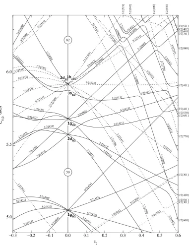
2.3 The Lund convention for the quadrupole deformation shapes in nuclei. 11 2.4 Illustration of the labelling of orbitals in the Nilsson model. . . 13 2.5 Nilsson diagram of single-neutron energies (50 < N <82) as a function
of the quadrupole deformation parameter ε2. Full and dashed lines
correspond to positive and negative parity respectively. . . 15 2.6 Nilsson diagram of single-proton energies (50< N < 82) as a function
of the quadrupole deformation parameter ε2. Full and dashed lines
correspond to positive and negative parity respectively . . . 16 2.7 The left figure illustrates a pair of nucleons in time reversed orbital
(a), scattered into another time reversed orbital (b). The figure on the right side illustrates the single particle occupation probability as a function of single particle energy and explains the effect of pairing correltion on the Fermi surface. . . 19
3.1 Illustrates rotation of an axial symmetric nucleus around an axis per-pendicular to the symmetry axis, and its angular momenta projections. 22
excitation. (b) Collective rotation in a deformed nucleus to generate angular momentum collectively and exhibit a rotational band in 158Er. 23
3.3 Particle rotor coupling scheme (a) Deformation aligned and (b) Rota-tional alignment. . . 26 3.4 Illustration of the effects of cranking on the remaining symmetries that
describe a particular configuration of nucleons. . . 28
4.1 Schematic illustration of the dependance of angular momentum of the nuclear excited system on the impact parameter (b) and the separation distance (R) between the centres of colliding nuclei. . . 33 4.2 Various stages with time scales of the heavy ion fusion evaporation
reaction for product nucleus 159Er. . . . 33
4.3 Schematic illustation of the de-excitation modes of highly excited com-pound nucleus. . . 34 4.4 Schematic illustation for the interction processes of gamma-ray with
matter, (a) photoelectric absorsorption, (b) Compton scattering and (c) pair production. . . 36 4.5 Gamma-ray spectra for 1.173 MeV and 1.332 MeV of 60Co source
ob-tained by using the HPGe detector used in the Gammasphere array, with Compton suppressed shield and without suppressed shield. . . . 39 4.6 Schematic illustation of Compton-suppressed HPGe detecter used in
the Gammasphere array. . . 40 4.7 The Gammasphere array at Argonne National Laboratory. . . 42
given in keV, and the width of the arrows indicate the relative inten-sities of the transitions. Beneath each band in italics, the bandhead energy is given in keV. Spins and parities are based on measurements of angular intensity-ratios, and parenthesis indicate tentative spin and parity assigments. Where the observation of a transition is considered tentative, a dashed arrow and parenthesis are used. . . 50 5.2 Partial level scheme for 159Er constructed from the present work for
negative parity high-spin band structures. The transition energies are given in keV, and the width of the arrows indicate the relative inten-sities of the transitions. Beneath each band in italics, the bandhead energy is given in keV. Spins and parities are based on measurements of angular intensity-ratios, and parenthesis indicate tentative spin and parity assigments. Where the observation of a transition is considered tentative, a dashed arrow and parenthesis are used. . . 51 5.3 Angular intensity-ratios, R, for gamma-rays as a function of transition
energy for the previously observed bands; Yrast, Band 1, Band 2, Band 3 and Band 4 in159Er. . . . 52
5.4 Angular intensity-ratios, R, for gamma-rays as a function of transition energy for new bands; Gamma-Band, Band 5 and Band 10 in159Er. . 52
101/2 and 105/2 states. Linking transitions above the 85/2 state are marked blue, and transitions in the parallel sequence are marked red. The coincidence spectrum (b) verifies that the initial state of the 941-keV transition is depopulated from the fully aligned terminating 101/2+ state. Spectra (a) and (c) provide the evidence for re-ordering
the transitions in the yrast band shown in the level scheme of Figure (5.1). The spectra were produced from varoius sum of triple gates set on yrast transitions; (a) from 208-keV to 1096-keV, and (b) from 830-keV to the 1153/1154-keV transitions in coincidence with the 1342-keV, and (c) from 830-keV to the 1232-keV except the 1153/1154-keV transitions in coincidence with the 1276-keV transition. . . 54 5.6 Coincidence spectrum produced from a sum of triple gates set on
tran-sitions from 208-keV to 1096-keV in the yrast band of 159Er. . . . 56
5.7 Coincidence spectra showing transitions from the decay of states in the Band 1 of 159Er. (a) is produced with a sum of double gates set on
transitions from the decay of the 55/2+ state to (67/2+) state in Band
1, marked with asterisks, and clearly shows the 1008-keV transition which has initial state 91/2+. Coincidence spectrum in (b) is produced
with a sum of triple gates set on in-band transitions from the 228-keV to 1105 keV in Band 1, which shows all transitions coincidence with Band 1. The linking transitions are marked in green, and clearly shows transition of 1008-keV depopulated from state 91/2+. . . . 57
duced with a sum of triple gates set on coincidence transitions from the decay of the 53/2+ state to (93/2+) state marked with asterisks and
1208-keV. (b) Transitions above the state 49/2− in coincidence with the 1188-keV, produced with a sum of triple gates set on coincidence transitions from the decay of the 53/2+ state to (93/2+) state marked
with asterisks and 1292-keV. (c) Produced with a sum of triple gets set on all in-band transitions up to the (97/2−) state in Band 2, which shows all transitions coincidence with Band 1. The linking transitions are marked in green. . . 60 5.9 Coincidence spectra from the decay of states in the Band 3 of 159Er.
Spectrum in (a) shows the three new transitions of 403-keV, 410-keV and 490-keV in coincidence with the previously observed transitions, produced with a sum of triple gates set on transtions marked with c, 145-keV, 284-keV and 403-keV in coincidence with the transitions marked with d, 485-keV, 588-keV and 687-keV. Spectrum in (b) dis-plays the majority of transitions in Band 3 in coincidence with the most intense transitions of the yrast band. Produced with a sum of triple gates on in-band transitions from the decay of the 31/2+ state
to 83/2+ state. In the specta, linking transitions are marked in green
and transitions of the yrast band in blue. . . 63
set on the coincidence transitions from the decay of the 39/2− state to the 79/2− state in coincidence with 1209-keV transition, and in (b) is produced from a sum of the same triple gate in coincidence with 1222-keV transition. In the specta, the transitions that are linking band 3 to the yrast band marked in red, and a yrast transition of 625-keV is marked in in blue. . . 64 5.11 Coincidence spectra produced with a sum of triple gates set on in-band
transitions in the Band 4 of 159Er. (a) from the decay of the 29/2− to the 77/2− state, that shows all coincidence transitions in Band 4 with the five first transitions of the Band 2, ground state band, and the most intense two transitions in the bottom of the yrast band of
159Er. The linking transitions are marked in green, the transitions of
the Band 2 are marked with asterisks and yrast transitions in blue. (b) from the decay of the 29/2− state to the 69/2− state in coincidence with the 1046-keV transition. A spectrum shows coincidence transition from the decay of states above 41/2−. . . 65 5.12 Spectrum produced with a sum of triple gates set on the in-band
tran-sitions of Band 5, from the decay of the 33/2− state up to 61/2− state. Transitions in band 5 can be seen, with the five first transitions of the ground state and the most intense first three transitions of the yrast band. The transitions of the ground state band are marked with asterisks and yrast transitions in blue. . . 68
to the (91/2−) state, marked with c, in coincidence with the first three transitions, 208-keV, 350-keV and 465-keV, of the yrast band marked with d. The transitions of the yrast band are marked in blue and linking transitions in green. . . 71 5.14 A spectrum produced with a sum of double gates set on transitions of
the 911-keV, 948-keV, 990-keV, 1034-keV, 1074-keV, 1114-keV, 1151-keV, 1214-1151-keV, 1270-keV and 1341-keV gamm-rays marked with aster-isks. All transitions in the Triaxial Strongly Deformed band (TSD1) are in coincidence with transitions of the yrast band in159Er. . . . 73
5.15 Coincidence spectra showing transitions in the γ-vibrationl band of
159Er. Spectrum (a) produced with a sum of triple gates on in-band
transitions in γ-Vibrationl band ( marked with asterisks) from the decay of the 21/2+ state to the 57/2+ state in coincidence with the
208-keV yrast transition. Spectrum (b) is produced with a sum of triple gates set on the in-band transitions marked with asterisks to display a transition of 360-keV in coincidence with low-spin linking transitions and in-band transitins of the γ-vibration band. . . 76 5.16 Partial level scheme for 159Er costructed from the present work for the
strongly coupled bands connected with the yrast Band, Band 1 and Band 2. The transition energies are given in keV, and the width of the arrows indicate the relative intensities of the transitions. Beneath each band in italics, the bandhead energy is given in keV. Spins and parities are based on measurements of angular intensity-ratios, and parenthesis indicate tentative spin and parity assigments. Where the observation of a transition is considered tentative, a dashed arrow and parenthesis are used. . . 78
6, Band 7, Band 8 and Band 9. . . 80 5.18 Coincidence spectra for gamma-ray transitions in strongly coupled
Bands 6 and 7 of 159Er, produced with a sum of triple gates set on
∆I=1 transitions from the decay of the 27/2−state to the 43/2−state, and from the decay of the 27/2− state to the 63/2−state in (a) and (b) respectively, both spectra showing the transitions up to energy range of 1300-keV. The upper panel spectrum in (a) is magnified 30 times relative to the photo-peaks in (a) to display linking transitions of 1270-keV, 1445-keV and 1795 keV. The photopeaks correspond to crossover transitions are marked in red, yrast transitions in blue, those are cor-respond to the transitions in bands 1 and 2 are labelled with #, and the linking transitions are labelled with triangles. . . 81 5.19 The spectra produced with a sum of triple gates set on ∆I = 1
transi-tions from 130-keV to 326-keV in the strongly coupled Bands 6 and 7, and (a) the 1072-keV, 1125-keV and 1196-keV transitions from Band 6, and (b) the 1109-keV transition from Band 7. The spectra demon-state all in-band transitions observed from decay of demon-states above 55/2− and the presense of photopeaks at highest spin. Photopeaks that cor-respond to linking transitions are marked with green. . . 82
∆I = 1 transitions marked with asterisks, from the (33/2 ) state to the (67/2+) state in coincidence with the 983-keV transition, spectrum
(b) was produced with a triple gate set on the 249-keV and 272-keV transitions, from the decay of Bands 6 and 7, and the 214-keV transi-tion from band 9, and (c) was produced with a double gate on 226-keV and 246-keV transitions from the decay of the (41/2+) and (43/2+)
states in Bands 8 and 9. The photopeaks corresponding to crossover transitions are marked in red, the low-spin transitions in Bands 6 and 7 are labelled with triangles, yrast transitions are marked in blue, and the linking transitions of 834-keV are labelled with #. . . 83
6.1 Single particle energy a function of quadrupole deformation ε2 for (a)
neutron and (b) protons, calculated with the A = 150 parameters [Ben90]. Positive-parity levels are denoted by solid (black) lines and negative-parity levels by dashed (blue) lines, respectively. The levels are labelled by asymptotic quantum numbers [Nn3λ]Ω. Figure is taken
from [Pau09]. . . 93 6.2 Cranked Shell Model calculations for (a) neutrons (b)
quasi-protons in the rotating frame as a function of rotational frequency for
159Er. The deformation parameters used wereβ
2 = 0.235, β4 = 0.046
and γ = 0◦, and with pair gaps ∆
n = 1.0 MeV and ∆p = 1.13 MeV.
The quasiparticle labeling is given in Table 6.1. The solid lines(red) show levels with parity and signature(π,α) = (+, +1/2); dotted lines (red) show (+, -1/2) levels; dot-dashed lines (blue) show (-, +1/2) and dashed lines (blue) show (-, -1/2) levels. . . 94
ε2 and the triaxiality parameter γ. The energy surfaces are drawn for
the (+,+1/2) π(h11/2)4ν(i13/2)3 configuration of 159Er at spins 85/2,
89/2, 97/2, 101/2, 105/2 and 109/2. Contour lines are separated by 0.25 MeV and the γ plane is marked at 15◦ intervals. Dark (blue) regions represent low energy. . . 97 6.4 Experimental and calculated energies relative to a rotating liquid drop
as a function of spin (rigid rotor plots) for the near yrast bands above 30¯h. (a) and (b) positive parity states. (d) and (e) negative parity states. The energy difference between the experimental states and the associated calculated states assigned by theory is presented in (c) and (f) for the positive and negative-parity states respectively, the differ-ences in panel (f) are obtained when the negative parity bands 2 and 3 are compared with configurations which are calculated a few hundred keV above yrast. The calculated configurations are labelled in the stan-dard way by the number ofh11/2 protons andi13/2 neutrons, but in
ad-dition by the number ofd3/2s1/2 protons in parentheses. Positive-parity
states are connected by solid lines and negative-parity states are con-nected by broken lines. Solid symbols correspond to (α = +1/2) and open symbols to (α = -1/2). The aligned states are marked with large open circles and suggested band crossings are indicated by thin dashed lines. . . 98
deformation specified in the figure, which is typical for the terminating configurations in159Er. The orbitals are labelled by subshells, but some
of these sub-shells are strongly mixed so that, for example, the neutron h9/2f7/2 or the proton g7/2d5/2 orbitals are treated as one entity. In the
fully aligned proton 16+ state and neutron 69/2+ state, all orbitals
below the sloping Fermi surfaces drawn by thick lines are occupied. It is then indicated by arrows how favoured lower spin aligned states can be formed if one neutron is de-excited to an anti-aligned orbital and how higher spin favoured states are formed when one proton is excited across the Z = 64 gap. With the present A = 150 parameters [Ben90], the m = ±1/2 and m = ±3/2 states of the proton h11/2 subshell
and those labelled d3/2 are very close to degenerate. Therefore, the
d3/2 states are drawn at a somewhat higher energy to make the figure
easier to read. . . 100 6.6 The experimental aligned angular momentum (alignment) as a
func-tion of rotafunc-tional frequency for the positive parity bands in 159Er:
yrast band and its high-spin parallel sequence labelled (+, +1/2)2,
Band 1 and branching above (87/2+), labelled (+, −1/2)
2, and the
γ-band. The Harris parameters of J0 = 27.8 MeV−1 ¯h2 and J1 = 45
MeV−3 h¯4 have been used. . . 101
6.7 Dynamic moment of inertiaJ(2) of the experimental data as a function
of rotational frequency for the positive parity bands in159Er compared
to the deformed rigid-body rotor∼ 72¯h2/MeV is shown. . . 102
spin parallel sequence labelled (+, +1/2)2, Band 1 and branching above
(87/2+), labelled (+, −1/2)
2, and theγ-Band. The Harris parameters
of J0 = 27.8 MeV−1 ¯h2 and J1 = 45 MeV−3 ¯h4 have been used. . . 103
6.9 Systematics for the 2+; 3+; 4+; 5+ and 6+ states of the bands based on
γ-vibrational excitations for156Er [Ree11],157Er [Gal95],158Er [Sim84], 159Er, 160Er [Dus06], and 162Er [Jan77]. Also included are the values
for the yrast 2+ and 4+ states. The energies and spins of the bands
observed in the odd-A isotopes are given relative to the lowest-lying state of the yrast band with 13/2+. . . 107
6.10 The aligned angular momentum (alignment) as a function of rotational frequency for Band 2, Band 3 and its high-spin parallel sequence la-beled (−, −1/2)2. The Harris parameters of J0 = 27.8 MeV−1 ¯h2 and
J1 = 45 MeV−3 h¯4 have been used. . . 109
6.11 Energy relative to a rotating liquid drop (rigid-rotor plot) as a function of spin for the negative parity bands in 159Er: Band 2, Band 3 with
its high-spin parallel sequence labelled (-, -1/2)2, Band 4, Band 5 and
Band 10. . . 110 6.12 Dynamic moment of inertiaJ(2) of the experimental data as a function
of rotational frequency for the negative parity bands in159Er: Band 2,
Band 3 with its high-spin parallel sequence labelled (-, -1/2)2, Band 4,
Band 5 and Band 10. . . 113 6.13 The aligned angular momentum (alignment) as a function of rotational
frequency for Band 2, Band 4 and Band 10. . . 114 6.14 The aligned angular momentum (alignment) as a function of rotational
frequency for Band 2, Band 5 and Band 10. The Harris parameters of J0 = 27.8 MeV−1 ¯h2 and J1 = 45 MeV−3 ¯h4 have been used. . . 115
parameters illustrated in Tables 6.3 for the given configurations. . . . 118 6.16 The aligned angular momentum (alignment) as a function of rotational
frequency for the strongly coupled bands in159Er, with yrast band and
Bands 2 and 3 with its high-spin parallel sequence labelled (-, -1/2)2.
The Harris parameters of J0 = 27.8 MeV−1 ¯h2 and J1 = 45 MeV−3 ¯h4
have been used. . . 119 6.17 Dynamic moment of inertiaJ(2) of the experimental data as a function
of rotational frequency for the strongly coupled bands in 159Er. . . 120
6.18 The dynamic moment of inertioa J(2) as a function of rotational
fre-quency for the triaxial band in159Er (a) with the proposed TSD bands
in157,158Er and (b) with the proposed TSD bands in 160Er isotopes. . 123
2.1 Occupation of harmonic oscillator shells. . . 7
4.1 The numbers of HPGe detecctor in the rings of the Gammasphere array residing at different angles relative to the beam direction. . . 43
5.1 The measured properties of the γ-ray transitions in yrast band of 159Er. 55
5.2 Illustrates the measured properties (Relative intensity, Angular-intensity ratios and multipolarity assignment) of the γ-ray transitions in Band 1 of159Er. . . . 59
5.3 The measured properties of the transitions in Band 2 of 159Er. . . . . 62
5.4 Illustrates the measured properties (Relative intensity, Angular-intensity ratios and multipolarity assignment) of the γ-ray transitions in Band 3 of159Er. . . . 66
5.5 Illustrates the measured properties (Relative intensity, Angular-intensity ratios and multipolarity assignment) of the γ-ray transitions in Band 4 of159Er. . . . 67
5.6 Illustrates the measured properties (Relative intensity, Angular-intensity ratios and multipolarity assignment) of the γ-ray transitions in Band 5 of159Er. . . . 69
5.7 Illustrates the measured properties (Relative intensity, Angular-intensity ratios and multipolarity assignment) of the γ-ray transitions in Band 10 of159Er. . . . 72
5.8 The measured properties of the γ-ray transitions in TSD1 band of159Er. 74
Vibrational band of Er. . . 77 5.10 Illustrates the measured properties (Relative intensity, Angular-intensity
ratios and multipolarity assignment) of the γ-ray transitions in Band 6 of159Er. . . . 84
5.11 Illustrates the measured properties (Relative intensity, Angular-intensity ratios and multipolarity assignment) of the γ-ray transitions form the decay of states above 75/2− in Band 6 of159Er. . . . 85
5.12 Illustrates the measured properties (Relative intensity, Angular-intensity ratios and multipolarity assignment) of the γ-ray transitions in Band 7 of159Er . . . . 86
5.13 Illustrates the measured properties (Relative intensity, Angular-intensity ratios and multipolarity assignment) of the γ-ray transitions form the decay of states above 69/2− in Band 7 of159Er. . . . 87
5.14 Illustrates the measured properties (Relative intensity, Angular-intensity ratios and multipolarity assignment) of the γ-ray transitions in Band 8 of159Er. . . . 88
5.15 Illustrates the measured properties (Relative intensity, Angular-intensity ratios and multipolarity assignment) of the γ-ray transitions in Band 9 of159Er. . . . 89
6.1 Quasiparticle labels for dominant Nilsson states origenated at ¯hω = 0 in159Er. . . . 95
6.2 A summary of the quasiparticle configurations proposed for the bands observed in159Er. . . . 96
6.3 The parameters were used in B(M1)/B(E2) calculation for the coupled bands in 159Er. . . 118
Introduction
1.1
Introduction
The developments in gamma-ray spectrometers have allowed achievements in the un-derstanding of the structure of nuclei upto ultrahigh spins. The work in the present thesis focuses on the analysis of gamma decays detected by the Gammasphere array from the (5nγ) reaction channel of the fusion evaporation reaction in an experiment between a beam of 48Ca at energy 215 MeV provided by the ATLAS facility and a
target of two self-supporting116Cd foils with a total thickness 1.3mg/cm3 at Argonne
National Laboratory. The present reaction channel corresponds to the population of the 159Er nucleus. The spectroscopic investigation revealed new gamma-ray
transi-tions which are fitted into four new bands (three bands in the current work and a band with high moment of inertia which has been reported in [Oll09]) and into the previ-ously known bands [Del87, Sim98]. The experimental results have been interpreted in terms of the Cranked Shell Model and at high spin the structure of the bands com-pared with the predictions of Cranked Nilsson-Strutinsky calculations. This thesis comprises of another five chapters; Chapter 2 introduces the concepts and nuclear models that are used to describe the nuclear system. The nuclear shell model, spheri-cal shell model and nuclear potentials, nuclear deformation, Nilsson model, Strutinsky shell correction procedure and Pairing and quasiparitcles are explained. In chapter 3,
the nuclear rotation, mechanisms of the generation angular momentum and cranking models have been introduced. Chapter 4 is devoted to common experimental details; the mechanism of fusion evaporation reactions and gamma-ray interactions with mat-ter, gamma-ray detectors and the Gammasphere array as well as the experimental techniques that have been used to analyse the gamma decays from the excited states of the populated nucleus159Er. The details of the experimental results extracted from
the gamma-ray spectroscopic analysis of159Er are discussed in chapter 5, and finally
Nuclear Models
2.1
Introduction
The concepts of the compound nucleus and of bulk properties of nuclei, such as the distribution of nuclear matter within nucleus, can be considered as the principles of the first thought to describe the nuclear interactions between the constituents of the nucleus to be of short-range as in an incompressible drop of charged liquid. This assumption led Weizs¨acker to devise a formula in 1935 for the nuclear binding energy and mass of the nucleus using a semi-classical method [Wei35]. This description of the nucleus was considered to be the first nuclear structure model, which is known as the Liquid Drop Model (LDM). In this model the binding energy and mass of the nucleus vary smoothly with the atomic mass (A) of nucleus. The (LDM) model was very successful in explaning the systematic behaviour of the average binding energy per nucleon, and gives reasonable interpretations for some phenomena related to the fission of heavy nuclei. In spite of the above mentioned successes, the experimental observations revealed some results that were not consistent with the predictions of the model. In particular, the appearance of extra binding in some nuclei at specific proton and neutron numbers (2, 8, 20, 28, 50, 82 and 126), that are now called magic numbers. This suggests a limitation of the linear relationship of nuclear properties with atomic number (Z) at magic numbers that correspond to the closed shells in
nuclei. Furthermore, the model could not treat the natural behaviour of deviation from a spherical shape in the ground state of some nuclei. Because of these discrep-ancies, and observations of remarkable experimental evidence for shell structure and single particle behaviour in the nuclei, like in atomic physics, that could not inter-preted by the (LDM), an enhancement of the model, to introduce the single particle behaviour of nuclei, which will be presented in this chapter in the form of the shell model which describes the microscopic properties of nuclei under the influence of quantum mechanics.
2.2
The Nuclear Shell Model
The successes of the shell model in atomic physics led to the attempts to interpret discrepancies in nuclear binding energies at closed shells. Therefore, nuclear physicists tried to use similar concepts of shells in the nucleus. Thus, the structure of the nucleus is characterised by energy and quantum numbers of the nuclear shells, in the Nuclear Shell Model. The model assumes that individual nucleons (proton or neutron) move independently from each other in a potential created by the average interaction of all the other nucleons in the nucleus. The individual nucleons are distributed into the nuclear shells, and occupy the energy levels of the shells according to increasing energy and the specified quantum numbers of the shell. The distribution of nucleons obeys the Pauli Exclusion Principle which states that “no two identical fermions can occupy the same quantum state”. The existence of shell structure in the nucleus is supported by several experimental pieces of evidence outlined in the following:
• Deviation of the measured nuclear masses at certain nucleon numbers, (the proton and neutron magic numbers at closed shells) from of the liquid drop model.
• Proton magic nuclei are of high relative natural abundance.
(disconti-nuity) in nucleon separation energies compared with the prediction of the liquid drop model. This indicates that to excite nucleons from the closed shell to a higher shells requires a large energy, and the separation energy will be largest for doubly magic nuclei.
• The high lying excitation energy of the first excited state 2+in proton or neutron
(either or both) magic numbers even-even nuclei.
• Variation of the measured reduced electromagnetic probability B(E2:2+→ 0+)
for even-even nuclei. It is of the lowest value at closed shells and will be high-est at mid-shells. Through this measurement, one can calculate the electric quadrupole moments and deformation parameters, which indicate deviation from a spherical shape in nuclei.
The motion of individual independent nucleons in the nucleus was addressed by using a non relativistic Schrodinger equation with a central potential, and the energy of nuclear system described by Hamiltonian.
H =X
i
Ti+
X
i
V(ri) (2.1)
The first term in equation of energyPiTi represents the sum of the kinetic energies of
individual nucleons and the second temPiV(ri) is the form of the average potential
energy between interacting nucleons.
2.3
Spherical Shell Model and Nuclear Potential
r
r
oHarmonic Oscillator
Square Well
Woods Saxon
0
V
− 0
[image:30.595.240.546.120.336.2]V
Figure 2.1: An illustration of three potential wells used to model the nuclear poten-tial. V0 is the well depth, r the distance from the origin, and ro the nuclear radius.
of a central potential, which is spherically symmetric, gives a spherical shape to the nucleus, and introduces the nuclear system in spherical shell model. The most commonly used potentials in the spherical shell model are the square well, harmonic oscillator and Woods-Saxon potentials, illustrated in Figure 2.1. The Hamiltonian in spherical coordinates has been solved with these potentials, to identify energy levels and group them in the experimentally observed shell closures. The simplest description for a nuclear potential is the square-well potential. This potential has infinite limit with sharp edges and does not produce the experimentally observed magic numbers, so it will not be outlined in the following sections.
2.3.1
Harmonic Oscillator Potential
The harmonic oscillator potential provides a successful description for the nuclear shell model. However it is an unphysical potential as the nuclear force has no presence outside the nucleus. The harmonic oscillator potential is given by [Rin80]:
VHO(r) =−Vo
" 1−
r
R0
2#
= 1 2mω
2
where R0 is the nuclear radius, V(r)= 0 for r > R0. V0 = m2ω20 is the depth of
the potential well, m is the mass of a nucleon and ω0 is the oscillator frequency of
the particle in simple harmonic motion. The eigenvalues of the Hamiltonian for the harmonic oscillator potential are given by:
EN =
N + 3 2
¯
hω0+V0 (2.3)
and
N = 2(n−1) +l (2.4)
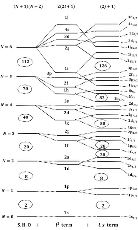
where N is the oscillator quantum number, n is the radial quantum number, and l is the orbital angular momentum quantum number. The value of N in each oscillator shell degenerates to a set of levels, with either even or odd values of the allowed orbital angular momentum (l=N, N-2,...,1 or 0). The equally-spaced levels (major shells) could be occupied by maximum number (N+1)(N+2)of identical nucleons. The parity of each level is given by:
π = (−1)l = (−1)N (2.5)
The labelling of the levels and the occupation limit of the shells of harmonic oscillator potential are illustrated in table 2.1.
N Allowed l Level Label (n,l) EN(¯hω0) Occupation P2(2l+ 1) Total
0 0 1s 3/2 2 2
1 1 1p 5/2 6 8
2 2, 0 1d, 2s 7/2 12 20
3 3, 1 1f, 2p 9/2 20 40
4 4, 2, 0 1g, 2d, 3s 11/2 30 70
5 5, 3, 1 1h, 2f, 3p 13/2 42 112
6 6, 4, 2, 0 1i, 2g, 3d, 4s 15/2 56 168
Table 2.1: Occupation of harmonic oscillator shells.
a more realistic form with contributions of an attractive term l2 and a spin-orbit
interaction. The l2 term refines the shape of the potential to an intermediate shape
between the square well and harmonic oscillator potentials and lowers the energy levels of the higher orbital angular momentum states, as illustrated in the middle part of Figure 2.1. The latter term will be disused in the next section.
2.3.2
Spin Orbit Interaction
The effect of the total angular momentum of each single nucleon in the nucleus has been taken into account (increased) using the harmonic oscillator potential by Mayer and Haxel [May49], Jensen and Suess [Hax49], in the form of a spin-orbit interaction,
VSO =−f(r)l.s (2.6)
where,landsare the orbital angular momentum and intrinsic spin quantum numbers for the single nucleons respectively, and f(r), is the strength of interaction, which is given by
f(r) =λ1 r
dV(r)
dr (2.7)
�.�.� + � � + �.� �
Type equation here.
�=
/
/ / /
�/
/
�/
/
�/
�/
�=
�=
�
�=
/
/
�+ �+ �+ ( �+ )
�
�/
/
/ /
�/
/ /
/
/
/ 2f7/2
1h9/2
�=
�=
�=
/ / /
/
/
[image:33.595.143.422.117.581.2]�
Figure 2.2: Single particle energy levels of the harmonic oscillator potential with the effects of l2 term and spin-orbit interaction.
2.3.3
Woods-Saxon Potential
The Woods-Saxon (WS) potential is considered to be the most realistic form of the nuclear potential compared with the infinite square well and harmonic oscillator po-tentials. The shape of this finite potential is most likely as it follows distribution of the nuclear matter, smoothly vanishes outside the nucleus. It has the form [Woo54],
VW S(r) = −
V0
1 +exp[r−aR0]
(2.8)
where V0 is the depth of the potential. R0 and a are the radius and the surface
dif-fuseness of the nucleus respectively. The Woods-Saxon potential will produce energy levels the same as of the harmonic oscillator potential with thel2 term, and reproduce
the correct magic numbers with the addition of a spin-orbit interaction.
2.4
Nuclear Deformation
The spherical shell model has been successful in predicting the single particle prop-erties for nuclei near closed shells. Despite these successes, discrepancies have been observed between the theoretical predictions and experimental results with increas-ing numbers of nucleons outside closed shells. For instance, the nuclear quadrupole moment in the ground state has been found to change with nucleon number between major shells and is very large for certain nuclei. This behaviour is clear evidence for existence of static deformation in nuclei with atomic masses A∼= 25, 150< A <190 and A > 220. Thus the nuclear potential deviates from its spherical symmetry to a deformed shape. The shape of a deformed nucleus can be parameterised through the expansion of the nuclear radiusR(θ, φ) in polar coordinates in terms of spherical harmonics Yλ,µ(θ, φ),
R(θ, φ) =Ro
1 +
∞ X
λ=0
λ
X
µ=−λ
αλµYλµ(θ, φ)
(2.9)
Where Ro is the radius of the sphere of the same volume of the deformed nucleus
nuclear surface with respect to the equilibrium shape. Coefficients of λ=0 and λ=1 corresponds to the conservation and translation of the nuclear volume respectively, were assumed to be equal to zero. The most significant deformations occur in nuclear shape with λ=2, quadruple deformation, which describes the elongation of axially symmetric shape of the nucleus. The five coefficients of α2µ can be written in,
α20 =β2cosγ, α21 =α2−1 = 0, α22 =α2−2 =
1
√
2β2sinγ (2.10) where β2 represents quadrupole deformation parameter of the nucleus and γ
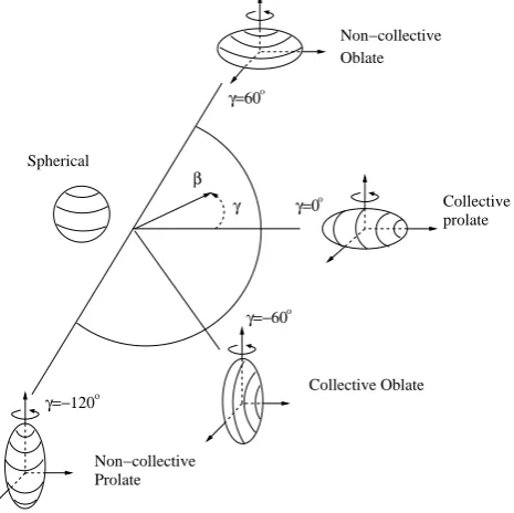
indi-cates the triaxiality of the nucleus and corresponds to the deviation from the axial symmetry. The various shapes of the nucleus in the (β2, γ) coordinates can be
repre-sented by Lund conversion [And76], as in Figure 2.3. For quadrupole deformations, the axially symmetric collective shapes are prolate at γ = 0◦ or oblate at γ = −60◦, while the non collective shapes can be seen at γ = −120◦ and 60◦ respectively. The triaxial shapes of the deformed nucleus along z-axis can be observed in the sector of the (β2, γ) plane, when triaxial parameter changes between angles 0◦ < γ <60◦.
Spherical
Oblate Non−collective
Collective prolate
Collective Oblate
Non−collective Prolate
β γ γ=60
γ=0
γ=−60
γ=−120ο
[image:35.595.266.499.437.669.2]o o o
2.5
The Anisotropic Harmonic Oscillator
Poten-tial
The deformed potential is used to describe nuclei with shapes deviated from sphericity. The potential for axially symmetric nuclei along z-axis (x=y6=z) is represented by anisotropic harmonic oscillator [Nil69],
VAHO =
1 2M
ω⊥2(x2 +y2) +ω2zz2
(2.11)
where ω⊥ and ωz are the oscillator frequencies in the directions parallel and
per-pendicular to the symmetry axis respectively. They can be related to the oscillator frequency in the spherical case ω0 and to the deformation parameterε,
ωz ≈ω0
1− 2
3ε
, ω⊥ ≈ω0
1 + 1
3ε
(2.12)
Thus, the oscillator frequencies ensure the volume conservation ω3
0 =ω2⊥ωz. The
os-cillator frequencyω0 can be deduced from the energy difference between two adjacent
major shells and the expectation value of the nuclear radii for protons and neutrons [Won98],
¯
hω0 = 41A−1/3
1± N −Z
3A
M eV (2.13)
The numerical values for nuclear wave functions show thatω0has isospin dependence,
so the positive sign used for neutrons and negative sign for protons. Nilsson [Nil55] transformed the problem of the anisotropic harmonic oscillator potential to stretched coordinates (ξ, η, ζ), in order to introduce the deformed potential in terms of the deformation ελ parameters and the angle of the stretched coordinates. The potential
for the λ= 2 case is given by [Nil69],
VAHO =
1
2¯hω0(ε2)ρ
21−2
3ε2P2(cos(θt)
(2.14)
The parameterρis defined as the radius in the stretched coordinates,ρ2 =ξ2+η2+ζ2,
θt = cos−1(ζρ), and ε2 is the quadrupole deformation in the stretched coordinates,
the ε4ρ2P4(cosθt) term is added to the potential. The eigenvalues of the Hamiltonian
for the anisotropic harmonic oscillator potential are given by:
EN nzn⊥ ≈
N +3 2
¯ hω0−
1
3ε(2nz −n⊥)¯hω0 (2.15) and
N =nz+n⊥ (2.16)
Where N is the major oscillator quantum, nz is the number of oscillation quanta
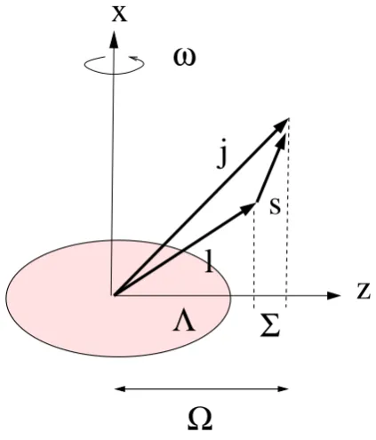
in the wave function along the symmetry axis. The single particle eigenstates in the deformed nuclear potential are labelled with asymptotic quantum numbers [N nzΛ]Ωπ,
Λ and Ω are the projections of the orbital and total angular momentum onto the symmetry axis respectively, and π is the parity of states identified by −1N. The
projection of total angular momentum on the symmetry axis is defined Ω = Λ±Σ = Λ± 1
2, where Σ is the projection of the intrinsic spin of the single particle onto the
symmetry axis. Figure 2.4 illustrates this for a deformed axially symmetric nucleus in the absence of rotation.
x
z
ω
Ω
j
Σ
Λ
s
[image:37.595.232.444.439.687.2]l
2.6
Nilsson Model
Nilsson introduced a unified nuclear model to describe the structure of the nucleus in a deformed potential and explain the behaviour of the single particle states with deformation. The potential that has been used in the Nilsson model is based on the anisotropic harmonic oscillator potential with contribution of a spin-orbit interaction and a l2 term, which is known as Modified Harmonic Oscillator (MHO) potential or
Nilsson Potential. Its most common form is written as;
VM HO =VAHO −κhω¯
2l.s+µ(l2− hl2iN)
(2.17)
where κ and µ are adjustable coupling parameters, which are estimated for each major shell differently by fitting with the observed energy levels of the deformed nuclei experimentally. The κ¯hω[2l.s+µ(l2− hl2i
N) term is added to reproduce the
correct magic numbers and restore the spacing between two adjacent major shells as in the case of the spherical nucleus. Furthermore, the Nilsson potential splits each j shells in the spherical shell model at zero deformation into j + 1/2 and j −1/2 states. Each state is specified by the projection of total angular momentum on the symmetry axis Ω and its parity π , which are the only conserved quantum numbers, and the states are twofold degenerate according to ±Ω. In the Nilsson model, the eigenvalues of Hamiltonian are represented as the diagrams of single particle energies of the nucleons as a function of quadrupole deformation, known as Nilsson diagrams. Figures 2.5 and 2.6 show Nilsson diagrams for neutrons and protons respectively. The energy of the eigenstates changes according to the spatial orientation of the orbits with respect to the nuclear symmetry axis. The levels of lowest Ω value are from the highest possible nodes of the wave function in the direction of the symmetry axis and their energies decrease with increasing prolate deformation, while the levels of higher Ω value are higher in energy and have a lower nz value, (N =nz+ Λ, where Λ can be
−0.3 −0.2 −0.1 0.0 0.1 0.2 0.3 0.4 0.5 0.6 5.0 5.5 6.0 ε2 E s.p. (h −ω ) 50 82 1g9/2 2d5/2 1g 7/2 3s1/2 1h11/2 2d3/2
3/2[301] 3/2
[541] 5/2[303] 1/2 [301] 1/2[301] 1/2 [550] 1/2 [440] 3/2 [431] 3/2 [431] 5/2 [422] 5/2 [422] 7/2[413] 7/2[413] 9/2[404] 9/2 [404] 1/2 [431] 1/2 [431] 3/2[422] 3/2 [422] 5/2[413] 5/2 [413] 1/2 [420] 1/2 [420] 1/2 [660]
3/2 [411] 3/2
[651]
5/2 [402] 5/2
[image:39.595.129.511.133.632.2][402] 5/2 [642] 7/2[404] 7/2[404] 1/2 [411] 1/2 [411] 1/2 [660] 1/2 [420] 1/2[550] 1/2 [550] 1/2 [541] 3/2 [541] 3/2 [541] 3/2 [301] 5/2 [532] 5/2 [532] 7/2[523] 7/2 [523] 9/2[514] 9/2[514] 11/2 [505] 11/2 [505] 1/2 [400] 1/2[400] 1/2 [660] 1/2 [411] 1/2 [651] 3/2[402] 3/2 [411] 1/2 [541] 1/2 [301] 3/2 [532] 7/2 [514] 1/2 [530] 1/2 [770] 3/2 [521] 3/2 [761] 9/2 [505] 1/2 [660] 1/2[400] 1/2 [411] 3/2 [651] 3/2[402] 5/2 [642] 5/2 [402] 13/2 [606] 1/2 [770] 1/2 [530] 3/2 [521] 1/2 [761] 1/2 [400] 1/2 [640] 1/2 [880] 1/2 [640]
Figure 2.5: Nilsson diagram of single-neutron energies (50< N < 82) as a function of the quadrupole deformation parameter ε2. Full and dashed lines correspond to
−0.3 −0.2 −0.1 0.0 0.1 0.2 0.3 0.4 0.5 0.6 5.0 5.5 6.0 ε2 E s.p. (h −ω ) 50 82 1g9/2 1g7/2 2d5/2 1h11/2 2d3/2 3s1/2
3/2[301] 3/2 [541] 5/2[303] 1/2 [301] 1/2[301] 1/2 [550] 1/2[440] 3/2 [431] 3/2 [431] 5/2 [422] 5/2 [422] 7/2[413] 7/2[413] 9/2 [404] 1/2 [431] 1/2 [431]
3/2[422] 3/2[422]
5/2[413] 5/2 [413] 7/2[404] 7/2[404] 1/2 [420] 1/2 [420] 1/2 [660] 3/2[411] 3/2 [411] 3/2 [651] 5/2 [402] 5/2[402] 5/2 [642] 1/2[550] 1/2 [550] 1/2[301] 1/2 [541] 3/2 [541] 3/2 [541] 3/2[301] 5/2 [532] 5/2 [532]
7/2 [523] 7/2 [523]
9/2[514] 9/2[514] 11/2 [505] 11/2 [505] 1/2 [411] 1/2 [411] 1/2 [660] 1/2 [420] 3/2 [402] 3/2 [651] 3/2 [411] 1/2[400] 1/2 [660] 1/2 [651] 1/2 [541] 1/2 [301] 3/2 [532] 5/2 [523] 7/2[514] 9/2 [505] 1/2 [660] 1/2 [400] 1/2 [651] 1/2 [411] 3/2 [651] 3/2 [402] 3/2 [642] 5/2 [642] 5/2 [402] 7/2 [633] 11/2 [615] 13/2 [606] 1/2 [530] 3/2 [521] 3/2 [761] 1/2 [770] 3/2 [521] 1/2 [761] 1/2 [640]
Figure 2.6: Nilsson diagram of single-proton energies (50 < N < 82) as a function of the quadrupole deformation parameter ε2. Full and dashed lines correspond to
shell are different in energy because of the isospin dependency of anisotropic harmonic oscillator. However at certain deformations low density regions of single particle states arises (deformed magic numbers) in the Nilsson spectra as a consequence of repulsive interaction between states of the same Ωπ. These states approach each other and
interchange the properties of their wave functions according to the Pauli Exclusion Principle.
2.7
The Strutinsky Shell Correction Procedure
In the previous sections, the nucleus has been described using two different concepts. The liquid drop model takes into account the contribution of all nucleons in the nucleus to calculate the nuclear binding energy and the macroscopic properties of the nucleus. In contrast, the shell model assumes that the protons and neutrons move in individual orbitals independently from one another in a certain average nuclear potential from all other nucleons in the nucleus. Particular nuclear properties can be identified from the behaviour of the specific single particles near to the Fermi surface. It is clear that both models ignore the influence of each other in the calculation of the total energy of the nucleus. This discrepancy led Strutinsky to propose the shell correction procedure [Str67, Str68] to obtain accurately the total energy of the nucleus and the nuclear ground state energies as a function of deformation. The shell correction procedure combines the successful features of the two models, in which, Strutinsky added an oscillatory energy from the microscopic shell model to the predicted nuclear binding energy from the liquid drop model.
E =ELDM + ∆Eshell (2.18)
This oscillatory energy (∆Eshell) arises from the fact that the nuclear binding energy
This correction in the model enabled the nuclear ground state energies as a function of deformation to be determined accurately, which are generally presented in the form of the potential energy surfaces of the nucleus.
2.8
Pairing and Quasiparticles
The pairing correlation is the characteristic of the strong nuclear force in the form of a short-range component between any two nucleons, which originates from the spatial overlap of the identical particles with the same quantum numbers and opposite spins, consequently their angular momenta couple to I = 0. The inclusion of the pairing interaction to the nuclear structure model was the key answer for a number of out-standing experimental observations, which could not be interpreted in the framework of the single particle shell models. For instance;
• The spin and parity (Iπ) of the ground state in all even-even nuclei is 0+.
• The energy difference between the first non-collective excited state and the ground state in even-even and even-odd nuclei.
• The differences in masses and binding energies of even-even and even-odd nuclei are related to the odd-even effect, the role of the last nucleon in the pairing regime. The masses of odd-even nuclei are higher than the average mass of the two neighbouring even-even nuclei, while in even-even nuclei all nucleons are paired and have higher binding energies.
• Nuclei in the region near the closed shells or close to closed shells preserve a spherical shape, because the influence of the pairing force overcomes the ten-dency to deform.
( ) ( )
∆ ∆
� �
without pairing with pairing
�
�
�
���
�
Figure 2.7: The left figure illustrates a pair of nucleons in time reversed orbital (a), scattered into another time reversed orbital (b). The figure on the right side illustrates the single particle occupation probability as a function of single particle energy and explains the effect of pairing correltion on the Fermi surface.
The Pauli Exclusion Principle does not allow paired particles to orbit in the same level, so each nucleon in a pair orbits in the time reversed orbits and to complete one orbit they scatter twice into free orbits of a different energy state near to the Fermi surface, as illustrated in Figure 2.7. Thus the scattered pairs in the time reversed orbits smear the Fermi surface in the energy domain over an energy of twice the pairing gap (∆), and this simultaneous interaction process will produce a mixture of occupied (particle) and unoccupied (hole) states below and above Fermi surface. This scattering model is considered as the fundamental concept to introduce quasi-particles, which represent the partially occupied (particle-hole) states with unity oc-cupation probability in terms of the probability of fullnessV2
i and emptinessUi2 of the
orbits. Therefore the particle-hole excitation is replaced by the simultaneous creation and annihilation operator of quasiparticles. The quasiparticle energy of a state i in the presence of paring interaction is given by;
Ei =
q
where, i is the single-particle energy, λ is the Fermi energy and ∆ is pair gap which
Nuclear Rotation
3.1
Introduction
Rotation of spherically symmetric nuclei in space is forbidden in quantum mechanics, as those nuclei are invariant under rotation. When the shape of nucleus deviates from spherical symmetry, as shown in Figure 3.1, it possesses a deformed shape and rotates around one of the axes (x or y) perpendicular to the symmetry axis (z). Hence, the angular momentum of the rotated nuclear system is generated in two different mechanisms, non-collective excitation of unpaired valence nucleons and collective excitation of the rotating core (paired nucleons). Therefore, this chapter will introduce some basic concepts of nuclear rotation and discuss the interplay between collective and single particle modes to describe nuclear structure phenomena observed from the experimental spectra of the rotating nucleus.
3.2
Non-Collective Single Particle Excitation
In the region close to the closed shells, nuclei have spherical or near spherical shapes. Nuclear angular momentum in these nuclei is only generated non-collectively, by the alignment of the individual spins of the valance nucleons along the rotation axis which coincides with to the symmetry axis, as shown in Figure 3.2a. This mechanism gives
�
� � �
�
�
Figure 3.1: Illustrates rotation of an axial symmetric nucleus around an axis per-pendicular to the symmetry axis, and its angular momenta projections.
rise to a large value of total angular momentum (J) of the nucleus corresponding to the sum of the single particle contributions of high j and large Ω orbitals near to the Fermi surface. Nuclear excited states that are based on this mode of angular momentum generation are known as single particle excited states which can be observed in both spherical and deformed nuclei.
3.3
Collective Excitation
The deformed nucleus rotates collectively around an axis perpendicular to the symme-try axis. All nucleons in the rotating core contribute to generate angular momentum coherently, which increases with rotational velocity of the nucleus. The total angular momentum of the nucleus, is identified from the vector coupling of angular momenta which is generated by the single particle contributions of the valance nucleons J, and of the rotated core R, as illustrated in Figure 3.1.
I=R+J (3.1)
The projection of total angular momentum onto the rotation axis Ix is defined as;
Ix =
q
Figure 3.2: (a) Generation of angular momentum and single particle excite states in a near spherical nucleus 147Gd as a consequence of single particle excitation. (b)
Collective rotation in a deformed nucleus to generate angular momentum collectively and exhibit a rotational band in 158Er.
Where, K is the projection of total angular momentum onto the symmetry axis. The collective rotation of an axially symmetric deformed nucleus exhibit different se-quences of rotational spectra between successive sets of intrinsic nuclear excited states, known as rotational bands of different static moment of inertia J, their energies are given by:
E(I, K) = ¯h
2
2J [I(I + 1)−K
2] (3.3)
Single nucleons can not build angular momentum in even-even deformed nuclei up to spin 10-12¯h, because all nucleons are paired in the ground state. For K=0 band, rotational energy in the above relation can be expressed as:
E(I) = h¯
2
2JI(I+ 1) (3.4)
of gamma-ray with energy,
Eγ =E(I)−E(I−2) =
¯ h2
2J(4I−2) (3.5)
3.4
Rotational Frequency and Moment of Inertia
In the experimental investigation of high spin states, the behaviour of a rotating deformed nucleus is usually described in terms of rotational frequency. The rotational frequency is related to the energy difference between successive states of a rotational band, and approximately equal to half the energy of the emitted gamma-ray [Ray73];
¯
hω = dE dIx
= ∆(EI−EI−2)
∆I =
Eγ
2 (3.6)
This quantity varies with angular velocity, as a consequence of the changes that occur in the structure of a deformed nucleus during rotation. So, to explain the behaviour of rotating deformed nucleus, Bohr and Mottelson [Boh81] introduced kinematicJ(1)
and dynamic J(2) moments of inertia. The kinematic moment of inertia describes
the rotating system of the deformed nucleus and is defined as:
J(1) =
2
¯ h2
dE(I) dIx
−1
= ¯hI
ω (3.7)
The dynamic moment of inertia J(2) explains the influence of competition between
interactions that are taking place in the structure of rotational bands in a deformed nucleus during rotation, and is defined as:
J(2)= 1
¯ h2
d2E(I)
dI2
x
−1
= ¯hdI
dω (3.8)
J(1), can be related to energy of the gamma-ray emitted in the rotational band for a
given spin value,
J(1) = ¯h2(2I−1) Eγ
(3.9)
In addition,J(2) can be calculated from the energy difference between of consecutive
gamma-ray,
J(2) = 4¯h 2
∆Eγ
Therefore, it is clear that J(2) does not depend on the spins of the excited states of
the rotational band.
3.5
Particle-Rotor Coupling
The particle-rotor model [Ste72] is based on the prediction of Mottelson and Valatin [Mot60] for the Coriolis force. When the deformed nucleus rotates around the axis perpendicular to the symmetry axis, this Coriolis force tries to decouple the valance nucleons that are bound to the rotating deformed core of the nucleus. The maximum Coriolis force exerted on a particular valence nucleon with angular momentum j, in the potential of a deformed rotating nucleus of total angular momentum I can be defined as [Ste75],
EmaxCor ≈(h¯
2
J )J.I (3.11)
The above relation illustrates that the nucleons in high j orbitals (intruder orbitals) are very sensitive to this force. In the particle rotor model, the motion of nucleonic system (a valence nucleon and a core of the paired nucleons) is only constrained by the strength of the potential of the deformed core and the Coriolis force which is induced by the rotation of the nucleus. There are two different coupling limits: the deformation aligned limit (DAL) and the rotational alignment limit (RAL). Figure 3.3 illustrates the two coupling limits.
� �
�
�
��
�=�
� �
��
� �
�=�
( ) ( )
Figure 3.3: Particle rotor coupling scheme (a) Deformation aligned and (b) Rota-tional alignment.
3.6
The Cranking Model
The Cranking model was introduced by Inglis [Ing54, Ing56], to explain the micro-scopic description of behaviour of the rotating nucleus around an axis of rotation, perpendicular to the symmetry axis, under influence of a deformed nuclear potential field along the symmetry axis. In the Cranking model single-particle and collective excitations of the nucleus are taken into account as independent particles moving in a rotating potential with constant angular velocityω. The energy of independent single particles in the rotating system has been identified by using a cranking Hamiltonian (Routhian). The transformation of the intrinsic coordinate system to the rotating frame reference is through the rotation operator.
ˆ
Rx = exp−iωtix (3.12)
The cranking Hamiltonian for an independent single particle takes the following form:
hω =hint−¯hωix (3.13)
The cranking Hamiltonian over all the independent single particles of the system defines the total cranking Hamiltonian of the rotating nucleus as,
Hω =Xhω =Hint−¯hωIx (3.14)
Where, Hint is sum of the single particle Hamiltonians in the intrinsic frame of
ref-erence, and Ix represents the sum of the projections of all single particle angular
momenta onto the rotation axis. The term ¯hωIx in the above equation represents
Coriolis and centrifugal forces in the rotating coordinate system. The effect of this term has been taken into account for single particle energies of the deformed shell model (Nilsson model) by Bengtsson and Frauendorf [Ben79], and introduced in the form of the Cranked Shell Model (CSM). The various forms of CSM [Naz85, Cwi87] can be used to interpret the structure of nuclei at high angular momentum, in terms of quasiparticle configurations and either quasiparticle or single particle Routhains for protons and neutrons independently, as in the case of159Er that will be presented
3.7
Nuclear Symmetries
In the introduction of rotation to an axially symmetric nucleus, the two fold degen-eracy of Nilsson orbits with respect to time reversal symmetry (±Ω) is broken by the Coriolis force and results in Nilsson orbits split into two single particle levels. The splitting between the two levels depends on the projection of the single particle angu-lar momentum onto the rotation axis corresponding to that orbit, and increases with rotational frequency. Consequently, the only remaining symmetries for the cranking Hamiltonian are invariance with respect to the spatial reflection and with rotations of 180◦ around the axis of rotation. These two symmetries are called parity (π) and signature (α). They label the nuclear states of the rotating nucleus, and will be outlined in next two sections. A schematic illustration of the effect of cranking on the single particle energy levels of Nilsson orbits originating from principal quantum number N=2, in a harmonic oscillator potential is illustrated in Figure 3.4.
�
�=
�
�
�/
� /
��/
��
���������: �+ �+ �+ �+ ������� ������: �,� �,�,� �,�,�,� ���� �� �,�
�
(+,−)
(�,�)
(+, +)
(+,−)
(+, +) �������� ����� ����� ������� �������+
��������� ����� ���� ������� ���������
�.� ℏ���
/ +
/ +
�/ +
/ +
/ +
ℏ� �
3.7.1
Parity
Parity is an operator which describes the reflection symmetry through the origin of the spatial part of particle wavefunction relative to all coordinates. The eigenvalues of the parity operator ˆπψ(−~r) have two values, firstly;
ψ(−~r) = +ψ(~r) (3.15)
The reflected wavefunction remains unchanged and the parity will be even, then the parity of single particle state is labelled +, and if;
ψ(−~r) = −ψ(~r) (3.16)
this means that the reflected wavefunction is inverted and parity is odd. Here the parity of single particle state is labelled−. The total parity of a nuclear state is given by the product of the parities of all occupied single particle orbitals:
πtotal =
Y
occ
πi, (3.17)
3.7.2
Signature
Signature arises from the invariance of the cranking Hamiltonian with respect to a rotation of 180◦ around the x-axis through the rotation operator ˆR [Syz83],
ˆ
Rx = exp−iπIx (3.18)
The eigenvalues (r) of the rotation operator, result in the signature exponent quantum number (α),
r≡exp−iπα (3.19)
The allowed values of eigenvalues are restricted to the total number of nucleons in the rotating nucleus that are of even or odd A.
For even-A nucleus, r takes values +1 and −1 with α = 0 and 1 respectively, giving rise to nuclear states of spin
I = 1,3,5,7, ... (3.21) Whereas for odd-A nucleus,rhas values−iand +iwithα= +12 and−12 respectively,
I = 1 2,
5 2,
9 2,
13
2 , ... (3.22)
I = 3 2,
7 2,
11 2 ,
15
2 , ... (3.23)
Experimental Details
4.1
Introduction
The following chapter will describe the reaction carried out to populate the excited states in 159Er up to ultra high spin. The interactions in the detection system used
during the experiment will also be discussed. In addition, the spectroscopic techniques that were employed in the work to identify and study the nuclear structure of the populated nucleus will be outlined.
4.2
Heavy Ion Fusion Evaporation Reaction
The Heavy Ion Fusion Evaporation Reaction has been employed to populate the highest spin states in nuclei [New70]. Niels Bohr in 1936 proposed using the fusion mechanism of projectile on target in nuclear reactions to form a compound nucleus [Boh36]. In fusion, the projectile beam of heavy ions may fuse with the target nucleus to form a highly excited compound nucleus at high spin, provided that the centre of mass energy is sufficient to overcome the Coulomb barrier between projectile and target nuclei [Hod78]:
ECB =
ZpZte2
RCB
M eV (4.1)


![Table 5.3: The measured properties of the transitions in Band 2 of 159Er, *[Str75].](https://thumb-us.123doks.com/thumbv2/123dok_us/8072819.227209/86.595.111.564.126.798/table-measured-properties-transitions-band-er-str.webp)


