This is a repository copy of
Structure of the species-energy relationship
.
White Rose Research Online URL for this paper:
http://eprints.whiterose.ac.uk/1419/
Article:
Bonn, A., Storch, D. and Gaston, K.J. (2004) Structure of the species-energy relationship.
Proceedings of the Royal Society B: Biological Sciences, 271 (1549). pp. 1685-1691. ISSN
1471-2954
https://doi.org/10.1098/rspb.2004.2745
eprints@whiterose.ac.uk https://eprints.whiterose.ac.uk/ Reuse
Unless indicated otherwise, fulltext items are protected by copyright with all rights reserved. The copyright exception in section 29 of the Copyright, Designs and Patents Act 1988 allows the making of a single copy solely for the purpose of non-commercial research or private study within the limits of fair dealing. The publisher or other rights-holder may allow further reproduction and re-use of this version - refer to the White Rose Research Online record for this item. Where records identify the publisher as the copyright holder, users can verify any specific terms of use on the publisher’s website.
Takedown
If you consider content in White Rose Research Online to be in breach of UK law, please notify us by
Published online6 July 2004
Structure of the species–energy relationship
Aletta Bonn
1*, David Storch
2,3and Kevin J. Gaston
11Biodiversity and Macroecology Group, Department of Animal and Plant Sciences, University of Sheffield,
Sheffield S10 2TN, UK
2Center for Theoretical Study, Charles University, Jilska´ 1, 110 00-CZ Praha 1, Czech Republic
3Santa Fe Institute, 1399 Hyde Park Road, Santa Fe, NM 87501, USA
The relationship between energy availability and species richness (the species–energy relationship) is one of the best documented macroecological phenomena. However, the structure of species distribution along the gradient, the proximate driver of the relationship, is poorly known. Here, using data on the distribution of birds in southern Africa, for which species richness increases linearly with energy availability, we provide an explicit determination of this structure. We show that most species exhibit increasing occupancy towards more productive regions (occurring in more grid cells within a productivity class). However, average reporting rates per species within occupied grid cells, a correlate of local density, do not show a similar increase. The mean range of used energy levels and the mean geographical range size of species in southern Africa decreases along the energy gradient, as most species are present at high productivity levels but only some can extend their ranges towards lower levels. Species turnover among grid cells consequently decreases towards high energy levels. In summary, these patterns support the hypothesis that higher productivity leads to more species by increasing the probability of occurrence of resources that enable the persistence of viable populations, without necessarily affecting local population densities.
Keywords:species–energy relationship; species–area effect; productivity; occupancy; species turnover
1. INTRODUCTION
The covariation between the number of species in an area and the availability of environmental energy is fundamen-tal to an understanding of spatial variation in species rich-ness (Wright 1983; Turner et al. 1988; Currie 1991; Gaston 2000; Kaspari et al. 2000; Hurlbert & Haskell 2003). Studies so far have primarily concerned the estab-lishment of the form and occurrence of species–energy relationships. These have variously been found to be posi-tive, negative and hump-shaped. Some examples of the first two comprise the extremes of the third, but others apparently do not, and there is growing evidence for dependence of the form of observed patterns on spatial scale (Waideet al. 1999; Mittelbachet al. 2001; Whittaker et al. 2001; Chase & Leibold 2002; Van Rensburget al. 2002). Such complexity has, perhaps inevitably, led to a multitude of explanations for species–energy relationships, rooted in a variety of evolutionary and ecological processes (Kerr & Packer 1997; Rohde 1997; Rosenzweig & Sandlin 1997; Srivastava & Lawton 1998; Allen et al. 2002; Storch 2003).
As with other macroecological patterns, untangling the causes of the species–energy relationship is problematic, because the large-scale nature of the pattern does not allow direct experimental testing (although manipulations of ‘model’ systems at smaller scales may prove informative (Gaston & Blackburn 1999)). However, although it is dif-ficult to definitively prove or reject the importance of any particular process potentially leading to the relationship, it is possible to strengthen the support for some hypo-theses and weaken that for others, by detailed analysis of
*Author for correspondence (a.bonn@sheffield.ac.uk).
Proc. R. Soc. Lond.B (2004)271, 1685–1691 1685 2004 The Royal Society
the structure of the pattern; i.e. of the distribution of indi-vidual species along the energy gradient. In practice, although some other predictions of mechanisms proposed to determine species–energy relationships have been tested (e.g. Srivastava & Lawton 1998; Gaston 2000; Kaspariet al. 2003), this approach has not, to our knowledge, been used.
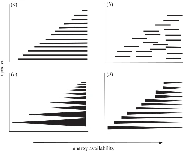
Assuming a linearly increasing species–energy relation-ship, we can distinguish two extreme types of species dis-tribution along the energy gradient. First, species may exhibit a nested occurrence pattern, such that those present at a given level of energy availability always occur at higher ones (figure 1a; note that this pattern leads to a decrease in the average range of species occurrence along the gradient). Second, species can occupy equally narrow ranges along the gradient, regardless of the energy level (figure 1b). Real patterns of species distribution will prob-ably lie somewhere between these two extremes. However, patterns closer to the ‘nested’ one indicate that greater energy availability increases the chance of persistence of most species independently to each other, i.e. in an indi-vidualistic manner. On the contrary, the other extreme type of distribution supports the role of processes affecting whole species assemblages, either as a result of the evol-ution of separate species pools in areas with different energy levels (e.g. faster evolution in areas with higher lev-els of energy (see Rohde 1997; Allen et al.2002)), or as a result of the sorting of species along the gradient by interspecific competition (Rosenzweig & Abramsky 1993; Rosenzweig 1995) or other evolutionary processes.
1686 A. Bonn and others Structure of species–energy relationship
(a) (b)
(c) (d)
species
[image:3.598.150.445.60.303.2]energy availability
Figure 1. Extreme patterns in species distribution along an energy gradient leading to higher richness at higher energy levels. (a) The nested distribution: all species can occur in higher energy levels, but not all can thrive in low levels of available energy. (b) Species range sizes are not related to energy level, but more species are confined to higher energy levels. (c) Species abundances increase with increasing energy, enabling the persistence of less common species. (d) Species abundances decrease with increasing energy, as a consequence of increasing interspecific competition or environmental heterogeneity.
relationship between energy availability, the overall amount of resources in an area, the total number of indi-viduals that can thus be maintained, and consequently the number of species. This predicts that individual species will probably be more abundant with increasing energy availability (figure 1c), that they will occupy more sites with increasing energy availability, and also that at lower energy levels there will be higher turnover in species ident-ities among sites than at higher ones (at which most spe-cies can maintain viable populations in most places). By contrast, what we shall call the ‘specialization’ hypothesis assumes that higher energy levels enable finer sub-division of available resources, either because of reductions in niche breadth or through the generation of greater resource diversity or habitat heterogeneity (e.g. Abrams 1995; Kerret al.2001). This predicts that individual spe-cies may become less abundant with increasing energy availability (figure 1d), that they will occupy fewer sites at higher energy availability, and also that there will tend to be higher turnover of species among sites at higher levels of energy availability than among sites at lower availability (see Whittaker 1960; Gaston & Williams 1996; Brown & Lomolino 1998).
In this paper, we determine the key features of the struc-ture of a species–energy relationship, focusing on the dis-tribution of individual species along the energy gradient. We use as a case study the avian species assemblage of South Africa and Lesotho, for which the existence of such a relationship is already well established (Van Rensburget al.2002). First, we describe (i) the observed pattern and test whether the observed species–energy relationship is attributable to (ii) the species–area relationship, as the existence of such an effect could influence subsequent considerations (Rosenzweig 1995). Then we analyse (iii) the relationship between energy and species’ environmental
Proc. R. Soc. Lond.B (2004)
and geographical ranges. We subsequently test whether higher energy levels lead to higher levels of (iv) occupancy and (v) abundance of species. Finally, we analyse (vi) trends in species turnover along the energy gradient.
2. METHODS
(a) Data
Avian species-richness data for South Africa and Lesotho were obtained from the Southern African Bird Atlas Project (Harrison et al. 1997), which compiled information, mainly collected between 1987 and 1992, on species occurrences on a quarter-degree grid (15⬘×15⬘⬇676 km2). We consider presence or absence and reporting rate data for 651 native species excluding marine, vagrant, marginal and introduced or escaped species. Reporting rates are the proportion of checklists submitted for each grid cell with presence records for a given species, and reflect broad differences in local abundances (Robertsonet al. 1995).
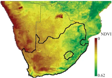
We used the normalized difference vegetation index (NDVI) as a measure of energy availability. A mean 9 year average NDVI for the first decade in January (1982–1991) for each quarter-degree grid cell was obtained from the African Real Time Environmental Monitoring using Meteorological Satellites pro-gram (Artemis) of the Food and Agriculture Organization (FAO; see http://metart.fao.org/default.htm). In January, differ-ences in the NDVI index were most pronounced and ranged from 0 to 0.63 across the whole of Africa at a 0.01 resolution. The means for quarter-degree grid cells across the region of interest span 0.04 to 0.50 (at the original spatial resolution of 7.6 km2the values span 0.0 to 0.54). Substantially higher levels than these are only met by moving considerable distances beyond the borders of South Africa (figure 2).
NDVI 0
[image:4.598.54.291.60.224.2]0.62
Figure 2. A map of the southern part of the African continent showing NDVI levels. The study area, South Africa and Lesotho, is delineated with bold black boundaries. NDVI classes are relatively contiguous in the study area, and the areas of intermediate productivity exhibit the greatest surface area and areal coverage.
measures of net primary productivity (NPP) (Woodwardet al. 2001) that have previously been employed in documenting a species–energy relationship for the South African avifauna (Van Rensburget al.2002). However, at a half-degree resolution the two are closely correlated (r2=0.81,p⬍0.001). Moreover, the following analyses, when performed using NPP as the energy variable at the broader resolution, arrived at similar results.
(b) Analyses
We recognize two scales of analysis. The first is that of the quarter-degree grid cell, and the number of species occurring in a cell is termed grid-cell species richness. The second is that of the NDVI class, and the total number of species occurring in one or more grid cells within a class is termed NDVI class species richness. The grid cells fall into 47 classes from lowest to highest NDVI values, with 0.01 increments of NDVI (finest possible resolution).
To determine relationships between species richness and NDVI, linear and quadratic regressions were performed. When quadratic effects were found significant, we used a statistical test developed by Mitchell-Olds & Shaw (1987) (see also Chase & Leibold 2002) to test for the significance of a hump-shaped relationship, determining whether the estimated maximum of species richness in intermediate levels of NDVI is significantly greater than species richness at both low and high NDVI levels. As spatial autocorrelation may systematically distort classical tests of association, we implemented spatial correlation models for analyses at the grid-cell level using the Proc Mixed pro-cedure (Littellet al.1996). An exponential covariance structure was used as it gave a better fit to the null model, as assessed by Akaike’s Information Criteria and Schwarz’s Bayesian Criteria. To test for potential species–area effects on the species–energy relationship, the number of cells falling within each NDVI class was used as a measure of the surface area of that class. Because species richness can be affected not only by the number of respective grid cells within an NDVI class, but also by their geo-graphical dispersion, the geogeo-graphical extent of each class was measured as the logarithm of the product of the maximum lati-tudinal and maximum longilati-tudinal extent, and as the logarithm of the product of the standard deviation of the latitudinal and longitudinal coordinates, respectively. Because the latter
measure for geographical extent gives essentially the same results as the former, only those using the former are reported.
Mean percentage occupancy of species within an NDVI class was measured as the average percentage of occupied grid cells per species present within the class. Mean reporting rate, as a measure of the abundance of a species, was the average reporting rate per species within an NDVI class. In a second step, only grid cells with presence records were considered for this analysis to make this measure independent of occupancy. Thus, mean percentage occupancy relates to the species abundance at the larger energy scale, i.e. the NDVI class, whereas mean reporting rate for grid cells with presence records relates to local popu-lation density at the grid-cell level. Both measures were calcu-lated for NDVI classes with 10 or more grid cells, i.e. for NDVI classes from 0.06–0.48.
Geographical ranges of species were measured as the number of grid cells in which the species had been recorded in the study region. The species’ energy range was measured as the range of NDVI values of those grid cells. For geographical range size quartiles (RSQs), species were partitioned into four groups ofca. 163 species from the narrowest to widest ranging species (first to fourth RSQ).
Species turnover between all possible pairs of grid cells within an NDVI class was determined usingsim
sim= 1 n
冘
n
i=1
(1⫺Si);Si= ai ai⫹min(bi,ci)
,
wherenis the number of pairwise comparisons (Lennon et al. 2001). For each pairwise comparison,Si,ais the total number of species shared by the two grid cells, andbandcare the total number of species unique to each cell, respectively.simis inde-pendent of species-richness gradients, reflecting relative rather than absolute differences between compared units (Lennonet al.2001; Koleffet al.2003). As the turnover between grid cells is strongly affected by distance (r=0.536,p⬍0.001), pairwise comparisons,Si, were calculated only for directly adjacent grid cells within NDVI classes.simwas calculated when five or more pairwise comparisons were possible.
3. RESULTS
(a) Species–energy pattern
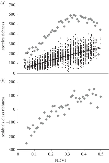
Both grid-cell species richness and NDVI class species richness rise along the NDVI gradient (figure 3a). When controlling for spatial autocorrelation, grid-cell species richness increases monotonically with NDVI (r2=0.483,
F1,1856=57.93,p⬍0.001) and a squared term of NDVI is not significant (F1,1855=1.92, n.s.). However, NDVI class species richness shows a marked hump-shaped relation-ship (r2=0.85, n=47, p⬍0.001) reaching a ceiling at high but not the highest NDVI levels; the removal of the squared term results in a significant decrease in the model fit (Fchange 1,46=89.15,p⬍0.001).
(b) Species richness and area
Maximum geographical extent and surface area of the NDVI classes correlate with NDVI class species richness (log–log transformation, n=46: r2
extent=0.38, p⬍0.001;
r2
1688 A. Bonn and others Structure of species–energy relationship
700
600
500
400
300
200
100
0
200
100
0
–200 –100
–300
0 0.1 0.2 0.3 0.4 0.5 NDVI
residuals class richness
species richness
(a)
(b)
Figure 3. (a) Patterns of species richness along the NDVI gradient for grid-cell species richness (black squares, regression lines are given for linear and unimodal relationship) and for NDVI class species richness (diamonds). (b) Controlling for log surface area and log geographical extent reveals a more linear relationship between NDVI and NDVI class richness (unstandardized residuals plotted).
relationship into a more linear increase (r2=0.85,n=46,
p⬍0.001; although inclusion of the squared term still provides a better model fit, there is no significant internal maximum: Fchange 1,41=84.25, p⬍0.001; figure 3b). Therefore, the strong hump-shaped relationship is an arte-fact of the wider coverage of intermediate levels of energy in South Africa (see figure 1), which consequently sample more species ranges. Not surprisingly, mean grid-cell species richness is only weakly affected by the two cover-age parameters of the respective NDVI class (log–log transformation,n=46:r2
extent=0.09,p⬍0.05;rarea2 =0.02, n.s.), and the relationship between NDVI and mean grid-cell species richness is not altered when controlling for both (r2=0.89,n=46,p⬍0.001).
(c) Energy ranges and geographical ranges along the energy gradient
The mean energy range of species, i.e. the range of occupied NDVI classes, decreases with increasing NDVI, both when assessed for the species occurring in individual grid cells (r2=0.37, n=1858, p⬍0.001) and for the species occurring in individual NDVI classes (r2=0.95,
n=47, p⬍0.001; figure 4a). The same is true for the mean geographical range of species occurring in individual
Proc. R. Soc. Lond.B (2004)
0.55
0.50
0.45
0.40
0.35
0.30
0.25
0.20 1600
1400
1200
1000
800
600
400
200
0 180
160
140
120
100
80
60
40
20
0 0.1 0.2 0.3 0.4 0.5 NDVI
mean energy range
mean geographical range
NDVI class species richness
700
600
500
400
300
200
100
0 700
600
500
400
300
200
100
0
species richness
species richness
(a)
(b)
(c)
Figure 4. (a) Mean energy range and (b) mean geographical range of species present in NDVI classes along the
productivity gradient (squares; error bars indicate s.d.). In (a,b) the overall NDVI class species-richness curve is given for comparison (diamonds). (c) Variation of patterns of NDVI class species richness for geographical RSQs along the NDVI gradient (RSQ: first, grey triangles; second, circles; third, squares; fourth, open triangles).
grid cells (r2=0.49,n=1858, p⬍0.001), and for those occurring in individual NDVI classes (r2=0.96, n=47,
p⬍0.001; figure 4b). Therefore, species present at higher levels of energy tend to be more restricted in both their distribution across energy levels and their distribution across space. Most rare species actually occur only at high NDVI levels (figure 4c).
(d) Energy–occupancy relationship
[image:5.598.57.280.61.395.2]80
70
60
50
40
30
20
10
0
25
20
15
10
5 0
–5
–10
–15
25
20
15
10
5
0
40
35
30
25
20
15
10
5
0 –20
0.1 0.2 0.3 0.4 0.5
NDVI
mean reporting rate (%)
(presence records)
mean occupanc
y (%)
residuals mean occupanc
y (%)
mean reporting rate (%)
(all records)
(a)
(b)
(c)
(d)
levels. This pattern holds for all geographical range size quartiles, but is weaker for narrowly distributed species (figure 5a). Also, the pattern changes from a monotonic increase for common species (r2
fourth=0.80, n=43,
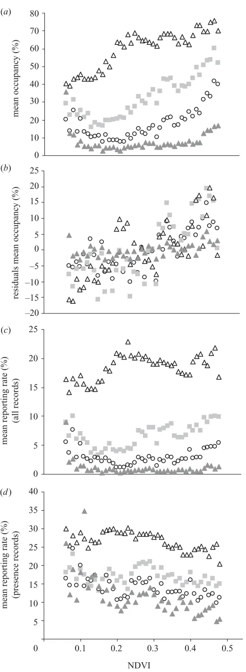
Figure 5. (a) Mean percentage occupancy of species along the productivity gradient; (b) controlled for log geographical extent and log surface area (unstandardized residuals plotted). Average mean species reporting rate for: (c) all grid cells within NDVI classes; and (d) only occupied grid cells within NDVI classes along the NDVI gradient (RSQ: first, grey triangles; second, circles; third, squares; fourth, open triangles).
p⬍0.001) to a significantly negative hump-shaped pat-tern with an initial decrease for all other species (first to third RSQ: r2
first=0.50, rsecond2 =0.88, rthird2 =0.88; all
n=43, p⬍0.001). As intermediate levels of NDVI are
more widely scattered (figure 2), mean percentage occu-pancy is expected to be lower in these areas, assuming approximately contiguous geographical ranges of species. Indeed, controlling simultaneously for geographical extent and surface area by partial correlations reveals strong lin-ear relationships between NDVI and residuals of mean percentage occupancy for all species (figure 5b; r2
first
=0.10, p⬍0.05; r2
second=0.69, p⬍0.001; rthird2 =0.83,
p⬍0.001;r2
fourth=0.66,p⬍0.001; alln=43).
In fact, on a single species evaluation, the majority (80%) of species show increasing occupancies along the energy gradient, with significantly positive correlations between NDVI and occupancy for 64% of all species.
(e) Energy–abundance relationship
The increase in species occupancy is parallelled by an overall increase in species average reporting rates within NDVI classes, a proxy measure for abundance (figure 5c). The pattern mimics that of occupancy (monotonic increase fourth RSQ:r2
fourth=0.28; negative hump-shaped relationship for first to third RSQ: r2
first=0.37, rsecond2
=0.62, r2
third=0.55; all n=43, p⬍0.001) as there are strong linear correlations between mean percentage occu-pancy and average reporting rate (first to fourth RSQ: r2
first=0.59, rsecond2 =0.52, rthird2 =0.65, rfourth2 =0.30; all
n=43,p⬍0.001).
By contrast, when analysing only those grid cells with presence records within NDVI classes, the average reporting rate per species actually decreases along the NDVI gradient (figure 5d; first to fourth RSQ, alln=43:
r2
first=0.46, p⬍0.001; rsecond2 =0.35, p⬍0.001; rthird2
=0.08, n.s.;r2
fourth=0.40,p⬍0.001). Also for single spe-cies evaluations, significant correlations between the mean reporting rate per occurrence record within NDVI classes and NDVI are negative for 34% of all species and positive for only 19%. The ratio of negative to positive correlations is similar for all quartiles with a slightly higher proportion of negative correlations for narrow ranging species (percentage of negative versus percentage of positive cor-relations at p⬎0.05, first to fourth RSQ: 20/4, 35/18, 36/25, 41/30).
(f) Species turnover
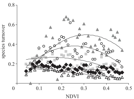
Overall species turnover between adjacent grid cells within individual NDVI classes decreases linearly along the energy gradient (figure 6; r2=0.35, n=43,
[image:6.598.51.292.56.714.2]1690 A. Bonn and others Structure of species–energy relationship
0.8
0.6
0.4
0.2
0 0.1 0.2 0.3 0.4 0.5
NDVI
[image:7.598.55.286.58.229.2]species turnover
Figure 6. Relative species turnover (sim) between adjacent
grid cells within NDVI classes along the productivity gradient (all species, diamonds; RSQ: first, grey triangles; second, circles; third, squares; fourth, open triangles; regression lines follow the sequence RSQ first, second, third, all species, fourth from top to bottom).
Along the energy gradient, for the first, second and third RSQ species, turnover shows a hump-shaped pattern (first to third RSQ: r2
first=0.30, n=35 ; rsecond2 =0.33, n=42;
r2
third=0.44, n=43; all p⬍0.001). The wider the distri-bution of species, the earlier the decrease phase in turn-over along the energy gradient. In the extreme, the turnover of common species decreases monotonically along the whole gradient (r2=0.63,n=43,p⬍0.001), as all species are present in most NDVI classes and percent-age occupancy rises continuously (figures 4cand 5a,b).
4. DISCUSSION
At a quarter-degree resolution, the species richness of South African birds increases monotonically with energy availability across a considerable range of NDVI values (figure 3a,b). This is in accord with the findings of Van Rensburget al.(2002), and those of similar studies of sev-eral other assemblages (Waide et al. 1999; Mittelbach et al. 2001). Within South Africa, the monotonic increase of avian species richness with energy at a quarter-degree resolution is not a by-product of more productive areas having a greater geographical extent (cf. Rosenzweig 1995), because the most productive and species-rich regions are less extensive than those of intermediate pro-ductivity, and the effect of productivity is even stronger after controlling for the variation in area.
The marked increase in species occupancy along the energy gradient indicates that factors affecting the pres-ence or maintenance of populations of individual species influence the observed patterns of species richness. This conclusion is supported by the fact that most species can be found in very productive areas, and species occurring in areas of low productivity are mostly those that occur everywhere, as indicated by the relationship between pro-ductivity and range size (figure 4a,b). This supports the importance of ecological factors independently affecting each species, rather than evolutionary processes respon-sible for the evolution of whole assemblages (see § 1). Although there are also rare species that only occupy less
Proc. R. Soc. Lond.B (2004)
productive areas, they do not form a separate species pool, and energy levels seem to affect most species in a simi-lar way.
The increase of species occupancy with increasing energy (figure 5a) is probably responsible for the generally decreasing trend of species turnover along the productivity gradient (figure 6), as grid cells become more and more similar to each other. The concept of elevated species turnover accounting for increased species richness at larger scales (Whittaker 1960; Gaston & Williams 1996; Brown & Lomolino 1998) is therefore not appropriate here. Previous findings of positive relationships between species richness and turnover might have been confused by using traditional measures of beta diversity confounded by species richness itself (Koleff et al. 2003). Using the
sim index, a similar decrease in overall species turnover along species-richness gradients was also observed by Len-nonet al.(2001), who attributed it to more random mix-tures of rarer species within areas of low species richness. All of these findings can be considered as providing sup-port for the ‘more individuals’ hypothesis. However, this hypothesis also predicts higher densities of all species in grid cells of higher available energy, which we did not observe. On the contrary, we documented a decrease of mean species abundance with increasing productivity, as measured by mean reporting rate within occupied grid cells (figure 5d). Although results for RSQs must be inter-preted with caution, as reporting rates are not fully compa-rable among species, the trends are similar for all species of differing range sizes. This decrease in local population density along the productivity gradient could result from reductions in niche breadth and/or higher diversity or het-erogeneity of resources within grid cells (figure 1d; i.e. lower amounts of each individual resource). If this is the case, then both the ‘more individuals’ and the ‘specializa-tion’ hypotheses may be relevant, but on different spatial scales. It seems that rather than simple increases in the amounts of all resources, increases in energy availability increase the probability of occurrence of different resources necessary for the occurrence of different species. Our findings therefore indicate that ecological processes responsible for establishment and maintenance of local populations are also responsible for the observed species– energy relationship on this spatial scale. It is probable that evolutionary processes of speciation, diversification and differential extinction are more important on larger spatial scales, and that hump-shaped species–energy relationships as documented for the whole of Africa (Balmford et al. 2001) may concern different species pools with different rates of evolution. But we predict that whenever the species–energy relationship concerns essentially one com-mon species pool, ecological factors related to population probability of occurrence and maintenance will be important and species richness will therefore increase monotonically with productivity.
Service (grant no. D/01/05749), the GA AV CR (grant no. KJB619740) and the Leverhulme Trust (grant no. 20010273).
REFERENCES
Abrams, P. A. 1995 Monotonic or unimodal diversity– productivity gradients, what does competition theory pre-dict?Ecology76, 2019–2027.
Allen, A. P., Brown, J. H. & Gillooly, J. F. 2002 Global biodiv-ersity, biochemical kinetics, and the energetic–equivalence rule.Science297, 1545–1548.
Balmford, A., Moore, J. L., Brooks, T., Burgess, N., Hansen, L. A., Williams, P. & Rahbek, C. 2001 Conservation con-flicts across Africa.Science291, 2616–2619.
Brown, J. H. & Lomolino, M. V. 1998Biogeography. Oxford: Blackwell Science.
Chase, J. M. & Leibold, M. A. 2002 Spatial scale dictates the productivity–biodiversity relationship.Nature416, 427–429. Currie, D. 1991 Energy and large-scale patterns of animal- and
plant-species richness.Am. Nat.137, 27–49.
Gaston, K. J. 2000 Global patterns in biodiversity.Nature405, 220–227.
Gaston, K. J. & Blackburn, T. M. 1999 A critique of macro-ecology.Oikos84, 353–368.
Gaston, K. J. & Williams, P. H. 1996 Spatial patterns in taxo-nomic diversity. InBiodiversity: a biology of numbers and dif-ference (ed. K. J. Gaston), pp. 202–229. Oxford: Blackwell Science.
Harrison, J. A., Allan, D. G., Underhill, L. G., Herremans, M., Tree, A. J., Parker, V. & Brown, C. J. 1997The atlas of Southern African birds. Johannesburg: BirdLife South Africa. Hurlbert, A. H. & Haskell, J. P. 2003 The effect of energy and seasonality on avian species richness and community compo-sition.Am. Nat.161, 83–97.
Kaspari, M., O’Donnell, S. & Kercher, J. R. 2000 Energy, den-sity, and constraints to species richness: ant assemblages along a productivity gradient.Am. Nat.155, 280–293. Kaspari, M., Yuan, M. & Alonso, L. 2003 Spatial grain and
the causes of regional diversity gradients in ants.Am. Nat.
161, 459–477.
Kerr, J. T. & Packer, L. 1997 Habitat heterogeneity as a deter-minant of mammal species richness in high-energy regions.
Nature385, 252–254.
Kerr, J. T., Southwood, T. R. E. & Cihlar, J. 2001 Remotely sensed habitat diversity predicts butterfly species richness and community similarity in Canada. Proc. Natl Acad. Sci. USA98, 11 365–11 370.
Koleff, P., Gaston, K. J. & Lennon, J. J. 2003 Measuring beta diversity for presence–absence data. J. Anim. Ecol. 72, 367–382.
Lennon, J. J., Koleff, P., Greenwood, J. J. D. & Gaston, K. J. 2001 The geographical structure of British bird distri-butions: diversity, spatial turnover and scale.J. Anim. Ecol.
70, 966–979.
Littell, R. C., Milliken, G. A., Stroup, W. W. & Wolfinger, R. D. 1996 SAS system for mixed models. Cary, NC: SAS Institute Inc.
Mitchell-Olds, T. & Shaw, R. G. 1987 Regression analysis of natural selection: statistical inference and biological interpretation.Evolution41, 1149–1161.
Mittelbach, G. G., Steiner, C. F., Scheiner, S. M., Gross, K. L., Reynolds, H. L., Waide, R. B., Willig, M. R., Dod-son, S. I. & Gough, L. 2001 What is the observed relation-ship between species richness and productivity?Ecology82, 2381–2396.
Robertson, A., Simmons, R. E., Jarvis, A. M. & Brown, C. J. 1995 Can bird atlas data be used to estimate population-size? A case study using Namibian endemics.Biol. Conserv.
71, 87–95.
Rohde, K. 1997 The larger area of the tropics does not explain the latitudinal gradient in species diversity.Oikos79, 169–172. Rosenzweig, M. L. 1995 Species diversity in space and time.
Cambridge University Press.
Rosenzweig, M. L. & Abramsky, Z. 1993 How are diversity and productivity related? InSpecies diversity in ecological com-munities(ed. R. E. Ricklefs & D. Schluter), pp. 52–65. Uni-versity of Chicago Press.
Rosenzweig, M. L. & Sandlin, E. A. 1997 Species diversities and latitudes: listening to area’s signal.Oikos80, 172–176. Srivastava, D. S. & Lawton, J. H. 1998 Why more productive sites have more species: an experimental test of theory using tree-hole communities.Am. Nat.152, 510–529.
Storch, D. 2003 Comment on ‘global biodiversity, biochemical kinetics, and the energetic-equivalence rule’. Science 299, 346b.
Turner, J. R. G., Lennon, J. J. & Lawrenson, J. A. 1988 British bird species distribution and energy theory. Nature 335, 539–541.
Van Rensburg, B. J., Chown, S. L. & Gaston, K. J. 2002 Species richness, environmental correlates, and spatial scale: a test using South Africa.Am. Nat.159, 566–577. Waide, R. B., Willig, M. R., Steiner, C. F., Mittelbach, G.,
Gough, L., Dodson, S. I., Juday, G. P. & Parmenter, R. 1999 The relationship between productivity and species richness.A. Rev. Ecol. Syst.30, 257–300.
Whittaker, R. J. 1960 Vegetation of the Siskiyou Mountains, Oregon and California.Ecol. Monogr.30, 279–338. Whittaker, R. J., Willis, K. J. & Field, R. 2001 Scale and
spe-cies richness: towards a general, hierarchical theory of spec-ies diversity.J. Biogeogr.28, 453–470.
Woodward, F. I., Lomas, M. R. & Lee, S. E. 2001 Predicting the future production and distribution of global terrestrial vegetation. In Terrestrial global productivity (ed. J. Roy, B. Saugier & H. Mooney), pp. 519–539. London: Academic. Wright, D. H. 1983 Species–energy theory: an extension of
species area theory.Oikos41, 496–506.