Do the methods used to analyse missing data really matter? An examination of data from an observational study of Intermediate Care patients

R E S E A R C H A R T I C L E

Open Access

Do the methods used to analyse missing data

really matter? An examination of data from an

observational study of Intermediate Care patients

Billingsley Kaambwa

, Stirling Bryan

and Lucinda Billingham

Abstract

Background:Missing data is a common statistical problem in healthcare datasets from populations of older people. Some argue that arbitrarily assuming the mechanism responsible for the missingness and therefore the method for dealing with this missingness is not the best option—but is this always true? This paper explores what happens when extra information that suggests that a particular mechanism is responsible for missing data is disregarded and methods for dealing with the missing data are chosen arbitrarily.

Regression models based on 2,533 intermediate care (IC) patients from the largest evaluation of IC done and published in the UK to date were used to explain variation in costs, EQ-5D and Barthel index. Three methods for dealing with missingness were utilised, each assuming a different mechanism as being responsible for the missing data: complete case analysis (assuming missing completely at random—MCAR), multiple imputation (assuming missing at random—MAR) and Heckman selection model (assuming missing not at random—MNAR). Differences in results were gauged by examining the signs of coefficients as well as the sizes of both coefficients and associated standard errors.

Results:Extra information strongly suggested that missing cost data were MCAR. The results show that MCAR and MAR-based methods yielded similar results with sizes of most coefficients and standard errors differing by less than 3.4% while those based on MNAR-methods were statistically different (up to 730% bigger). Significant variables in all regression models also had the same direction of influence on costs. All three mechanisms of missingness were shown to be potential causes of the missing EQ-5D and Barthel data. The method chosen to deal with missing data did not seem to have any significant effect on the results for these data as they led to broadly similar conclusions with sizes of coefficients and standard errors differing by less than 54% and 322%, respectively.

Conclusions:Arbitrary selection of methods to deal with missing data should be avoided. Using extra information gathered during the data collection exercise about the cause of missingness to guide this selection would be more appropriate.

Keywords:Missing data, Complete case analysis, Multiple imputation, Generalised linear model, Heckman selection, Observational data

Background

Missing data is an unwanted reality in most evaluations of services for older people as it can lead to biased results as well as threats to the generalisability and power of the results obtained from analysing such data [1, 2]. Even under the best of conditions, missing data

may result in a significant reduction in sample size lead-ing to threats to external validity as a sample reduced in size may no longer be representative of the target popu-lation [3–5]. This is more problematic in circumstances where the likelihood of response is related to observed characteristics. Certain forms of missingness can reduce the statistical power of the analyses of the available data and therefore compromise the internal validity of a study, which is more serious [3, 6, 7]. A situation that can potentially lead to reduced statistical power is when * Correspondence:[email protected]

1

Health Economics Unit, Public Health Building, University of Birmingham, Edgbaston, Birmingham B15 2TT, United Kingdom

Full list of author information is available at the end of the article

the probability of response is associated with the values of the variable for which values are only partly observed, which is a possibility in a lot of cases [8].

The three main mechanisms that lead to missing data are: missing completely at random (MCAR), missing at random (MAR) and missing not at random (MNAR). If data are MAR or MCAR, they can also be referred to as

“ignorable” data while those MNAR are “non-ignorable” [8]. Missing data are said to be ignorable if the para-meters that are used to model the missing data process are not related to the parameters used to model the observed data while non-ignorability exists if there is a systematic difference between responders and nonre-sponders even after accounting for all the observed data [7, 9]. There are various methods that have been pro-posed to deal with missing data with each of these meth-ods premised on a specific missing data mechanism [1, 10, 11]. Croninger and Douglas [7] indicate that the choice of method used for coping with missing data is not crucial if there is not much missing data and/or the sample is big. This is because most methods will yield similar results in such circumstances. But as the level of missingness rises and/or the sample becomes smaller, the choice of method becomes potentially more signifi-cant. In this paper, we do not provide a detailed discus-sion of the various methods that can be used to deal with missing data. Interested readers can see Fielding et al. [12] for such a discussion. In general though, complete case analysis (both listwise and pairwise dele-tion) can be performed when data are MCAR [13]. Approaches for use when data are MAR include listwise deletion, various imputation techniques, propensity ad-justment strategy, raw maximum likelihood and expect-ation maximisexpect-ation [1, 3, 6, 14]. When data are MNAR, panel selection models, including the Heckman, and pattern-mixture approaches can be used [15–17].

Most times, the method chosen to deal with missing data is not based on concrete evidence of the mechan-ism responsible for this missing data. It is consequently difficult to assess the accuracy of such methods because the data are by definition ‘missing’ [12]. It is a recog-nised fact that data often provide little or no information at all to help determine the correct mechanism behind missingness [3, 18]. In many scenarios, therefore, it is difficult, or even impossible, to know what mechanism is responsible for the missingness. Sometimes more than one mechanism may be responsible for different sets of missing data within the same evaluation [7, 19]. This therefore means that choosing among these alternative methods is not an easy task.

Curran et al. [19] suggest two approaches for deter-mining the missing data mechanism: (1) hypothesis test-ing and (2) collecttest-ing extra information, durtest-ing the data collection process, about why missing data is missing. In

the absence of missing data being recovered and ana-lysed, hypothesis testing can at best only rule out that missing data are MCAR with no way of confirming that data are actually MCAR [20]. Provided enough data has been collected, it therefore seems that, where missing data is irrecoverable, it is only the latter approach that will give some fairly credible indication about whether data are MCAR, MAR or MNAR [8, 19].

This study explores what happens when extra informa-tion that suggests that a particular mechanism is respon-sible for missing data is disregarded and methods for dealing with the missing data are chosen arbitrarily. A dataset from the largest evaluation of intermediate care services done and published in the UK to date is used [21]. Intermediate services (IC) are tailored to prevent admission to acute care or long-term care and also aid discharge from hospital for older people [21]. It is not usual practice for such extra information to be gathered as part of the data collection process in a evaluation such as that for IC and the presence of this information therefore presented a unique opportunity to empirically compare different methods for dealing with missing data. As far as we are aware, this is the first time that this sort of analysis has been done on a dataset of older people in the UK. Using this dataset, which had missing data on several variables, the factors that explain vari-ation in costs per patient, change in EQ-5D from admis-sion to discharge (ΔEQ-5D) and change in the Barthel index from admission to discharge (ΔBarthel) of IC patients were explored in a regression modelling frame-work. These factors could be broadly divided into three groups: IC episode characteristics, descriptors of IC ser-vices and descriptors of IC-related serser-vices. Three meth-ods incorporating techniques for dealing with missing data were used: (1) generalised linear models (GLMs) and ordinary least squares (OLS) on complete cases (as-suming that missing data were MCAR), (2) GLM and OLS models on data obtained through multiple imput-ation (MI) (assuming missing data were MAR) and (3) Heckman selection models (assuming that missing data were MNAR). We were interested in examining the signs of coefficients as well as the sizes of both coeffi-cients and associated standard errors in the regression model results obtained.

Methods

Source of data

evaluation team. Service staff completed study pro forma, with or on behalf of their patients, at the point of admission to the service, for all IC admissions over a defined period. They completed discharge questions on the day of discharge, transfer to another IC service or as soon as possible following end of service provision. In addition, extra information on the reasons as to why some data were missing was obtained from IC coordina-tors, ICNET researchers’ observations as well as from preliminary statistical analyses done on the ICNET data-set [21–23]. Data were collected between January 2003 and January 2004. Ethical approval was granted by the Trent Multicentre Research Ethics Committee.

Missing data in the ICNET dataset

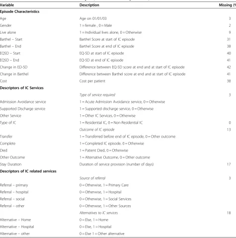
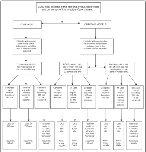
The variables that were collected in the ICNET dataset, based on a sample of 2,253 patients, are presented in Table 1. Up to 42% of the data were missing for some variables in that dataset. Extra information about why data were missing were available for all dependent vari-ables (cost per patient, ΔEQ-5D and ΔBarthel) but not available for nearly all of the independent variables. Be-cause of this lack of information and for purposes of comparing the methods for dealing with missing data, a decision was made to focus on missingness only in the dependent variables. Therefore, 1,536 out of 2,253 obser-vations were excluded from the analyses reported in this paper due to missing values in the independent vari-ables. There was therefore no missing value for all inde-pendent variables (and interaction terms generated using these variables) used in the analyses. A flow chart show-ing how the samples used in the final regression models were arrived at is shown in Figure 1. A sample of 717 individuals was therefore used for the cost per patient models and 125 (17.4%) of these individuals had missing observations on the cost variable. For the ΔEQ-5D and ΔBarthel models, a sample of 1105 individuals was uti-lised. Of this sample, 417 (37.7%) and 392 (35.5%) had missing values on the ΔEQ-5D and ΔBarthel variables, respectively.

The dependent variables

The cost per patient variable was calculated by combin-ing resource data with budget information for the indi-vidual IC services.

The EQ-5D is an outcome measure whose construct validity when used on populations of older people has been well documented [24–26]. It is comprised of five dimensions of health: mobility, self-care, usual activities, pain/discomfort, and anxiety/depression. There are three levels of impairment in each domain: no, some/moder-ate, and extreme problems in the relevant dimension of health. Using these responses, the EQ-5D is able to dis-tinguish between 243 states of health [27, 28]. The

UK-specific EQ-5D valuation algorithm was used in order to convert the EQ-5D health description into a valuation. EQ-5D scores have a range of−0.59 to 1: the maximum score of 1 represents perfect health and a score of 0 represents death [28]. Scores less than 0 represent health states that are worse than death [28–30]. Its generic na-ture makes it comparable across patient populations.

The Barthel Index (BI) is a non-utility based conven-tional clinical scale of funcconven-tional independence which has been recommended by the Royal College of Physi-cians for routine use in the assessment of older people [31]. Its validity when used on a general population of older people has also been shown [32] . To measure a person’s level of functional independence, the BI uses 10 items, with each item carrying different weights [33]. Two items (bathing and grooming) are rated on a two-point scale of 0 and 5, six (feeding, dressing, bowels, bladder, toilet use and stairs) on a three-point scale of 0, 5 and 10 and the last two items (transfers and mobility) are rated on a four-point scale of 0, 5, 10 and 15. The scores on each item are added to produce an overall score which ranges from 0 to 100. To standardise them, the overall scores used in this paper were divided by 5 and therefore ranged from 0 to 20 [34]. The higher the score recorded for an item, the greater the level of inde-pendence. The reliability, sensitivity and suitability for proxy-assessment of the BI has been shown elsewhere [33–35].

Reasons for missing data in the ICNET dataset

When data are MCAR, it implies that the probability of an item missing is unrelated to any measured or un-measured characteristic for that unit [36], while under MAR, the probability of an item having incomplete data depends on other variables in the dataset [1]. MNAR is when the probability of missingness depends on the values of the unobserved values perhaps in addition to one or more other variables and/or the observed vari-ables [37].

Because of time constraints placed on the data collec-tion process, it was not possible to collect all of the cost data. No other reason was established as being respon-sible for the missing cost data. This suggests that where cost data were missing, it would be reasonable to assume that these data were MCAR.

In terms of the missing data on the EQ-5D and Barthel, all three mechanisms (MCAR, MAR and MNAR) could be assumed as the reason for this missingness.

that it was plausible to assume that the missingness mechanism for such data was MCAR.

Secondly, the ΔEQ-5D and ΔBarthel scores were cal-culated by subtracting the scores at admission from those at discharge. A number of individuals had however been transferred to other services before the end of their IC episode. For some of these, it meant that their EQ-5D and Barthel scores at ‘discharge’ were not collected

making it impossible to compute the ΔEQ-5D and

ΔBarthel variables. This could be seen as a situation where the missing data were MAR as the reason for the

patients transfer was more often than not linked to their health or functional status e.g. the more functionally in-dependent an individual was, the more likely they were to be transferred to a less intensive form of IC. Add-itional statistical analyses on the IC dataset [23] also revealed that the Barthel scores were predictive of the missing EQ-5D values, further reinforcing the plausibil-ity of the missing EQ-5D data being MAR.

Thirdly, the mean Barthel scores for some individuals who had missing EQ-5D scores were on average lower than those for individuals who did not have missing EQ-Table 1 Variables for use in economic analysis (with level of completeness)

Variable Description Missing (%)

Episode Characteristics

Age Age on 01/01/03 3

Gender 1 = female , 0 = Male 2

Live alone 1 = Individual lives alone, 0 = Otherwise 9

Barthel–Start Barthel Score at start of IC episode 31

Barthel–End Barthel Score at end of IC episode 38

EQ5D–Start EQ-5D at start of IC episode 40

EQ5D–End EQ-5D at end of IC episode 41

Change in ED-5D Difference between EQ-5D score at end and at start of IC episode 42

Change in Barthel Difference between Barthel score at end and at start of IC episode 41

Cost Cost per patient 38

Descriptors of IC Services

Type of service required 3

Admission Avoidance service 1 = Acute Admission Avoidance service, 0 = Otherwise

Supported Discharge service 1 = Supported discharge service, 0 = Otherwise

Other Service 1 = Other IC Services, 0 = Otherwise

Type of IC 1 = Residential IC, 0 = Non-Residential IC 0

Outcome of IC episode 13

Transfer 1 = Transferred before end of IC episode, 0 = Other outcome

Complete 1 = Completed IC episode, 0 = Otherwise

Died 1 = Patient Died, 0 = Otherwise

Other Outcome 1 = Alternative Outcome, 0 = Other outcome

Stay Duration Duration of service provision (number of days) 17

Descriptors of IC related services

Source of referral 3

Referral–primary 0 = Otherwise, 1 = Primary Care

Referral–hospital 0 = Otherwise, 1 = Hospital

Referral–social 0 = Otherwise, 1 = Social Services

Referral–other 0 = Otherwise, 1 = Other Sources

Alternatives to IC services 18

Alternative–Home 0 = Else, 1 = Home

Alternative–Hospital 0 = Else, 1 = Hospital

5D information [22]. Since some individuals with missing EQ-5D data were associated with lower Barthel scores, it means that, by virtue of the positive relationship between the two instruments [23], there is a possibility that these individuals would also have had lower EQ-5D scores had these been collected. It was therefore reasonable to as-sume that some of the missing data on the EQ-5D could also have been MNAR i.e. the poorer ones’ health status was, the more difficult it was for them to provide data on

the EQ-5D. By the same token, some of the missing Barthel data could have been MNAR.

Choice of regression families

In this exercise, it was important to compare both the signs and sizes of coefficients (and sizes of associated standard errors) from the different regression models. Both costs per patient and outcome variables were skewed and heteroscedastic in their residuals. We chose the GLM

2,253 obs/ patients in the ‘National evaluation of costs

COST MODEL OUTCOME MODELS

1,536 obs with missing data on any of the independent variables used in the cost model

excluded

717 obs of which 125 had missing data on the cost variable only

Complete case analysis based on 592 obs Selection model assuming 125 obs to be censored MI used to impute missing costs for 125 patients GLM on 592 obs Assuming MCAR GLM on 717 obs Assuming MAR Heckman model on 717 obs, of which 125 were ‘censored’ Assuming MNAR

EQ-5D model: 1,105 obs of which 417 had

missing data on the EQ-5D variable only

1,148 obs with missing data on any of the independent

variables used in the outcome models excluded

Barthel model: 1,105 obs of which 392 had

missing data on the Barthel variable only

OLS on 688 obs Assu-ming MCAR OLS on 1,105 obs Assu-ming MAR Heckman model on 1,105 obs, of which 417 were ‘censored’ Assuming MNAR OLS on 713 obs Assu-ming MCAR OLS on 1,105 obs Assu-ming MAR Heckman model on 1,105 obs, of which 392 were ‘censored’ Assuming MNAR Complete case analysis based on 713 obs MI used to impute EQ-5D scores for 417 patients Selection model assuming 417 obs to be censored Complete case analysis based on 688 obs MI used to impute missing Barthel scores for 392 patients Selection model assuming 392 obs to be censored

and out comes of Intermediate Care’ dataset

as it is able to simultaneously deal with both problems [38, 39]. We also used log-transformation where the natural log of the dependent variable was obtained [40] as another method for dealing with the skewed cost data despite sev-eral limitations associated with this approach [41, 42]. For the cost models, therefore, a decision was made for the GLM to be used for both the complete cases and the multiply imputed datasets while a log transformed cost per patient was used in the Heckman regression model. As the exponentiated coefficients from the GLM model have been shown to be easily comparable to the exponen-tiated counterparts obtained from a log-transformed model [43], the results of all the cost per patient models are presented in terms of exponentiated coefficients.

A different approach was taken for the health-outcome dependent variables (ΔEQ-5D and ΔBarthel). This was because these variables also had negative values. As a result, log transformation of these variables would have required the use of a shift factor and the transformed variables would then have had to be appro-priately retransformed once the results of the model had been obtained. However for ease of analysis and com-parison, a decision was made to use the raw scale of these variables. As a result, OLS regressions were used for both the ΔEQ-5D and ΔBarthel in the regression on complete cases and on multiply imputed datasets. Fur-ther, OLS regressions on a raw scale have also been widely used for modelling such outcome data in the lit-erature [44]. The raw scale of the two variables was also used in the Heckman selection models.

Approaches for dealing with the missing data

For our two samples (n = 717 and n = 1,105) obtained from the ICNET dataset, three methods, each assuming either MCAR, MAR or MNAR, were used. A regression framework was employed in the analysis and in general, the regression relationship between the outcomes of interest and the independent variables could be illu-strated as [45]:

Yi¼β0þβ1iþ. . .þβkþXkiþμi

where Yi denotes the outcome of interest (cost per pa-tient,ΔEQ-5D orΔBarthel) for the ith individual,β_i. . ._k are the coefficients,Xi. . ._kare the explanatory variables (both single and interaction terms) for the ith individual andμ_iis the stochastic error term for the ith individual.

A total of six sets of regression models (two for each method) were conducted:

Method 1 involved running regression models on complete cases (assuming that data were MCAR). A GLM was used to explain variation in‘cost per patient’ while OLS models were run for cases where the dependent variables wereΔEQ-5D andΔBarthel.

Pairwise deletion, implying the use of all available data on the particular variables specified in each model, was the method used to arrive at the samples modelled as complete cases, As a result, disparate sample sizes of 592, 688 and 713 observations for the cost per patient, ΔEQ-5D andΔBarthel models, respectively, were used (please see Figure1).

Method 2 involved running GLM and OLS regression models again to explain variation in costs per patient and outcomes (ΔEQ-5D andΔBarthel), respectively. Here, however, we used multiply imputed datasets (assuming that data were MAR) based on a multivariate normal model. [1] Up to about 38% of the data were missing and multiply imputed datasets were created to account for these missing data before running GLM and OLS regression models. These analyses focussed on imputing values for the dependent variables where the

independent variables were not missing thereby creating complete datasets i.e. 717 observations for the cost per patient model and 1105 observations for theΔEQ-5D andΔBarthel models. The rationale for this particular imputation was to allow for direct comparison between the results obtained using this method and those produced by method 3 (described below), which comparison required that essentially the same samples were analysed. Five sets of imputations were created following conventional practice [11]. Since there was up to 38% data missing, these imputations led to point estimates that were at least (1 + 0.38/5)−1= 93% as efficient as those based on m =∞imputations [1]. In method 3, Heckman selection models (assuming that missing data were MNAR) were run on the log of

‘cost per patient’, onΔEQ-5D andΔBarthel using

‘complete cases’. Whereas method 1 only considered cases where there was no missing data for both the dependent variable and independent variables, method 3 considers all subjects including those that had missing cost, EQ-5D or Barthel information. The sample selection used a dummy variable equal to 1 if the dependent variable was not missing and equal to 0 if it was. Using this classification, 125 out of 717 observations were censored (missing) for the cost per patient model while 417 and 392, out of 1105 observations, were censored for theΔEQ-5D and ΔBarthel models, respectively.

Multiple imputations were conducted in NORM [46] while the rest of the analyses were done in STATA ver-sion 8.2 [47].

Results

Cost per patient models

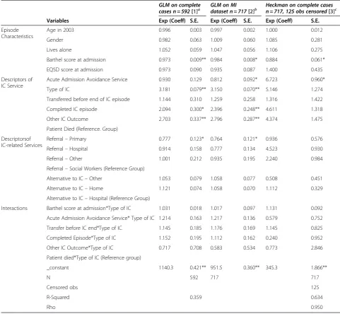
The results of the GLM regression model on complete cases (method 1) and GLM regression model on multi-ply imputed datasets (method 2) are similar. As shown in Table 2, significant predictors of cost per patient were the Barthel score at admission, IC function (acute ad-mission avoidance service or not), type of IC (residential or not), if one completed an IC episode, other IC out-come and if the source of referral was primary care. All of the variables that were found to be significant in method (2) were also significant in method (1) with the exception of one (acute admission avoidance service)

which was significant in model (2) only. Also, the size of coefficients for nearly all of these variables differed by less than 3.4% except the one for‘completed IC episode’ which differed by about 14.4%. The sizes of the standard errors were also similar. Further, the variables significant in both models had the same direction of influence on costs per patient. On the other hand, the results obtained from the Heckman selection regression model (method 3) were much more different. A lot more vari-ables were found to be insignificant with only two variables (Barthel score at admission and acute admis-sion avoidance service) shown to significantly influence Table 2 Comparison of results from three methods of regression analysis of costs per patient

GLM on complete

cases n = 592[1]a GLM on MI_{dataset n = 717[2]}b Heckman on complete cases_{n = 717, 125 obs censored[3]}c

Variables Exp (Coeff) S.E. Exp (Coeff) S.E. Exp (Coeff) S.E.

Episode Characteristics

Age in 2003 0.996 0.003 0.997 0.002 1.000 0.012

Gender 0.982 0.063 1.009 0.060 1.085 0.281

Lives alone 1.052 0.059 1.047 0.056 1.106 0.275

Barthel score at admission 0.973 0.009** 0.984 0.008* 0.884 0.061*

EQ5D score at admission 0.973 0.090 0.935 0.087 1.400 0.435

Descriptors of IC Service

Acute Admission Avoidance Service 0.930 0.129 0.812 0.092* 6.723 0.960*

Type of IC 3.181 0.079** 3.150 0.070** 5.146 1.274

Transferred before end of IC episode 1.144 0.310 1.259 0.258 1.316 1.422

Completed IC episode 2.094 0.300* 2.396 0.248** 4.611 1.318

Other IC Outcome 2.703 0.337** 2.796 0.287** 4.374 1.475

Patient Died (Reference. Group)

Descriptorsof IC-related Services

Referral–Primary 0.777 0.123* 0.764 0.121* 0.936 0.576

Referral–Hospital 0.914 0.158 0.777 0.134 4.523 0.930

Referral–Other 1.001 0.212 0.935 0.195 2.240 0.984

Referral–Social Workers (Reference Group)

Alternative to IC–Other 1.053 0.079 1.058 0.077 0.508 0.451

Alternative to IC–Home 1.121 0.074 1.058 0.070 1.112 0.329

Alternative to IC–Hospital (Reference Group)

Interactions Barthel score at admission*Type of IC 1.031 0.018 1.017 0.097 1.131 0.092

Acute Admission Avoidance Service* Type of IC 1.214 0.163 1.217 0.136 0.579 0.752

Transfer before IC end*Type of IC 1.145 0.185 1.176 0.169 1.145 0.825

Completed Episode*Type of IC 1.152 0.195 1.112 0.162 0.240 0.952

Other IC Outcome*Type of IC 0.717 0.708 0.583 0.534 0.773 2.846

Patient died*Type of IC (Reference group)

_constant 1140.3 0.421** 951.5 0.360** 345.3 1.866**

N 592 717 717

Censored obs 125

R-Squared 0.359 0.634

Rho 0.950

* 5% level of significance, ** 1% level of significance; Dependent variable: cost per patient for GLM and log of cost per patient for Heckman Selection model; IC = Intermediate care;

a

Method 1 assumes that missing data are MCAR;

b

Method 2 assumes that missing data are MAR;c

costs per patient. The sizes of the coefficients in the Heckman model were also different from those of the other two methods. For instance, the coefficient for

‘acute admission avoidance service’was about 730 times bigger than that obtained in method (2). The mills ratios were −3.402 and −4.506 for the Heckman selection models with and without interactions, respectively. These were both statistically significant at 95% level of significance.

Change in EQ-5D models

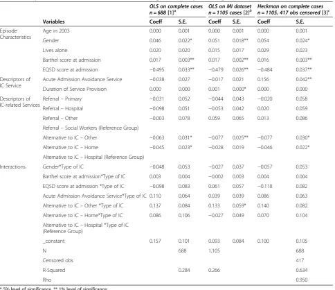
Here, the results from all three models/methods were broadly similar (Table 3). Significant predictors of ΔEQ-5D were gender, Barthel score at admission, EQ-ΔEQ-5D score at admission, IC function, duration of service

provision and likely alternatives were IC not available (home and other alternative). Nearly all of the variables that were significant in one model were also significant in the other models. The only exceptions were the ‘ dur-ation of service provision’ and ‘Alternative to IC-Other *Type of IC’ (both only significant in method 2),‘acute admission avoidance service’(only significant in method 3) and‘alternative to IC-Other’(significant only in mod-els 1 and 3). The sizes of the coefficients of variables commonly significant in all models differed at most by about 22% with the standard errors differing at most by 42% (Table 3). Further, the variables significant in all three models had the same direction of influence on the change in EQ-5D. The mills ratios were −0.284 and

−0.143 for the Heckman selection models with and

Table 3 Comparison of results from three methods of regression analysis (Change in EQ5D)

OLS on complete cases

n = 688[1]a OLS on MI dataset_{n = 1105 cases[2]}b Heckman on complete cases_{n = 1105, 417 obs censored[3]}c

Variables Coeff S.E. Coeff S.E. Coeff S.E.

Episode Characteristics

Age in 2003 0.000 0.001 0.000 0.001 0.000 0.001

Gender 0.046 0.022* 0.051 0.018** 0.054 0.024*

Lives alone 0.020 0.020 0.015 0.017 0.029 0.023

Barthel score at admission 0.017 0.003** 0.017 0.002** 0.016 0.003**

EQ5D score at admission −0.495 0.033** −0.479 0.026** −0.484 0.037**

Descriptors of IC Service

Acute Admission Avoidance Service −0.038 0.027 −0.017 0.021 0.156 0.042**

Duration of Service Provision 0.000 0.000 0.001 0.000* 0.000 0.000

Descriptors of IC-related Services

Referral–Primary −0.031 0.052 −0.044 0.043 −0.020 0.058

Referral–Hospital −0.098 0.051 −0.053 0.042 0.020 0.059

Referral–Other −0.003 0.078 0.059 0.065 0.013 0.086

Referral–Social Workers (Reference Group)

Alternative to IC–Other −0.063 0.031* −0.077 0.025** −0.077 0.030*

Alternative to IC–Home −0.045 0.023* −0.028 0.019 −0.046 0.022*

Alternative to IC–Hospital (Reference Group)

Interactions Gender*Type of IC −0.048 0.053 −0.027 0.037 −0.057 0.053

Barthel score at admission*Type of IC 0.003 0.004 −0.002 0.003 0.004 0.004

EQ5D score at admission *Type of IC −0.098 0.083 0.061 0.057 −0.118 0.082

Acute Admission Avoidance Service*Type of IC 0.110 0.064 0.039 0.039 0.086 0.063

Alternative to IC–Other *Type of IC 0.137 0.084 0.133 0.059* 0.140 0.082

Alternative to IC–Home*Type of IC 0.086 0.106 −0.027 0.049 0.070 0.104

Alternative to IC–Hospital *Type of IC (Reference Group)

_constant 0.157 0.101 0.093 0.084 0.100 0.105

N 688 1,105 688

Censored obs 417

R-Squared 0.284 0.266 0.634

Rho 0.950

* 5% level of significance, ** 1% level of significance; Dependent variable: change in EQ-5D, IC = Intermediate care

a

Method 1 assumes that missing data are MCAR;b

Method 2 assumes that missing data are MAR;c

without interactions, respectively. These were both sta-tistically significant at 95% level of significance.

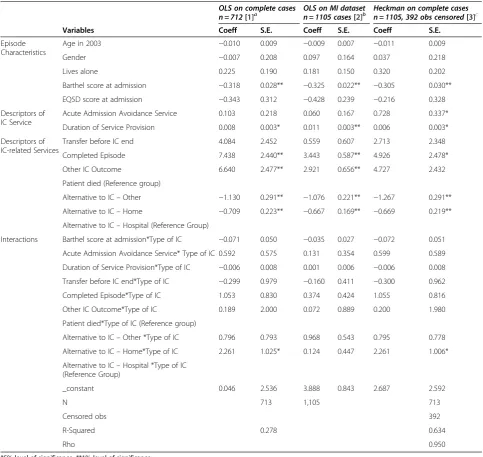
Change in Barthel models

As in the‘change in EQ-5D’models, the results obtained from all three models/methods for the change in Barthel were broadly similar (Table 4). Significant predictors of ΔBarthel were the Barthel score at admission, IC func-tion, outcome of IC episode (completed and other), likely alternatives were IC not available (home and other) and an interaction term between likely alterna-tives were IC not available and type of IC. All of the

variables that were significant in one model were also significant in the other models with the exception of

‘acute admission avoidance service’ and ‘Alternative to IC—Home*Type of IC’ (only significant in method 3) and‘Other IC Outcome’variable only significant in both method (1) and method (2). However, the differences in terms of the sizes of coefficients and standard errors of variables significant in all methods were slightly bigger in these models than in the ‘change in EQ-5D’ models. They differed at most by about 54% and 322% for coeffi-cients and standard errors, respectively. The variables significant in all three models had the same direction of Table 4 Comparison of results from three methods of regression analysis (Change in Barthel)

OLS on complete cases

n = 712[1]a OLS on MI dataset_{n = 1105 cases[2]}b Heckman on complete cases_{n = 1105, 392 obs censored[3]}c

Variables Coeff S.E. Coeff S.E. Coeff S.E.

Episode Characteristics

Age in 2003 −0.010 0.009 −0.009 0.007 −0.011 0.009

Gender −0.007 0.208 0.097 0.164 0.037 0.218

Lives alone 0.225 0.190 0.181 0.150 0.320 0.202

Barthel score at admission −0.318 0.028** −0.325 0.022** −0.305 0.030**

EQ5D score at admission −0.343 0.312 −0.428 0.239 −0.216 0.328

Descriptors of IC Service

Acute Admission Avoidance Service 0.103 0.218 0.060 0.167 0.728 0.337*

Duration of Service Provision 0.008 0.003* 0.011 0.003** 0.006 0.003*

Descriptors of IC-related Services

Transfer before IC end 4.084 2.452 0.559 0.607 2.713 2.348

Completed Episode 7.438 2.440** 3.443 0.587** 4.926 2.478*

Other IC Outcome 6.640 2.477** 2.921 0.656** 4.727 2.432

Patient died (Reference group)

Alternative to IC–Other −1.130 0.291** −1.076 0.221** −1.267 0.291**

Alternative to IC–Home −0.709 0.223** −0.667 0.169** −0.669 0.219**

Alternative to IC–Hospital (Reference Group)

Interactions Barthel score at admission*Type of IC −0.071 0.050 −0.035 0.027 −0.072 0.051

Acute Admission Avoidance Service* Type of IC 0.592 0.575 0.131 0.354 0.599 0.589

Duration of Service Provision*Type of IC −0.006 0.008 0.001 0.006 −0.006 0.008

Transfer before IC end*Type of IC −0.299 0.979 −0.160 0.411 −0.300 0.962

Completed Episode*Type of IC 1.053 0.830 0.374 0.424 1.055 0.816

Other IC Outcome*Type of IC 0.189 2.000 0.072 0.889 0.200 1.980

Patient died*Type of IC (Reference group)

Alternative to IC–Other *Type of IC 0.796 0.793 0.968 0.543 0.795 0.778

Alternative to IC–Home*Type of IC 2.261 1.025* 0.124 0.447 2.261 1.006*

Alternative to IC–Hospital *Type of IC (Reference Group)

_constant 0.046 2.536 3.888 0.843 2.687 2.592

N 713 1,105 713

Censored obs 392

R-Squared 0.278 0.634

Rho 0.950

*5% level of significance, **1% level of significance; Dependent variable: change in Barthel, IC = Intermediate care;

a

Method 1 assumes that missing data are MCAR;b

Method 2 assumes that missing data are MAR;c

influence on the change in Barthel. The mills ratios were

−1.662 and −0.101 for the Heckman selection models with and without interactions, respectively. These were both statistically significant at 95% level of significance.

Discussion

The ICNET dataset had up to 42% and 38% of the data on EQ-5D and Barthel scores, respectively, missing while 31% of the sample had missing cost data. In terms of other variables in the dataset, all but one (type of IC) had missing data ranging from 3 to 18%. This situation is common to a vast number of health service research datasets for older people. If these missing data are sim-ply ignored, then there is a chance that biased and underpowered results may be obtained [1, 48]. The most appropriate method of dealing with this amount of miss-ingness therefore had to be determined [19, 49]. The results of this analysis have shown that, in determining the methods to deal with missing data, using extra informa-tion gathered during the data collecinforma-tion exercise about the cause of missingness, rather than the arbitrary selection of such methods, is more appropriate. There is however need to carry out similar analyses in datasets based on indivi-duals with different characteristics in order to discount the effect that attributes specific to this dataset, such as the age of respondents, may have had on these results.

The evidence gathered concerning the missing cost data strongly suggested MCAR as the reason for this missingness. When MAR-based methods were used for these data, the results obtained were not significantly different from those based on the MCAR assumption. These findings seem to bear out the position held by Schafer and Graham [50] and David et al. [51] that in many realistic applications, departures from MAR are not big enough to effectively invalidate the results of an MAR-based analysis. A similar position was arrived at by Foster and Fang [8]who found that estimates based on listwise deletion (assuming MCAR) and those based on MI and ignorable maximum likelihood estimation (both assuming MAR) were comparable. The use of an MNAR-based method in the costs per patient model yielded results that were so different to those obtained when either MCAR or MAR were assumed. In particu-lar, fewer significant variables were obtained in the MNAR-based method while, similar to the study by Fos-ter and Fang [8], the sizes of the coefficients were larger. Therefore, different conclusions could potentially be reached if the MNAR assumption was made for the missing cost data. Care must therefore be taken not to apply MNAR-based methods when it is not absolutely clear that the missing data are MNAR as MNAR approaches often require assumptions that cannot be validated from the data at hand [52]. MNAR-based approaches are best implemented as sensitivity analyses

so as to assess how robust results are across different analytic approaches [53].

All three mechanisms of missingness were shown to be potential causes of the missing EQ-5D and Barthel data. When observations in the dependent variable are MAR while the independent variables are complete, Lit-tle [54] posits that the incomplete cases contribute no information to the regression where such a dependent variable is modelled. While some, as a consequence, have deleted cases with missing values on the dependent variable, which approach effectively reduces to a complete case (regression) analysis [55], others have used imputed values of the dependent variable in subse-quent regression analyses [16]. In this study, we did both despite the fact that we did not have outcome data that

were purely MAR. The results from the ΔEQ-5D and

ΔBarthel models show that the choice of mechanism did not have a very significant effect on the results. Despite the sizes of the coefficients and standard errors being somewhat different, the results from all three methods were broadly comparable in that similar conclusions could have been reached on the back of running the models. A possible explanation for this may have been the fact that the reason for missing data could be ascribed to any one of the three mechanisms of missing-ness or indeed a combination of these mechanisms. Cro-ninger and Douglas [7] also assert that MCAR and MAR-based methods are relatively robust if the sample size is modestly large even when missing data are MNAR. While the extra information gathered during the data collection process supported the assertion that the missing data were either MCAR, MAR or MNAR, the significant mills ratios lent additional support to the MNAR assumption as its significance in the selection models indicated the presence of significant selection bias. However, selection models, even though identifi-able, should be treated with caution especially when data are possibly not MNAR [56].

were not collected. In addition, the exclusion of missing observations in the independent variable may have altered the missing data mechanisms. This however would mainly apply to cases where data were MAR. As the MAR mechanism was premised mainly on EQ-5D and Barthel for which the missing observations were kept as low as possible, the probability of alterations in the missingness mechanisms was minimised. Finally, the

use of untransformed OLS models for ΔEQ-5D and

ΔBarthel in the presence of the skewed nature of the two variables could have potentially led to biased results. Tests of skewness performed on the variables have how-ever showed low level of skewness (p values from the Shapiro-Wilk test for ΔEQ-5D andΔBarthel were 0.047 and 0.042, respectively) implying that any bias resulting from the use of untransformed OLS models would also be minimal.

Conclusions

Many studies have emphasised the importance of deter-mining the mechanism behind missing data before de-ciding on the technique to use [19, 49, 57]. This paper considered three different mechanisms that may be

re-sponsible for missing data and then discussed

approaches that can be used to deal with the missing data. The results from this analysis suggest that the methods used to analyse missing data really do matter especially when one is considering whether or not to use MNAR-based methods. Dealing with missing data is not easy especially as the hypothesis-based techniques for detecting the pattern of missingness are limited in that they can only be used to rule out MCAR but can not

confirm this mechanism. Further, there are no

hypothesis-test-based techniques available for determin-ing if data are MAR or MNAR in cases where the miss-ing data are irrecoverable. This therefore means that there should not be any arbitrary selection of assump-tions behind data missing mechanisms and using extra information gathered during the data collection exercise about the cause of missingness to guide this selection would be more appropriate. In the absence of this extra information, then one of the MAR-based methods could be considered as these were shown in this study and elsewhere to be robust for use even in cases where data are strictly not MAR.

Competing interests

The authors declare that they have no competing interests.

Acknowledgments

We are grateful to colleagues from the Universities of Birmingham and Leicester who participated in the National Evaluation of Intermediate Care Services from which data used in this study were obtained. We are also thankful to the intermediate care-coordinators and the staff from the case-study sites that provided the quantitative data and clarified follow-up questions. The National Evaluation was funded by the Department of Health (Policy Research Programme) and the Medical Research Council. General

research funding for BK is provided through UK Department of health grants, LB is supported by Cancer Research UK and Medical Research Council (grant number G0800808). The funders were not involved in the study design, in the writing of the manuscript or in the decision to submit the manuscript for publication.

Author details

1

Health Economics Unit, Public Health Building, University of Birmingham, Edgbaston, Birmingham B15 2TT, United Kingdom.2_{Centre for Clinical} Epidemiology and Evaluation, University of British Columbia, Research Pavilion 702-828 West 10th Ave, Vancouver, Canada.3_{Cancer Research UK} Clinical Trials Unit (CRCTU), University of Birmingham, Edgbaston, Birmingham, B15 2TT, United Kingdom.4_{MRC Midland Hub for Trials} Methodology Research, University of Birmingham, Edgbaston, Birmingham B15 2TT, United Kingdom.

Authors_’contributions

BK undertook the econometric analyses and wrote the first draft of the paper. Subsequent drafts were contributed to by SB and LB who have approved the final version. BK will act as guarantor. All authors read and approved the final manuscript.

Received: 10 April 2012 Accepted: 27 June 2012 Published: 27 June 2012

References

1. Schafer JL:Analysis of Incomplete Multivariate Data. London: Chapman & Hall; 1997.

2. Biglan A, Severson H, Ary D, Faller C, Gallison C, Thompson R,et al:Do smoking prevention programs really work? Attrition and the internal and external validity of an evaluation of a refusal skills training program. J Behav Med1987,10:159–171.

3. Rubin DB:Multiple Imputation for Nonresponse in Surveys. New York: John Wiley & Sons; 1987.

4. Dow MM, Anthon Eff E:Multiple Imputation of Missing Data in Cross-Cultural Samples.Cross-Cultural Research2009,43:206–229.

5. Barry AE:How attrition impacts the internal and external validity of longitudinal research.J Sch Health2005,75:267–270.

6. Little RJA, Rubin DB:Statistical Analysis with Missing Data. New York: John Wiley; 1987.

7. Croninger RG, Douglas KM:Missing Data and Institutional Research. In

Survey research. Emerging issues. New directions for institutional research #127. Edited by Umbach PD. San Fransisco: Jossey-Bass; 2005:33–50.

8. Foster EM, Fang GY:Alternative methods for handling attrition: an illustration using data from the Fast Track evaluation.Eval Rev2004, 28:434–464.

9. Kmetic A, Joseph L, Berger C, Tenenhouse A:Multiple imputation to account for missing data in a survey: estimating the prevalence of osteoporosis.Epidemiology2002,13:437–444.

10. Allison P:Missing data. Thousand Oaks, CA: Sage; 2000.

11. Schafer JL:Multiple imputation: a primer.Stat Methods Med Res1999, 8:3–15.

12. Fielding S, Fayers P, Ramsay C:Predicting missing quality of life data that were later recovered: an empirical comparison of approaches.Clin Trials

2010,7:333–342.

13. Raymond MR, Roberts DM:A comparison of methods for treating incomplete data in selection research.Educational and PsychologicalMeasurement1987,47:13–26.

14. Allison PD:Multiple imputation for missing data: a cautionary tale. Sociological methods and Research2000,28:301–309.

15. Hedeker D, Gibbons RD:Application of random-effects pattern-mixture models for missing data in longitudinal studies.Psychological Methods

1997,2:64–78.

16. Schafer JL, Olsen MK:Multiple imputation for multivariate missing-data problems: A data analyst’s perspective.Multivariate Behavioral Research

1998,33:545–571.

17. Heckman JJ:The common structure of statistical models of truncation, sample selection and limited dependent variables and a simple estimator for such models.Annals of Economic and Social Measurement

18. Heitjan DF:Annotation: what can be done about missing data? Approaches to imputation.Am J Public Health1997,87:548–550. 19. Curran D, Bacchi M, Schmitz SF, Molenberghs G, Sylvester RJ:Identifying

the types of missingness in quality of life data from clinical trials.Stat Med1998,17:739_–756.

20. McKnight PE, McKnight KM, Sidani S, Figueredo AJ:Missing Data: A Gentle Introduction. New York: The Gilford Press; 2007.

21. ICNET:A National Evaluation of the Costs and Outcomes of Intermediate Care for Older People: Final Report. Leicester: The University of Leicester; 2005. 22. Kaambwa B, Bryan S, Barton P, Parker H, Martin G, Hewitt G,et al:Costs and

health outcomes of intermediate care: results from five UK case study sites.Health Soc Care Community2008,16:573–581.

23. Kaambwa B, Billingham L, Bryan S:Mapping utility scores from the Barthel index.European Journal of Health Economics2011 Nov 2 [Epub ahead of print].

24. Brazier JE, Walters SJ, Nicholl JP, Kohler B:Using the SF-36 and Euroqol on an elderly population.Qual Life Res1996,5:195–204.

25. Coast J, Peters TJ, Richards SH, Gunnell DJ:Use of the EuroQoL among elderly acute care patients.Qual Life Res1998,7:1_–10.

26. Lyons RA, Crome P, Monaghan S, Killalea D, Daley JA:Health status and disability among elderly people in three UK districts.Age Ageing1997, 26:203–209.

27. Brazier J, Roberts J, Tsuchiya A, Busschbach J:A comparison of the EQ-5D and SF-6D across seven patient groups.Health Econ2004,13:873_–884. 28. Dolan P:Modeling valuations for EuroQol health states.Med Care1997,

35:1095–1108.

29. Kind P, Hardman G, Macran S:UK population norms for EQ-5D. Discussion paper 172. York: University of York Centre for Health Economics; 1999. 30. Murphy R, Sackley CM, Miller P, Harwood RH:Effect of experience of severe stroke on subjective valuations of quality of life after stroke. J Neurol Neurosurg Psychiatry2001,70:679–681.

31. Sainsbury A, Seebass G, Bansal A, Young JB:Reliability of the Barthel Index when used with older people.Age Ageing2005,34:228–232.

32. Minosso JSM, Amendola F, Alvarenga MRM, de Campos Oliveira MA: Validation of the Barthel Index in elderly patients attended in outpatient clinics, in Brazil.Acta Paul Enferm2010,23:218–223.

33. Mahoney FI, Barthel D:Functional Evaluation: The Barthel Index.Md State Med J1965,14:61_–65.

34. Wolfe CD, Taub NA, Woodrow EJ, Burney PG:Assessment of scales of disability and handicap for stroke patients.Stroke1991,22:1242–1244. 35. Shah S, Vanclay F, Cooper B:Improving the sensitivity of the Barthel Index

for stroke rehabilitation.J Clin Epidemiol1989,42:703–709.

36. Musil CM, Warner CB, Yobas PK, Jones SL:A comparison of imputation techniques for handling missing data.West J Nurs Res2002,24:815–829. 37. Fielding S, Fayers PM, Ramsay CR:Investigating the missing data

mechanism in quality of life outcomes: a comparison of approaches. Health Qual Life Outcomes2009,7:57.

38. McCullagh P, Nelder JA:Generalized linear models. 2nd edition. London: Chapman & Hall; 1989.

39. Manning WG, Mullahy J:Estimating log models: to transform or not to transform?J Health Econ2001,20:461–494.

40. Altman D:Practical statistics for medical research. 2nd edition. London: Chapman & Hall; 1991.

41. Cantoni E, Ronchetti E:A robust approach for skewed and heavy-tailed outcomes in the analysis of health care expenditures.J Health Econ2006, 25:198–213.

42. Duan N:Smearing estimate a nonparametric retransformation method. J Amer Statist Assoc1983,78:605–610.

43. Kilian R, Matschinger H, Loeffler W, Roick C, Angermeyer MC:A comparison of methods to handle skew distributed cost variables in the analysis of the resource consumption in schizophrenia treatment.J Ment Health Policy Econ2002,5:21_–31.

44. Brazier JE, Yang Y, Tsuchiya A, Rowen DL:A review of studies mapping (or cross walking) non-preference based measures of health to generic preference-based measures.Eur J Health Econ2010,11:215–225. 45. Gujarati D:Basic Econometrics. 3rd edition. New York: McGraw-Hill, Inv; 1995. 46. Schafer JL:NORM: Multiple imputation of incomplete multivariate data

under a normal model version 2 Software for Windows 95/98/NT.[http:// www.stat.psu.edu/jls/misoftwa.html].

47. StataCorp LP:Intercooled Stata 82 for Windows.: College Station, TX: US StataCorp LP; 2004.

48. Roderick P, Low J, Day R, Peasgood T, Mullee MA, Turnbull JC,et al:Stroke rehabilitation after hospital discharge: a randomized trial comparing domiciliary and day-hospital care.Age Ageing2001,30:303–310. 49. Cohen J, Cohen P:Applied multiple regression/correlation analysis for the

behavioral sciences. 2nd edition. Hillsdale, NJ: Erlbaum; 1983. 50. Schafer JL, Graham JW:Missing data: our view of the state of the art.

Psychological Methods2002,7:147–177.

51. David M, Little RJA, Samuhel ME, Triest RK:Alternative Methods for CPS Income Imputation.Journal of the American StatisticalAssociation1986, 81:29–41.

52. Verbeke G, Molenberghs G:Linear Mixed Models for Longitudinal Data. New York: Springer; 2000.

53. Mallinckrodt CH, Sanger TM, Dube S, DeBrota DJ, Molenberghs G, Carroll RJ,

et al:Assessing and interpreting treatment effects in longitudinal clinical trials with missing data.Biol Psychiatry2003,53:754–760.

54. Little RJA:Regression with missing X’s: a review.Journal of the American Statistical Association1992,87:1227–1237.

55. Von Hippel PT:Regression with missing Ys: An improved strategy for analyzing multiply imputed data.Sociological Methodology2007, 37:83–117.

56. Glynn RJ, Laird NM, Rubin DB:Drawing Inferences from Self-selected Samples. InSelection modelling versus mixture modelling with nonignorable nonresponse. Edited by Wainer H. New York: Springer; 1986:115–142. 57. Orme JG, Reis J:Multiple regression with missing data.Journal of Social

Service Research1991,9:61–91.

doi:10.1186/1756-0500-5-330

Cite this article as:Kaambwaet al.:Do the methods used to analyse

missing data really matter? An examination of data from an observational study of Intermediate Care patients.BMC Research Notes

20125:330.

Submit your next manuscript to BioMed Central and take full advantage of:

• Convenient online submission

• Thorough peer review

• No space constraints or color figure charges

• Immediate publication on acceptance

• Inclusion in PubMed, CAS, Scopus and Google Scholar

• Research which is freely available for redistribution