An Analytic investigation into self organizing maps and their network topologies

Rochester Institute of Technology

RIT Scholar Works

Theses Thesis/Dissertation Collections

2010

An Analytic investigation into self organizing maps

and their network topologies

Renee Baltimore

Follow this and additional works at:http://scholarworks.rit.edu/theses

This Thesis is brought to you for free and open access by the Thesis/Dissertation Collections at RIT Scholar Works. It has been accepted for inclusion in Theses by an authorized administrator of RIT Scholar Works. For more information, please contactritscholarworks@rit.edu.

Recommended Citation

MS Thesis Report

An Analytic Investigation into Self Organizing Maps and their

Network Topologies

Renee Baltimore

Department of Computer Science Rochester Institute of Technology

102 Lomb Memorial Drive Rochester, NY 14623-5608

E-mail:

rfb4636@cs.rit.edu

url: http://www.cs.rit.edu/~rfb4636/

1

Contents

Abstract………..…………3

1. Introduction………..………...4

2. Background………..…………5

2.1Simple Clustering Techniques……….………6

2.2Principal Component Analysis………7

2.3Graph Partitioning……….………..7

3. Self-Organizing Maps……….……….7

3.1Overview……….……….7

3.2Network Architecture………..……….8

3.3Training Algorithm………..….……….10

4. Network Topologies………...………11

5. Implementation………..15

6. Data………..………..16

7. Experiments and Results………..………..16

7.1Randomly Generated Data……….………18

7.2One-Dimensional Images………...………20

7.3High Contrast Patches………21

7.4Natural/Outdoor Scenes.……….………...………...23

7.5Face Images………...………36

8. Analysis………..46

2

3

Abstract

This paper details master‟s thesis work involving research and investigation into the approach of

self-organizing maps for clustering of data, more specifically, clustering of image data, and how

this can be used in understanding image composition. This work will build upon ideas which

have previously been explored, such as using self organizing maps for identifying and grouping

different regions of an image which may possess similar features. A large part of this research is

based upon experimentation with a variety of topological models of the self-organizing map

network and investigation into what advantages these different topologies afford the network in

4

1. INTRODUCTION

The concept of data analysis is far from revolutionary. For centuries individuals have attempted

to understand and uncover useful patterns in data with the expectation that these discoveries

might enhance tasks such as decision making, prediction and modeling. This has spawned a host

of data mining activities. A more recent aspect of data analysis that has emerged is that of

analysis and understanding of image data. One of the methods used in analyzing image content is

that of clustering. Clustering provides a means of grouping data in such a way that observations

within a group are more similar to each other and dissimilar from observations in other groups

[28]. This can be applied to grouping images of similar construct or content, or grouping similar

regions within an image. These can in turn be useful in tasks such as image classification, image

segmentation and content based image retrieval.

Clustering of image data may prove challenging since image data can be of high dimensionality

and thus, too complex to be processed efficiently. We must consider also that with real-world

data which may seldom contain labels, there can be many distinct features throughout the dataset

and multiple features occurring in a single data instance. Overlapping features may also make it

difficult to determine what subset an instance of data might belong to. A clustering algorithm

must then be sensitive enough to provide the most adequate separability of the data.

With time, clustering techniques have evolved, becoming more sophisticated, functionally

effective and resource-efficient. One such technique is the Self Organizing Map (SOM), also

know Self –Organizing Feature Map or Kohonen Map, presented by Teuvo Kohonen (1982,

1990) [15]. The Self-Organizing map is a neural network possessing special properties which

make it adequate for data analysis. Among these properties are its ability to cluster input data

into regions having similar features, as well as its ability to perform dimensionality reduction on

a high dimensional data space of the training data to a representation of much lower

5

unsupervised training and is therefore well suited to unlabelled data. Moreover, its training phase

proceeds in such a way that it preserves the topology of the training data

In this thesis the Self-Organizing Map training algorithm is reproduced and a variety of

experiments done to observe its effects on different types of data, including randomly generated

data values from a number of different distributions, 1-dimensional images, high contrast data

patches, face data, and images of natural outdoor scenes. A large part of this experimentation is

based on using the Self-Organizing Map network configured in a variety of topological models.

Among these models are: the rectangle, cylinder, torus, mobius strip and Klein bottle.

The experiments done in this project are used to evaluate the functionality of the SOM when

variations are made to aspects such as training data, map size, and network topology. It is

expected that more complex network topologies and larger map sizes should produce maps with

enhanced clustering ability which would be better suited to clustering multiple features present in

the training data. A resulting map should also be able to adequately classify image data which it

has not been exposed to during training. The results of the experiments conducted have been

included along with an analytic discussion on what these results infer about the properties of the

self-organizing map.

2. BACKGROUND

Much of the work which has previously been done in image data analysis and clustering make

use of simpler clustering approaches which have become quite popular. These include

non-parametric and non-parametric clustering techniques such as Hierarchical, K-Means and C-Means

Clustering and fuzzy clustering. More complex techniques have also been developed; however,

even these have their own aspects of limitations and disadvantages and are often times used in

conjunction with, one or more of the other methods in order to yield good results. Some of these

techniques include the use of Principal Component Analysis for dimensionality reduction and

6

2.1 Simple Clustering Techniques

Among these simple clustering techniques Hierarchical and, K-means clustering are two of the

more popular.

Hierarchical clustering may be used as an agglomerative or divisive method. It is a

non-parametric technique where splitting or merging of clusters is based upon a dissimilarity measure

of the current cluster as opposed to a cost function [4]. In its agglomerative mode it does

bottom-up clustering where each element is initially a cluster by itself and over a number of iterations

the closest clusters merge until there is a single cluster. In its divisive mode, top down clustering

is done where all elements are initially in a single cluster, which is successively divided over a

number of iterations until each element is in a cluster by itself, also known as a dendrogram. This

method falls short in that dendrograms are sensitive to previous merges or splits, including

erroneous ones made early in clustering, and there is no means for data to change cluster

membership after assignment [4]. Hierarchical clustering has been applied by Krishnamachari et

al for image retrieval [17] and image browising [18]. It has also been used by Murthy et al [21]

in conjunction with the K-means algorithm for Content Based Image Retrieval.

K-Means clustering is a parametric approach which is based upon minimizing a cost function for

optimal selection [4]. The number of desired clusters n is defined along with n values for cluster

centers or centroids. An element is assigned to the closest cluster center and centroids

recalculated as the mean of the elements currently in the cluster. Assignment to clusters is done

again and the procedure repeated over a number of iterations until an equilibrium state is

reached. K-means clustering however is largely dependent of the number of clusters defined and

the initial centroids chosen. The K-means algorithm has been widely used in image clustering

being applied by Murthy in Content Based Image Retrieval [21], Ravichandran in color skin

7

2.2 Principal Component Analysis (PCA)

PCA is a dimensionality reduction technique presented in 1901 by Karl Pearson. PCA finds the

orthogonal principal components of greatest variation within the data and allows for less

significant components to be discarded. PCA has been applied to tasks such as face recognition

by Turk and Pentland in 1991 [27] where eigenfaces were calculated and used in classification.

2.3 Graph Partitioning

The graph partitioning problem divides a graph G of V vertices (or pixels of an image) and E

edges (weights connecting pixels) via cuts along the edges in such a way that the sections of the

divisions are approximately equal in weight and the edge cuts are minimized. There are a number

of varieties of graph partitioning algorithms, for example, spectral graph partitioning and

isoperimetric graph partitioning, both of which employ principal component analysis for

dimensionality reduction. A major disadvantage of graph partitioning methods, however, is their

tendency to have a high computational complexity. Graph partitioning algorithms have been

used in areas such as web image clustering [5], content based image clustering [25], and in

conjunction with non-parametric clustering for image segmentation [19].

3. SELF ORGANIZING MAPS

3.1 Overview

The Self Organizing (SOM) or Kohonen Map as mentioned previously is an artificial neural

network which provides the major capabilities of dimensionality reduction where it can function

as a non-linear, generalized form of principle component analysis and reduce a high dimensional

input training space of a much lower dimensional representation – as little as one or two

dimensions. It also provides the functionality of feature clustering where similar features found

in the input data will tend to be grouped in clusters in the map. The SOM also allows for

comprehensive visualization of the lower dimensional representation of training data, where

8

The SOM is able to carry out unsupervised training, where labels and classifications are not

required for the training input. This is a desirable property particularly because unlabelled or

sparsely labeled data is more readily available especially in image datasets where an image can

belong to multiple classes. Thus the SOM is able to uncover naturally clusters.

Data compression and competitive learning are performed by the SOM via a process known as

vector quantization. This is a technique used in statistical pattern recognition, where classes are

described by a small number of codebook vectors [12]. Modeling of probability density functions

enable clusters of input vectors to be formed in order to compress data without loss of important

information [2].

Topology preservation is another property of the SOM. Nodes in the network which are close in

proximity will learn from the same input (those further away learn to a lesser degree). In this way

topological relationships of the training data are maintained.

The SOM approach has been applied to such tasks as pattern and speech recognition,

visualization of machine faults, image segmentation, texture analysis and classification,

visuomotor coordination of robot arms, and a host of other engineering, computer vision and data

mining activities.

3.2 Network Architecture

The architecture of the Self Organizing Map is as shown in Fig. 1 below. The network is made

up of 2 layers: the input layer (training data) and the output layer, represented as a 2-dimensional

grid (map/cortex) of nodes. Each node in the output layer is fully connected to each node in the

input layer; however there are no intra-layer connections between the nodes of the output layer

(lines between grid nodes in Fig. 1 do not represent connections but rather visualization of

proximity). Associated with each node of map is an x-y position in the map and a weight vector

9

the input pattern to which it is associated. The neighborhood of each node is defined as all nodes

within a radius R = 0, 1, 2, as shown in the diagram. Thus a neighborhood of R=1 would contain

eight adjacent nodes.

Fig. 1 Kohonen Self-Organizing Map Network Architecture [31]

http://www.ai-junkie.com/ann/som/som1.html

Input neuron i Cortex node j

Weighted connection wij

Node k

10

3.3 Training Algorithm

In training, weight vectors of the SOM are randomly initialized with small weights. Each data

instance of the training input is presented to the network and the distance between that instance

and each node‟s weight vector is calculated typically via the Euclidean distance metric:

n

d = ∑ (v

- w

)

i=1

where v represents the input data and w, the weight vector. The node having the closest weight

vector to the input (minimum d) is chosen as the winner or Best Matching Unit (BMU) of the

map. Weights of all nodes within a defined neighborhood of the best matching unit are then

updated. Weights are updated according to the following equation:

w(t+1) = w(t) + Ѳ(v, t)α(t)(v(t)-w(t))

where w is the weight vector of the BMU, v represents the input vector, t is the iteration number,

α is a learning rate and Ѳ signifies the influence of distance from the winner (this value decreases

with an increase in distance). The entire procedure following the initialization of weights is

carried out over a number of iterations, with the radius of the neighborhood of the winner

decreasing each time until R=0, where the neighborhood consists of only the winner. The

decrease in the neighborhood is calculated via exponential decay as follows:

R(t) = R

exp(-t/λ)

where R0 is the initial radius, typically the radius of the map (half the greater dimension of the

11

After training the SOM should give a visualization where similar data are clustered within close

proximity, and having smooth transitions or overlaps where clusters change. This is

demonstrated in the example below showing eight colors being mapped from their three

dimensional components: red, green, blue to the two dimensional SOM space.

4. NETWORK TOPOLOGIES

The topology of the SOM network can also have an effect on the way in which data is clustered

and ultimately the resulting SOM. Different network topologies vary the neighborhood that can

be defined for a node, with more complex topological connections yielding more complex

extensions of the neighborhood. With the complexity of the network being increased, a greater

degree of neighborhood randomness is introduced. This evolutionary optimization, according to

Fig. 2 SOM trained to cluster colors [31]

12

Jiang et at [10], can increase SOM performance by almost 10% as well as robustness to neuron

failure over long training periods.

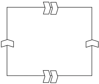
Network topologies explored here include geometric structures, namely the rectangle, cylinder,

torus, mobius strip, and Klein bottle, and all of which may be decomposed to a rectangle. The

diagrams below demonstrate these structures and how they may be formed from the rectangle,

with like arrows depicting edge connections and the direction of the connection.

Fig. 3 Rectangle: No edges connected

13 Fig. 5a Torus: Opposite edges connected

Fig. 4 c Cylinder visualization [32]

Fig. 5b Torus visualization [33]

14

Fig. 7c Klein bottle visualization [35]

Fig. 7 a, b Klein bottle: Opposite points connected along one edge pair and like points connected along the other edge pair

15

5. IMPLEMENTATION

In this thesis the Kohonen Self Organizing Map algorithm is implemented as described in section

3.3. Also implemented are different network topologies for the SOM as discussed in Section 4.

Implementation of different topologies involved changes to the neighborhood function used to

indicate which nodes should be updated along with the best matching unit. Since these geometric

configurations could all be constructed from a rectangle, this meant creating some form of

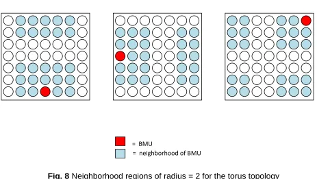
continuity along rectangle edges, with variations for the different shapes. For example, in the

torus vertical edges could be considered as being continuous, likewise for horizontal edges. In

this way the neighborhood regions could extend across rectangle boundaries wrapping around to

the opposite side of the rectangle as pictured below:

A range of experiments were carried out analyzing the map‟s clustering performance, varying

aspects such as the type of input data (randomly generated, 1 dimensional binary, high contrast

patches, face images and natural scenes), map cortex size spanning a range 15 x 15 to 60 x 60,

Fig. 8 Neighborhood regions of radius = 2 for the torus topology

= BMU

16

and different network topologies, including the rectangle, cylinder, torus, mobius strip, and Klein

bottle.

All implementations, training and testing were done in Matlab in order to make use of the

capabilities provided in their image processing tool kit.

6. DATA

Datasets used in training and testing include, The Cohn-Kanade Facial Expressions Database

[11], and the AT&T Database of faces (formerly the ORL Database of Faces) [1], the

Figure-Ground Dataset of Natural Images [3], and the Oliva and Torralba Dataset of Urban and Natural

Scene Categories [22]. Data also includes randomly generated values from different

distributions, 1-dimensional images, high contrast data patches as well as some web-gathered

images. All image processing is done on grayscale or binary data.

7. EXPERIMENTS AND RESULTS

The aim of these experiments is to investigate the clustering ability of the self organizing map

particularly on different types of data, with different cortex sizes and having different network

topologies.

The SOM trained for data clustering can typically be tested for its ability to class a new input

data, not previously seen in training into one of regions of the SOM. Given a data vector a

maximum response node of the SOM can easily be found by apply Euclidean distance

calculations as done in training to determine the best matching unit. The weights at the nodes of

the SOM can be reshaped to the original dimensions of an instance of the input data in order to

visualize and compare the appearances of nodes.

Kiviluoto [14], also describes bases for quantifying the „goodness‟ of a trained SOM. These are

17

well the map reflects probability distribution in the input space [14]. The latter Kiviluoto

explains is general accomplished well enough in the SOM, and therefore focuses on the aspects

of continuity and resolution. He defines continuity as being characterized by input vectors which

are close in input space being mapped closely in output space, while a mapping having a good

resolution he describes as one in which distant vectors of the input space will not be mapped

closely. Kiviluoto explains that a desirable factor for high resolution is “automatic selection of

feature dimensions” which occurs when the SOM output dimensions are lower than the

dimensions of the input manifold and the SOM attempts to approximate the higher dimensions

by folding itself like a Peano-curve. This approximation, though desirable for good resolution

compromises the continuity of the map. Resolution of the map can be measured via quantization

error Ԑp where the average distance from a set of sample vectors x to their best matching weight

vectors w is taken. Kiviluoto defines a measure for continuity as the topographic error Ԑt [14],

which sums local discontinuities throughout the SOM. Given a set of samples x, it is assumed

that its best matching weight vector wi and second best matching weigh vector wj will be

adjacent in an ideally continuous map. If this is not the case then there is a local discontinuity.

Discontinuity throughout the map is obtained by summing local discontinuities and normalizing.

Topographic error Ԑt is calculated by the following equation:

It is expected that for a given set of training data the self organizing map will provide a two

dimensional visualization of the data in which regions that are most like each other will be

arranged closest while most unlike regions will be furthest apart. Therefore distinctive clusters

should be observed in map. Since the SOM also has the property of topological preservation, we

additionally expect that the elements of these clusters formed will have a very similar if not

18

observe clusters of different textures throughout the map. We should further notice, that at

regions where clusters change, there should be smooth transitions with overlapping features of

adjacent clusters as the neighborhood radius decreases gradually, so the regions around cluster

perimeters are not dominated by any particular data instances.

With regard to the network topology our expectations are that more complex configurations of

the SOM will yield better clustering performance. As the model deviates from the rectangle, we

find that clusters forming around the perimeter of the rectangle are allowed to expand as they

become less bounded by abrupt edges. Allowing for more continuity therefore should allow for

more observable features in the map, and more graceful transitions.

In each of the sessions described below SOMs were trained on cortex sizes of 15 x 15, 30 x 30,

and 60 x 60 and for all topological models mentioned, and with a learning rate of 0.04.

Additional training on cortex sizes of 7 x 7, 22 x 22 and 45 x 45 has also been done for facial

expressions data.

7.1 Randomly Generated Data

This session of training involved using random data generated from a number of different

distributions including: uniform distribution, Gaussian distribution, binomial distribution,

exponential distribution, geometric distribution and Poisson distribution. Each training set

consisted of 500 data instances, each a 2x2 patch taken from the distributions. Training was done

for 50 epochs. Some of the results of training on randomly generated data are as follows:

19

Data including 100 observations from each distribution was then trained on a single SOM with

the following result for the triangle-topology SOM:

Tests were then done taking 500 observations, not included used in training, from each

distribution and displaying their corresponding maximum response nodes on the SOM. These

results are shown below; maximum response nodes are highlighted in black for each distribution:

Fig. 10 Rectangle-topology SOM (60 x 60 cortex) trained on data collectively from binomial, uniform, exponential, Gaussian, geometric and Poisson distributions

Fig. 11 Rectangle-topology SOMs (60 x 60 cortex) displaying maximum response nodes of 500 observations of binomial, uniform, exponential, Gaussian, geometric and

20

7.2 One Dimensional Images

Training on one dimensional data involved using two types of binary data vectors. The first set

consisted of data vectors having a single fixed length block of 1s with all other values 0. This

block of 1s was rotated to each position in the vector, with and without a wrap around. The

second set was constructed similarly to the first but consisted of 2 fixed length blocks of ones. In

this set the size of the block of 0s coming between the 2 blocks of 1s was varied between the two

extremes of having both blocks occurring with a maximum distance, to having them merge into a

single block. 1x25 data vectors were used for both types of data.

Type A Example: 0000000000111110000000000

 0000000000011111000000000

 0000000000001111100000000

Type B Example 1: 0000011111000001111100000

 0000001111100000111110000

 0000000111110000011111000

Type B Example 2: 0000001111110011111100000

 0000001111110111111000000

 0000001111111111110000000

21

7.3 High contrast patches

Gathering of high contrast data involved a method described by Mumford, Lee and Pedersen

[20]. 5000 random 3 x 3 intensity patches were chosen from each of 100 images from the Figure

Ground Dataset of Natural Images [3]. Of these patches the top 20% having the highest contrast

Fig. 12 Cylinder-topology SOMs (60 x 60 cortex) for non-wrapped and wrapped A-type data respectively. Length of block of 1s = 5

Fig. 13 Cylinder-topology SOMs (60 x 60 cortex) for non-wrapped and wrapped B-type data respectively. Length of block of 1s = 5

22

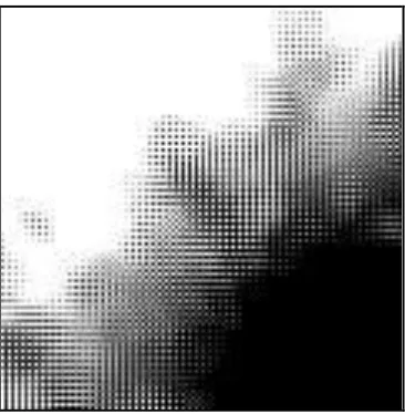
were retained. The SOM was trained on 200 of these patches, for 200 epochs, giving the

following results:

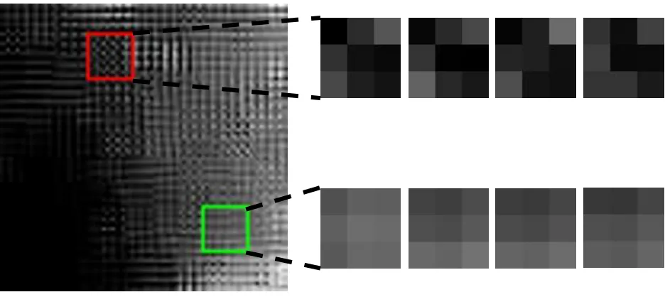
Two regions of the rectangular SOM were then select and 4 random patches from each region

inspected as shown below:

Fig. 15 Results of training the SOM on 3 x 3 high contrast patches. Showing topologies in order of appearance: rectangle, cylinder, torus, mobius strip, Klein bottle

(30 x 30 cortex size)

23

7.4 Natural/Outdoor Scenes

The SOM was also trained on images of natural and outdoor scenes. Data used for training and

testing included web-gathered images as well as images from the Oliva and Torralba dataset of

Urban and Natural Scene Categories [22]. Training data consisted mostly of images of natural

and outdoor scenes; buildings and trees/vegetation. Data processing involved dividing images of

higher dimensions into smaller sized patches, such as 25 x 25 and 8 x 8, and using each patch as

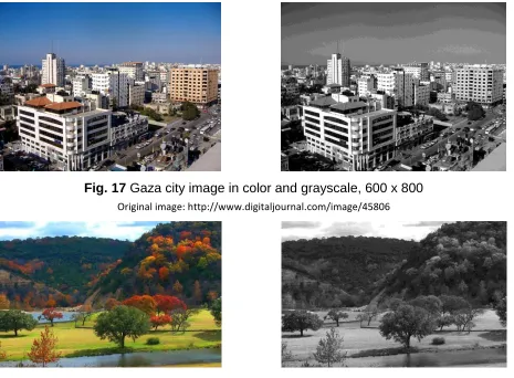
an individual data instance. The following images split up into 25 x 25 patches and used in

training:

Fig. 17 Gaza city image in color and grayscale, 600 x 800

Fig. 18 Texas Hill Country image in color and grayscale, 600 x 800

Original image: http://www.digitaljournal.com/image/45806

24

The sets of 25x25 patches for these images were each trained separately then with combinations,

for 50 epochs. Some of the results are as follows:

Fig. 20 Building image in color and grayscale, 175 x 275 Fig. 19 Apple tree image in color and grayscale, 200 x 250

25

Fig. 21 Results of training 25x25 patches from Gaza Image on 15x15 Cylinder SOM

26

Fig. 23 Results of training 25x25 patches from Texas Image on 60x60 Torus SOM

27

Additional training on natural and outdoor images involved use of images from the Oliva and

Torralba Dataset [22]. This database consists of outdoor images spanning eight categories of

urban and natural scenes. These categories include coast and beach, open country, forest,

mountain, highway, street, city center and tall building. One image from each category was

selected for training. The training images were converted to grayscale, resized from 256x256 to

128x128, and split up into 8x8 patches. Patches having no contrast were then discarded. The

following images were used in training:

coast forest highway city

28

mountain open country street tall building

The following is an example of the system having train on these images with a 60x60 cortex size

and Klein bottle topology:

Fig. 26 Urban and natural scene images used in training (original images from Oliva and Torralba dataset [22])

29

A process of false coloring was then applied to the training images to determine what regions of

the SOM patches from that image were clustered into. The process of false coloring involved

dividing the SOM into four equally sized quadrants each of which was assigned one of four

colors: red, green, blue and white. Maximum response nodes for each 8x8 training patch was

found on the SOM, and based on the region of the SOM which that patch fell into the training

image was assigned its corresponding color. Division of SOM into quadrants was done according

to topology as shown below, where regions of the same color are a part of the same quadrant:

Rectangle Cylinder

Torus Mobius Strip

R

G

K

B

R

G

K

B

R

B

R

G

K

B

R

B

R

G

K

B

R

B

30

Klein Bottle

Fig. 28 Guide for false coloring in different topologies

R

G

K

B

R

B

R

G

R

31

The resulting false colored training images are as displayed below. It must be noted that due to

randomness of initialization the same clusters may fall in different quadrants for different SOMs

but the relationship between and within clusters should be preserved. The results displayed relate

to the 60x60 SOM configured as a Klein bottle. All training images have been false colored

based on the same SOM (fig.).

coast

32

forest

highway

city

33

open country

street

tall building

Eight testing images were selected, also from the Oliva and Torralba dataset [22], one image

from each category, converted to grayscale and resized to 128x128. The selected training images

are displayed below. Some of these images, although falling under distinct categories in the

dataset, also possessed some features from other categories, for example the coast, tall building

34

and highway images also included vegetation, the open country also included mountainous areas,

etc. The test here was intended to show some aspect of consistency in texture within images from

the same category.

coast forest highway city

mountain open country street tall building

coast

35

forest

highway

city

36

open country

street

tall building

7.5 Face Images

The system was also trained on face images from the AT&T Database of Faces [1]. Initially the

following four faces were chosen:

37

These images were cropped to just the face portion and resized to 25 x 25. Face images will

hereafter be referred to Subject 1, Subject 2, Subject 3 and Subject 4, in order of appearance in

the above figure. The SOM was trained on a single image of each of these four subjects for 1000

epochs, with the network configured in each of the topologies previously mentioned. Below are

some results of training on an SOM having a 15 x 15 cortex size:

Fig. 34 25x25 face images used for training [~#1]

38

Cylinder (b) Torus

39

Training on face images was extended to incorporate a variety of facial expressions and poses.

These tests were done to further show the topology preserving property of the self organizing

map. Data included faces with happy, sad, surprised and neutral expressions as well as right and

left face profiles. Images used in training and testing were taken from the AT&T database of

faces [1], the Georgia Tech face database [6], and the Cohn-Kanade AU Coded Facial

Expressions Database [11]. For training multiple instances of each type of expression/pose was

used, with each image being taken from a different subject. Since faces were taken from different

databases all images were converted to grayscale, cropped to 25x25 and normalized to

zero-mean and unit variance in an attempt to eliminate learning of lighting variations over facial

expressions. Normalization was done within each image as well across the entire training set.

The following are examples of the images used in training:

Klein Bottle (a) Klein Bottle (b)

40

The expectation for this experiment was that similar expressions and poses would cluster in

roughly the same region. Training was performed on 6 cortex sizes, including: 7x7, 15x15,

22x22, 30x30, 45x45 and 60x60. A resulting 22x22 SOM is shown below:

Fig. 36 Face images used for training SOM on facial expressions and poses. ([~#1], [6], [11])

41

Tests were also done using faces not seen in training, and finding the max response nodes for

these images. These tests included, in some instances, using multiple images of a single

individual having different facial expressions and observing if these images would be mapped to

nodes close together, or to clusters having a similar facial expression or pose. The following

images were used for testing:

Some results of test faces compared with their maximum response nodes are shown below. Each

set of images represents a portion of the results from a SOM trained with a different cortex size.

7x7

15x15

22x22

30x30

42

45x45

60x60

The following diagram shows the positions on the SOM of figure 37 of the maximum response nodes for same individuals (subjects A, B, C) having different facial expressions:

Fig. 39 Test images (left) along with their max response nodes (right)

C-surprised, (9, 22)

C-happy, (11, 4) B-left profile, (19, 21) B-right profile, (16, 17) A-happy, (11,6) A-sad, (12,19)

43

Tests were also done on the following non-face images which resulted in the corresponding maximum response nodes as shown:

Other investigations done in these tests involved inspection of distances of new images from max

response nodes and how they can be compared for different cortex sizes of the SOM as well as

different topologies. These results were recorded to determine what effects if any these aspects

might have on the clustering ability of the SOM and why. Experiments on facial expressions

were also used to determine the quality of the SOM according to Kiviluoto‟s goodness criteria.

Statistics are summarized as follows:

44

Mean Distances For Test Face Images

Rectangle Cylinder Mobius

Strip

Torus Klein MEAN

7x7 _{2.8032 2.7651 2.8148 2.8110 2.7720 2.7932}

15 x 15 _{2.7839 2.7918 2.7717 2.7754 2.7711 2.7788}

22 x 22 _{2.8106 2.7980 2.7799 2.7698 2.7583 2.7833}

30 x 30 _{2.8201 2.7930 2.7725 2.7688 2.7893 2.7887}

45 x 45 _{2.7829 2.7919 2.7908 2.7697 2.7642 2.7799}

60 x 60 _{2.7938 2.7931 2.7720 2.7596 2.7347 2.7706}

MEAN _{2.7991 2.7888 2.7836 2.7757 2.7649}

Mean Distances For Test Non-Face Images

Rectangle Cylinder Mobius

Strip

Torus Klein MEAN

7x7 _{4.1716 4.1617 4.2056 4.1095 4.1461 4.1589}

15 x 15 _{4.2345 4.2705 4.2975 4.1939 4.2181 4.2429}

22 x 22 _{4.3181 4.1795 4.2008 4.1965 4.2088 4.2207}

30 x 30 _{4.2395 4.2343 4.2822 4.2201 4.1354 4.2223}

45 x 45 _{4.2803 4.2603 4.2490 4.1270 4.2199 4.2273}

60 x 60 _{4.2661 4.2328 4.2327 4.2140 4.1241 4.2139}

MEAN _{4.2517 4.2232 4.2446 4.1768 4.1754}

Table 1. Comparison of means distances from maximum response nodes by cortex size and topology (test faces)

45

SOM Continuity

Adjacency of best and 2nd best matching nodes by cortex size

7 x 7 15 x 15 22 x 22 30 x 30 45 x 45 60 x 60

Face 1 _{0 1 0 1 1 0}

Face 2 _{0 1 0 0 0 0}

Face 3 _{1 1 1 1 1 1}

Face 4 _{0 1 0 0 0 0}

Face 5 _{0 0 0 0 0 0}

Face 6 _{0 1 0 0 1 0}

Face 7 _{0 1 1 1 0 1}

Face 8 _{0 0 0 0 0 1}

Face 9 _{0 1 0 1 1 0}

Face 10 _{0 0 0 1 1 0}

Face 11 _{0 0 0 0 0 1}

Face 12 _{0 0 0 0 0 1}

Face 13 _{0 0 0 1 1 1}

Face 14 0 0 0 1 0 0

Face 15 1 0 0 1 0 1

Face 16 0 1 0 0 1 1

Face 17 0 0 0 0 1 1

Face 18 0 0 0 1 0 0

Face 19 0 0 0 0 0 0

Face 20 0 0 1 1 1 0

Face 21 0 1 0 0 0 1

Face 22 0 0 1 0 1 1

Face 23 0 0 0 0 0 0

Face 24 0 1 0 1 0 1

Face 25 1 0 0 1 1 1

Face 26 0 0 0 0 1 0

SUM: 3 10 4 12 12 13

Top Error 0.115385 0.384615 0.153846 0.461538 0.461538 0.5

46

8. ANALYSIS

Here we examine the results of the SOMs produced above, analyzing stricture and clusters

formed, as well as evaluate the SOM on its ability to assign data not seen in training to the

cluster region of the map most like itself as well as analyze them based on Kiviluoto‟s goodness

criteria [14] and determine the effect that the network topology may have had on the final

product.

8.1 Random Data

The experiments done on random data from varying distributions can be seen to demonstrate the

maps capability to adequately cluster similar observations of data. Based on the appearance of

the data of individual distributions compared with the SOM having all distributions combined,

along with the evidence of the regions of max response for each distribution, we can observe that

instances from the binomial distribution, having most values equal to or very close to 1, being

clustered at the top, merging into observations from the geometric distribution, which are

sparsely populated with some light gray level values, and so on until arriving at a cluster of the

data from the Poisson distribution at the bottom, having mostly values of or very close to 0.

The clusters therefore smoothly transition from lightest to darkest intensity values, from top left

to bottom right of the SOM, thereby allowing us to see which distributions are more closely

related to or dissimilar from others. We may even extend this to gain more insight into aspects

such as relative parameters values of functions used in obtaining a set of data values as well as

how wide or narrow a range one set of data might Hence we see that having no prior knowledge

of a set of data values we can use such a system for classification of instances of this data into

their most probable distribution.

8.2 One-Dimensional Images

We may visualize the nodes of the SOMs formed in this experiment as having a single row of 25

47

these experiments in that we are able to see the distinct and in most areas non-overlapping

patterns made by the fixed blocks of 1s (white regions of the SOM). These patterns arise due to

the small incremental shifts in the blocks of 1s, with each instance of data. So for each node of

the SOM adjacent nodes (nodes within a neighborhood of radius = 1) would have a shift of

approximately 1 pixel in the block of 1s, nodes within a neighborhood of radius=2 would have a

shift of approximately 2 in the block of ones, and so on.

We further see structure maintained in the B-type data (figure 14) where the block of zeros

between the blocks of 1s is varied from its initial width to 0, as well as overlapping of the blocks

ones. Here we see that the patterns of the SOM grid consist mostly of convergence and

divergence of sets of light pixels, representative of decreases (convergence) and increases

(divergence) in the distances between the blocks of 1s.

We can also perceive the structures of the mobius strip and Klein bottle topologies in figures 13

and 14 where patterns at opposite ends of the SOMS appear equivalent but inverted. This

structure confirms that these regions are considered to be adjacent in these topologies.

8.3 High Contrast Patches

Identical transitional patterns as previously described can also be observed in the clustering of

high contrast data experiment. We can additionally visualize with actual data, how each different

topological models of the SOM will cluster the same data set. We notice a greater variation in the

arrangement of the clusters as the network configurations vary among the different topologies.

The rectangular topology, being confined on each edge restricts growth of clusters and shows

abrupt cluster ends at edges. As a greater degree connectivity is introduced in successive

topologies we can see continuity of regions on the right to left edges of the cylinder, right to left

and top to bottom of the torus, top left to bottom right of the mobius strip and vice versa, and

48

Closer inspection of 3 x 3 patches reveals a similarity in structure of patches from neighboring

regions. These patches are almost consistent in the variety of pixel intensity values contained

within them. In Figure 16, patches of the red bounded region can be characterized as having high

contrast in relation to the lower contrast patches of the green bounded region and are therefore at

opposite ends of the rectangular topology SOM.

8.4 Natural Images and Outdoor Scenes

Again, in training web gathered images, we can see identifiable patterns in clustered regions of

the resulting SOMS and smooth transitions between clusters. Training on small patches of

natural images allowed for clustering of low level features of image texture.

The false coloring of images from the Oliva and Torralba dataset [22] enables us to better

understand relationships between textures in different regions of the images. Thus, regions which

have been colored identically can be ideally thought of to have closest texture to each other and

be more dissimilar to regions having a different color.

In the training dataset we can therefore make some associations between textures of the buildings

of the city image, the beach and sky in the coast image as well as the mountain image which

have all been predominantly colored with red. The texture of the open country is however some

measure of distance away with regard to texture, having been mostly colored in black, while the

highway image having more activity in the scene by way of different objects or segments with

different textures, has an approximately equal mixture of colors spanning each quadrant of the

SOM.

Examining the close ups of the nodes in different regions of the SOM we see that patches in the

red region consist mostly of pixels of darker intensity and very few lighter pixels, patches in the

black region consist of sharp contrasts with dark bands along edge pixels, and lower contrast

within the rest of the patch, patches in the blue region consist of roughly intermediate gray-level

49

consist of light gray-level values with a darker number of pixels in the bottom right corner,

possibly characteristic of edges of objects in the image.

Some of the training images for example forest and mountain were for the most part consistent in

the predominant color of the training image from the same category, others such as city and

highway were not as representative of the training images. This may have been due to general

differences of scene content, angle of the photo, and lighting conditions within scene categories.

It is however worth noting that the system performed quite adequately in segmentation within

individual images as the scene transitioned from sky to building/mountain/highway and between

different objects of the scene.

The false coloring process could also be enhance by having more regions of color as in images

such as natural scenes there can be many different textures and potential for numerous clusters.

A four color limit would therefore may not accurately representative of the intra-regional

distinction of textures, particularly on SOMs having a large cortex.

8.5 Face Images

The network topology is also well demonstrated in the images of Figure 35 showing clusters of

four faces. As the network structure moves away from the rectangle we are more able to

visualize wrap-around regions as seen in the torus SOM, for example, where clusters of Subjects

1 and 3 can be seen wrapping around the horizontal edges of the map, Subject 2 wrapping around

the vertical edges, and subject 4 clustering toward the middle. Regions where clusters meet can

also be seen in transition with faces having features overlapping adjacent clusters.

The system also performs commendably at clustering similar facial expressions. In the SOM of

Figure 37, faces showing a left profile can be seen clustered at the bottom right and wrapping

around to the top right, faces with a right profile can be seen clustered at the bottom middle and

extending upwards, merging into smiling faces with a right profile and then frontal smiling faces

50

expressions can be found at the right and left edges toward the middle, merging into frowning

faces on the left.

Results for test faces compared with their maximum response nodes show for the most part that

the SOM does a good job in categorizing a newly seen face with nodes displaying its expression,

with the exception of just a few. It can also be notices that faces of the same individual are

categorized with like expression/pose clusters.

8.6 Quantifying Goodness

Experiments on facial expression data were also used in determining goodness of the SOM as

described by Kiviluoto [14] with regard to resolution and continuity.

With the SOM folding itself in an attempt to approximate higher dimensions, for lattice

dimensions smaller than training data manifold dimensions, the resolution of the map should be

enhanced. The data of Table 1 does not reflect any recognizable pattern in quantization errors

with increases of cortex size, a much larger test set may make these results more definable. We

can, however, glean from this table that topology does in fact play a part in SOM performance as

we see that as connectivity increases from rectangle to Klein Bottle there is a steady decrease in

quantization error .

With regard to continuity, it can be seen from table 3 that the 7x7 cortex gives the lowest

topographic error, while the 60x60 cortex gives the highest error. The data shows maps of larger

cortex sizes generally having a greater topographic error, hence being less continuous.

We also make note of the behavior of the SOM when classifying non-face images. The distances

of non-faces from their maximum response nodes are considerably higher than those of faces,

having values over 4 while distances of faces from their best match lie within the range 2-3. We

can therefore use the SOM to detect inconsistencies of test data with training data. This would

51

9. CONCLUSION

To conclude, we have ascertained that the Kohonen Self Organizing Map network is one in

which adequate and efficient data clustering can be performed. Not only this, but the

self-organizing map also possesses the property of topological preservation of training data.

Through a number of experiments we have shown the ability of the map to make natural

associations particularly between regions of images and general image content.

We have also explored how we may determine goodness of a SOM with measures of its

resolution and its continuity.

We have further seen that the map may be configured in a number of different models, including

those attempted in these experiments: the rectangle, cylinder, torus, mobius strip, and Klein

bottle. We may deduce that with connectivity being introduced into the map these models are

52

10. REFERENCES

[1] AT&T Laboratories Cambridge, “The AT&T Database of Faces”, [~#Online]. Available:

http://www.cl.cam.ac.uk/Research/DTG/attarchive/pub/data/att_faces.zip

[2] L. Fausett, “Fundamentals of Neural Networks: Architectures, Algorithms and Applications”, Prentice-Hall, Englewood Cliffs, NJ, 1994

[3] C. Fowlkes, D. Martin, J. Malik. "Local Figure/Ground Cues are Valid for Natural Images" Journal of Vision, 7(8):2, pp. 1-9, [~#Online]. Available:

http://journalofvision.org/7/8/2/Fowlkes-2007-jov-7-8-2.pdf

[4] G. Fung. A Comprehensive Overview of Basic Clustering Algorithms, June 22, 2001, [~#Online]. Available:

http://citeseerx.ist.psu.edu/viewdoc/download?doi=10.1.1.81.5037&rep=rep1&type=pdf

[5] B. Gao, T. Liu, T. Qin, X. Zheng, Q. Cheng, W. Ma, “Web image clustering by consistent utilization of visual features and surrounding text”, in Multimedia '05:

Proceedings of the 13th annual ACM international conference on Multimedia (2005), pp.

112-121.

[6] Georgia Tech Face Database, [~#Online]. Available:

http://www.anefian.com/research/gt_db.zip

[7] R. Ghrist, “Barcodes: The Persistent Topology of Data”, in Bulletin of the American

Mathematical Society, Vol. 45, No. 1, 2008, pp. 61-75.

[8] J. H. van Hateren and A. van der Schaaf, “Independent Component Filters of Natural Images Compared With Simple Cells in Primary Visual Cortex”, in Proceedings: Biological Sciences, Vol. 265, No. 1394, March 1998, pp. 359-366.

[9] P. Jeyanthi and V. Jawahar Senthil Kumar, “Image Classification by K-Means”, in

Advances in Computational Sciences and Technology, ISSN 0973=6107, Vol. 2, No. 1,

2010, pp. 1-8.

53

[11] T. Kanade, J. F. Cohn and Y. Tian, (2000) “Comprehensive Database for Facial Expression Analysis”, in Proceedings of the Fourth IEEE International Conference on

Automatic Face and Gesture Recognition (FG’00), Grenoble, France, pp. 46-53.

[12] J. Kangas and T. Kohonen, “Development and Applications of the Self-Organizing Map and Related Algorithms”, in Mathematics and Computers in Simulation, Vol. 41, July 1996, pp. 3-12.

[13] C. Kemp and J. B. Tenenbaum, „The discovery of structural form‟, In Proceedings of the

National Academy of Sciences of the United States of America, Department of

Psychology, Carnegie Mellon University, 5000 Forbes Avenue, Pittsburgh, PA, July (2008)

[14] K. Kiviluoto, “Topology preservation in self-organizing maps”, in IEEE International

Conference on Neural Networks, vol. 1, June 1996, pp. 294-299.

[15] T. Kohonen, “The Self Organizing Map”, in Proceedings of the IEEE, Vol. 78, No. 9. (06 Sept 1990), pp. 1464-1480

[16] T. Kohonen, O. Simula and J. Kangas, “Engineering Applications of the Self-Organizing Map”, in Proceedings of the IEEE, vol 84, No. 10, October 1996, pp. 1358-1384.

[17] S. Krishnamachari and M. Abdel-Mottaleb , “Hierarchical Clustering Algorithm for fast Image Retrieval”, in IS&T/SPIE Conference on Storage and Retrieval for Image and

Video databases VII, 1999, pp. 427-435

[18] S. Krishnamachari and M. Abdel-Mottaleb, “Image browsing using hierarchical clustering," in Proceedings of the fourth IEEE International Symposium on computer and

communications, Egypt, July 1999.

[19] A Martinez, P. Mittrapiyanuruk and A. C. Kak, “On combining graph-partitioning with non parametric clustering for image segmentation”, in Computer Vision and Image

Understanding Vol. 95, 2004, pp. 72-85.

[20] D. Mumford, A. Lee, and K. Pedersen, “The nonlinear statistics of high-contrast patches in natural images,” Intl. J. Computer Vision, Vol. 54 (2003), 83–103.

54

International Journal of Engineering Science and Technology Vol. 2(3), 2010, pp.

209-212.

[22] A.Oliva and A. Torralba “Modeling the Shape of the Scene: A Holistic Representation of the Spatial Envelope”, International Journal of Computer Vision, 2001, Vol. 42, No. 3, pp. 145-175.

[23] J. Philbin, O. Chum, M. Isard, J. Sivic, and A. Zisserman. “Lost in Quantization: Improving Particular Object Retrieval in Large Scale Image Databases”, Proceedings of

the IEEE Conference on Computer Vision and Pattern Recognition, 2008.

[24] J. Philbin, O. Chum, M. Isard, J. Sivic, and A. Zisserman. “Object retrieval with large vocabularies and fast spatial matching”, Proceedings of the IEEE Conference on

Computer Vision and Pattern Recognition, 2007.

[25] G. Qiu, “Bipartite graph partitioning and content-based image clustering”, in 1st

European Conference on Visual Media Production, March 2004, pp. 87-04.

[26] K.S. Ravichandran and B. Ananthi, “Color Skin Segmentation Using K-Means Cluster”,

in International Journal of Computational and Applied Mathematics, ISSN 1819-4966,

Vol. 4, No. 2, 2009, pp. 153-157.

[27] M. Turk and A. Pentland, "Eigenfaces for recognition," Journal of Cognitive

Neuroscience, vol. 3, no. 1, pp. 71-86, January 1991.

[28] [~#Online]. Available: http://en.wikipedia.org/wiki/Cluster_analysis

[29] [~#Online], Available: http://en.wikipedia.org/wiki/Graph_partitioning

[30] [~#Online]. Available: http://en.wikipedia.org/wiki/Self-organizing_map

[31] [~#Online]. Available: http://www.ai-junkie.com/ann/som/som1.html

[32] [~#Online]. Available: http://etc.usf.edu/clipart/41700/41702/fc_cylinder_41702.htm

[33] [~#Online].Available:

http://www.math.cornell.edu/~mec/2008-2009/HoHonLeung/page6_knots.htm

[34] [~#Online]. Available: http://local.wasp.uwa.edu.au/~pbourke/geometry/mobius/