Computation of Laminated Composite Plates using Integrated Radial Basis
Function Networks
N. Mai-Duy1, A. Khennane2 and T. Tran-Cong3
Abstract: This paper reports a meshless method, which is based on radial-basis-function networks (RBFNs), for the static analysis of moderately-thick laminated composite plates us-ing the first-order shear deformation theory. Inte-grated RBFNs are employed to represent the field variables, and the governing equations are dis-cretized by means of point collocation. The use of integration rather than conventional differen-tiation to construct the RBF approximations sig-nificantly stabilizes the solution and enhances the quality of approximation. The proposed method is verified through the solution of rectangular and non-rectangular composite plates. Numerical re-sults obtained show that the method achieves a very high degree of accuracy and a fast conver-gence rate.
Keyword: laminated composite plate, radial-basis-function network, meshless method.
1 Introduction
Principal discretization methods for solving par-tial differenpar-tial equations (PDEs) include a finite-difference (FD), finite-element (FE), boundary-element (BE), finite-volume (FV) and spectral method. Among them, the FEM is the most widely used method in computational engineer-ing. To integrate a weak form and interpolate a solution variable, the FEM requires the division of the domain of interest into a number of small elements that are connected together by a fixed topology (i.e. mesh). This task is seen to be
1Computational Engineering and Science Research Centre,
USQ, Toowoomba, QLD 4350 Australia
2Computational Engineering and Science Research Centre,
USQ, Toowoomba, QLD 4350 Australia
3Computational Engineering and Science Research Centre,
USQ, Toowoomba, QLD 4350 Australia.
quite cumbersome especially for problems involv-ing complex geometries, large degrees of defor-mation and free/moving surfaces. The idea of de-veloping numerical methods without using a mesh for the solution of PDEs has received consider-able attention from the scientific and engineering research communities in recent decades. As the name suggests, there will not be any connectivity requirements between interpolation points, lead-ing to an easy process of numerical modelllead-ing. A comprehensive review of meshless methods can be found in, for example, [Atluri and Shen (2002);Liu (2003)].
approxi-64 Copyrightc 2007 Tech Science Press CMC, vol.5, no.1, pp.63-77, 2007
mation. As an alternative to the conventional di-rect/differentiated RBFN (DRBFN) method, Mai-Duy and Tran-Cong (2003), and Mai-Mai-Duy and Tran-Cong (2001) proposed the use of integra-tion to construct the RBFN expressions (the in-direct/integrated RBFN (IRBFN) method) for the approximation of a function and its derivatives and for the solution of PDEs. Numerical results showed that the IRBFN method achieves superior accuracy [Mai-Duy and Tanner (2005);Mai-Duy and Tran-Cong (2005);Mai-Duy and Tran-Cong (2006)]. The improvement is attributable to the fact that integration is a smoothing operation and is more numerically stable.
In this paper, the meshless IRBFN-based method is further developed for the static analysis of moderately-thick laminated composite plates us-ing the first-order shear deformation theory. The obtained results are compared to existing results from different methods reported in the litera-ture. Indeed, laminated fibre composite plates are extensively used in aeronautics and space industries, and much research effort has been dedicated to improve the ability to predict the behaviour of these structures. Closed form solutions based either on the first- or higher-order shear deformation theory (e.g. [Whitney and Pagano (1970);Bert and Chen (1978);Reddy and Chao (1981);Reddy (1984);Pandya and Kant (1988); Liu, Zhang, and Zhang (1994)]) as well as 3D elasticity solutions (e.g. [Srinivas and Rao (1970);Pagano and Hatfield (1972);Wang and Tarn (1994)]) are available to assess the accuracy of the numerical methods.
A brief review of the first-order shear deformation theory is given in Section 2. The governing equa-tions involve a large number of derivative terms, some of which are mixed partial derivatives. The discretization of these equations using DRBFNs and IRBFNs is presented in section 3. In section 4, the IRBFN method is used to analyze compos-ite plates with different geometries and boundary conditions. The obtained results show that the present method attains fast convergence rates and high degrees of accuracy. Section 5 gives some concluding remarks.
2 First-Order Shear Deformation Theory of Laminated Composite Plates
The first-order shear deformation theory (FSDT) of laminated composite plates is an extension of the Reissner-Mindlin theory for homogeneous isotropic thick plates. The governing differential equations are well known, and their derivation can be found in details in Reddy (2004). However, for the sake of consistency an outline of the main equations will be given below.
In FSDT, the displacement field is given as
u = u0+zψx, (1)
v = v0+zψy, (2)
w = w0, (3)
where(u0,v0,w0)are the displacements of a point
situated in the middle plane, thexyplane, andψx andψy are respectively the rotations of the trans-verse normal, i.e. in thezdirection, with respect to theyandxaxes.
In the present theory of thick plate without mem-brane action,u0andv0are discarded. As a result,
the strain displacement relationships are given as
εxx = −z∂ψx
∂x , (4)
εyy = −z∂ψy
∂y , (5)
γxy = z∂ψx
∂y −
∂ψy ∂x
, (6)
γyz = ∂w
∂y −ψy, (7)
γxz = ∂w
∂x +ψx. (8)
as
⎧ ⎪ ⎪ ⎪ ⎪ ⎨ ⎪ ⎪ ⎪ ⎪ ⎩
σxx σyy τxy τyz τxz
⎫ ⎪ ⎪ ⎪ ⎪ ⎬ ⎪ ⎪ ⎪ ⎪ ⎭
=
⎡ ⎢ ⎢ ⎢ ⎢ ⎣
Q11 Q12 Q16 0 0
Q12 Q22 Q26 0 0
Q16 Q26 Q66 0 0
0 0 0 C44 C45
0 0 0 C45 C55
⎤ ⎥ ⎥ ⎥ ⎥ ⎦
⎧ ⎪ ⎪ ⎪ ⎪ ⎨ ⎪ ⎪ ⎪ ⎪ ⎩
εxx εyy γxy γyz γxz
⎫ ⎪ ⎪ ⎪ ⎪ ⎬ ⎪ ⎪ ⎪ ⎪ ⎭
. (9)
The previous expression can be rewritten as
⎧ ⎨ ⎩
σxx σyy τxy
⎫ ⎬ ⎭=
⎡
⎣ QQ1121 QQ1222 QQ1626
Q16 Q26 Q66
⎤ ⎦
⎧ ⎨ ⎩
εxx εyy γxy
⎫ ⎬ ⎭ (10)
and
τyz τxz
=
C44 C45
C45 C55
γyz γxz
, (11)
where the termsQi jandCi jrepresent the stiffness
constants of a unidirectional orthotropic compos-ite making an angleθwith the principal material x-axis. They are given as
Q11 = Q11cos4θ+Q22sin4θ
+2(Q12+2Q66)sin2θcos2θ, (12)
Q12 = (Q11+Q22−4Q66)sin2θcos2θ +Q12(cos4θ+sin4θ), (13) Q16 = (Q11−Q12−2Q66)sinθcos3θ
+(Q12−Q22+2Q66)sin3θcosθ, (14)
Q22 = Q11sin4θ+Q22cos4θ
+2(Q12+2Q66)sin2θcos2θ, (15)
Q26 = (Q11−Q12−2Q66)sin3θcosθ
+(Q12−Q22+2Q66)sinθcos3θ, (16)
Q66 = (Q11+Q12−2(Q12+Q66)sin2θcos2θ +Q66(cos4θ+sin4θ), (17)
C44 = C44cos2θ+C55sin2θ, (18)
C45 = (C55−C44)cosθsinθ, (19)
C55 = C44sin2θ+C55cos2θ. (20)
The termsQi j andCi j represent the stiffness
con-stants of a unidirectional orthotropic ply in its
principal axes. They are given as
Q11 =
E1
1−ν12ν21,
(21)
Q22 =
E2
1−ν12ν21,
(22)
Q12 = ν12
E2
1−ν12ν21,
(23)
Q66 = G12, (24)
C44 = G23, (25)
C55 = G13. (26)
The moments and shears are defined as acting per unit length. They are given as
Mxx =
h/2
−h/2σxx
zdz, (27)
Myy =
h/2
−h/2σyy
zdz, (28)
Mxy =
h/2
−h/2τxy
zdz, (29)
Qx =
h/2
−h/2τxz
dz, (30)
Qy =
h/2
−h/2τyz
dz, (31)
where h is the thickness of the laminate. Sub-stituting for the stresses using equations (10) and (11), the moments and shear forces are rewritten as
⎧ ⎨ ⎩
Mxx
Myy
Mxy ⎫ ⎬ ⎭=
⎡
⎣ DD1112 DD1222 DD1626
D16 D26 D66
⎤ ⎦
⎧ ⎨ ⎩
εxx εyy γxy
⎫ ⎬ ⎭
(32)
and
Qy
Qx
=
A44 A45
A45 A55
γyz γxz
(33)
with
Di j=
1 3
n
∑
k=1(h3k−h3k−1)(Qi j)(k) i,j=1,2,6,
(34)
Ai j=κ n
∑
k=166 Copyrightc 2007 Tech Science Press CMC, vol.5, no.1, pp.63-77, 2007
whereκ=5/6 is a shear correction factor. Con-sidering the equilibrium of an infinitesimal plate element leads to the following equations
∂Qx ∂x +
∂Qy
∂y +q(x,y) =0, (36)
∂Mxy ∂x +
∂Myy
∂y =Qy, (37)
∂Mxy ∂x +
∂Mxx
∂x =Qx. (38)
Substituting for Qx , Qy, Mxx, Myy and Mxy, the
equilibrium equations become
A45 ∂2w
∂x∂y−
∂ψy ∂x
+A55 ∂2w
∂x2 + ∂ψx
∂x
+A44 ∂2w
∂y2 − ∂ψy
∂y
+A45 ∂2w
∂x∂y+
∂ψx ∂y
+q(x,y) =0,
(39)
D16
−∂2ψx
∂x2
+D26
−∂2ψy
∂x∂y
+D66 ∂2ψx
∂x∂y−
∂2ψy ∂x2
+D12
−∂2ψx
∂x∂y
+D22
−∂2ψy
∂y2
+D26 ∂2ψ
x ∂y2 −
∂2ψ y ∂x∂y
=A44 ∂w
∂y −ψy
+A45 ∂w
∂x +ψx
,
(40)
D16
−∂2ψx
∂x∂y
+D26
−∂2ψy
∂y2
+D66 ∂2ψx
∂y2 − ∂2ψy ∂x∂y
+D11
−∂2ψx
∂x2
+D12
−∂2ψy
∂y∂x
+D16 ∂2ψx
∂y∂x−
∂2ψy ∂x2
=A45 ∂w
∂y −ψy
+A55 ∂w
∂x +ψx
.
(41)
For a cross-ply laminated composite plate (00,900), the equilibrium equations reduce to
A55 ∂2w
∂x2 + ∂ψx
∂x
+A44 ∂2w
∂y2 − ∂ψy
∂y
+q(x,y)
=0, (42)
D66 ∂2ψx
∂x∂y−
∂2ψy ∂x2
+D12
−∂2ψx
∂x∂y
+D22
−∂2ψy
∂y2
=A44 ∂w
∂y −ψy
, (43)
D66 ∂2ψx
∂y2 − ∂2ψy ∂x∂y
+D11
−∂2ψx
∂x2
+D12
−∂2ψy
∂y∂x
=A55 ∂w
∂x +ψx
. (44)
3 Radial Basis Function Networks
RBFNs allow a conversion of a function from low-dimensional space (e.g., 1D-3D) to high-dimensional space in which the function can be expressed as a linear combination of RBFs [Haykin (1999)]
fe(x)≈ f(x) = m
∑
i=1w(i)g(i)(x), (45)
where fe and f are the exact and approximate
functions, respectively; superscripts denote the el-ements of a set of neurons;xthe input vector;m the number of RBFs;{w(i)}mi=1the set of network weights to be found; and {g(i)(x)}mi=1 the set of RBFs.
3.1 Direct (DRBFN) approach
The RBFN (45) is utilized to represent the orig-inal function fe; subsequently, its derivatives are
computed by differentiating (45), e.g. those with respect tox
∂fe(x) ∂x ≈
∂f(x) ∂x =
∂∑m
i=1w(i)g(i)(x)
∂x =
m
∑
i=1w(i)h(i)(x),
(46)
∂2f e(x) ∂x2 ≈ ∂2f(x)
∂x2 = ∂∑m
i=1w(i)h(i)(x)
∂x =
m
∑
i=1w(i)h(i)(x),
(47)
where h(i)(x) = ∂g(i)(x)/∂x and h(i)(x) = ∂h(i)(x)/∂x are new basis functions for the ap-proximation of the first- and the second-order derivatives of the original function fe,
3.2 Indirect (IRBFN) approach
RBFNs are used to represent the highest-order derivatives in the system under consideration, e.g., ∂2fe/∂x2 and ∂2fe/∂y2. Lower-order
derivatives and the function itself are then ob-tained by integrating those RBFNs, e.g. those with respect tox
∂2f e(x) ∂x2 ≈
∂2f(x) ∂x2 =
m
∑
i=1w([xi)]g(i)(x), (48)
∂fe(x) ∂x ≈
∂f(x) ∂x =
m+q1
∑
i=1w[(xi)]H[(xi])(x), (49)
fe(x) ≈ f[x](x) = m+q2
∑
i=1w[(xi)]H[(xi)](x), (50)
where subscript[x]denotes the quantities result-ing from the process of integration along the x direction; q1 the number of new centres in a
subnetwork that is employed to approximate a set of nodal integration “constants”, q2 =2q1;
and H[(xi]) = g(i)dx and H[(xi)] = H[(xi])dx (i = 1,2,···,m) new basis functions for the approxi-mation of the first-order derivative and the origi-nal function fe, respectively. For convenience of
presentation, the new centres and their associated known basis functions in subnetworks are also de-noted by the notationsw(i)andH(i)(x)(H(i)(x)), respectively, but withi>m.
There are two expressions, namely f[x](x) and f[y](x), to represent the function f(x)(
w[x]
=
w[y]
). At the collocation points, they are forced to be exactly the same, i.e., f[x](x) = f[y](x) =
f(x) (these nodal function values are unknowns to be found); at other points, the function fcan be taken to be the average value of f[x](x)and f[y](x). For 1D problems, the system matrices obtained by the DRBFN and IRBFN methods have similar sizes for a given number of data points; for 2D and 3D problems, the unknown vector of the latter is much larger than that of the former. To overcome this drawback, prior conversions of the multiple spaces of network weights into the single space of nodal variable values are necessary. The eval-uation of (48)–(50) at a set of collocation points
{x(k)}kp=1={c(k)}mk=1, withp=m, yields
f,xx = Gw[x], (51)
f,x = H[x]w[x], (52) f = H[x]w[x], (53)
where G, H and H are the design matrices as-sociated with the approximation of the second-order derivative, the first-second-order derivative and the function, respectively; w[x] is the set of
net-work weights in the x direction to be found;
f={f(x(k))}km=1; f,x={∂f(x (k))
∂x }mk=1; and f,xx=
{∂2f(x(k))
∂x2 }mk=1. For the purpose of computation, the two matrices Gand H are augmented using zero-submatrices so that they have the same size as the matrixH. By solving (53) with the general linear least-squares technique, the set of network weights can be expressed in terms of the nodal function values, as
w[x]=H− 1
[x]f, (54)
whereH−[x1] is the Moore-Penrose pseudo-inverse; and the dimensions of w[x], H−
1
[x] andf are(m+
q2)×1,(m+q2)×mandm×1, respectively.
Substituting (54) into the system (51)-(53) yields
f,xx = GH−
1
[x]f, (55)
f,x = H[x]H− 1
[x]f, (56)
f = If, (57)
where I is the unit matrix. Cross derivatives
∂f2(x)/∂x∂ycan be straightforwardly computed using the design matrices associated with the first-order derivatives (56). Although the first-order of dif-ferentiation makes no difference theoretically, due to numerical error, it would be more accurate to take the average of the two equivalent representa-tions,
∂2f ∂x∂y =
1 2
∂ ∂x
∂f
∂y
+ ∂
∂y
∂f
∂x
,
f,xy= 1 2
H[x]H−[x1]
H[y]H−[y]1f
+
H[y]H−[y]1
H[x]H−[x]1f
68 Copyrightc 2007 Tech Science Press CMC, vol.5, no.1, pp.63-77, 2007
Expressions of fand its derivatives at an arbitrary pointxcan be given by
f(x) =1
2
H[(x1])(x),···,H[(xm]+1)(x),···,
H(m+q1+1)
[x] (x),···H
−1
[x]f
+1 2
H[(y1])(x),···, H[(ym]+1)(x),···,
H(m+q1+1)
[y] (x),···
H−[y]1f
,
(59)
∂f(x) ∂x =
H[(x1])(x),···,H[(xm]+1)(x),···,0,
···H−[x1]f, (60)
∂f(x) ∂y =
H[(y1])(x),···,H[(ym]+1)(x),···,0,
···H−[y1]f, (61)
∂2f(x) ∂x2 =
g(1)(x),···,0,···,0,···
H−[x]1f, (62)
∂2f(x) ∂y2 =
g(1)(x),···,0,···,0,···
H−[y]1f, (63)
∂2f(x) ∂x∂y =
1 2
H[(x1])(x),···,H[(xm]+1)(x),···,0,···
H−[x]1
H[y]H− 1
[y]f
+1 2
H[(y1])(x),···,H[(ym]+1)(x),
···,0,···
H−[y]1
H[x]H−
1
[x]f
. (64)
The field variablesw,ψxandψy in the governing equations (42)–(44) are represented by RBFNs, using either (45)–(47) for the DRBFN approach or (60)–(64) for the IRBFN approach. The sys-tem of PDEs is then discretized by means of point collocation. The RBFN solutions thus satisfy the governing equations pointwise, rather than in the average sense. Both approaches directly lead to square equation systems. In the case of Dirich-let boundary conditions, i.e. w,ψx and ψy pre-scribed along the whole boundary, the dimensions of the system matrix are 3n×3n (n—the num-ber of data points) for the DRBFN approach and 3nip×3nip (nip—the number of interior points)
for the IRBFN approach. The IRBFN matrix is slightly smaller than the DRBFN matrix because the IRBFN formulation is written in terms of nodal variable values rather than network weights.
4 Numerical Results and Discussions
Since multiquadrics (MQ) are ranked as the most accurate among RBFs and they can offer expo-nential convergence with the refinement of spatial discretization, this study will employ these basis functions whose form is
g(i)(x) =
(x−c(i))T(x−c(i)) +a(i)2, (65)
where c(i) and a(i) are the centre and width of
the ith MQ basis function, respectively, and su-perscript T denotes the transpose of a vector. In the present study, the width of the ith MQ-RBF, a(i), is simply chosen to be the minimum distance from theith centre to its neighbours.
For all problems, the shear correction factor is taken to be 5/6, and the interlaminar shear stresses are computed through 3D elasticity equilibrium equations. Letnandtdenote the normal and tan-gent to an arbitrary edge of the plate, respectively. Simply-supported and clamped edge conditions, which are considered herein, can be expressed as follows
Simply supported:
w=0,ψt=0,Mn=0, (66)
Clamped:
w=0,ψt=0,ψn=0, (67)
where
Mn=n2xMx+2nxnyMxy+n2yMy, (68) ψn=nxψx+nyψy, (69)
ψt =nxψy−nyψx, (70)
in whichnx andny are the direction cosines at a
boundary point.
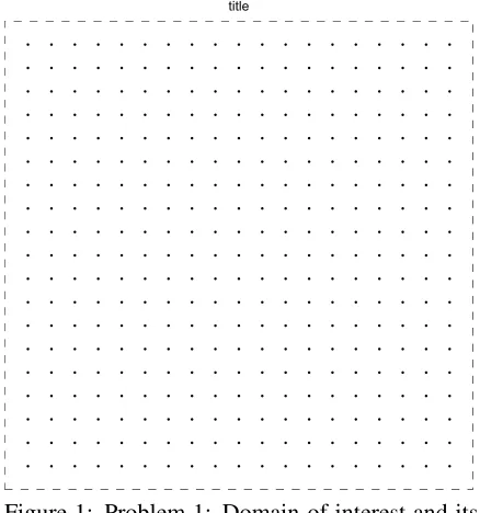
4.1 Problem 1
Consider a simply-supported cross-ply laminate a×a(Figure 1) with four layers 0o/90o/90o/0o under a sinusoidally distributed transverse load
q=q0sin πx
a
sin
πy
a
72 Copyrightc 2007 Tech Science Press CMC, vol.5, no.1, pp.63-77, 2007
[image:10.612.70.289.76.310.2]title
Figure 1: Problem 1: Domain of interest and its discretization.
The material properties are chosen to be [Reddy (2004)]
E1=25E2,ν12=0.25,
G12=G13=0.5E2,G23=0.2E2
A number of uniform densities, namely
{11×11,17×17,21×21,···,41×41}, are
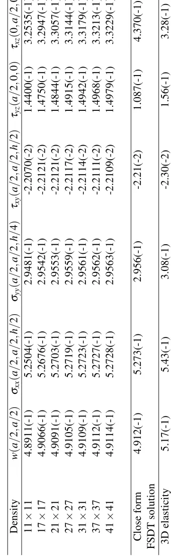
employed to study the convergence behaviour of the present method. The IRBFN results are com-pared with those obtained by the DRBFN method, the close form FSDT solutions [Reddy (2004)] and the 3D-elasticity solutions [Reddy (1984)]. All results are presented in dimensionless forms according to the following relations
w→ 100E2h
3
q0a4
w, (71)
{σxx,σyy,τxy} → qh2
0a2{σxx,σyy,τxy},
(72)
{τyz,τxz} → qh
0a{τyz,τxz}.
(73)
Table 1 presents the results obtained by the DRBFN and IRBFN methods. When compared to the close form solutions using FSDT [Reddy (2004)], it can be clearly seen that the IRBFN method is far superior to the DRBFN method with respect to both accuracy and convergence. For the IRBFN method, the percentage errors are very
small and they are consistently reduced with in-creasing density. It is remarkable that a high de-gree of accuracy is achieved even with a small number of collocation points. For example, at a density of only 21×21, the error of the maximum displacement is about 0.02%. For the DRBFN method, it can be noticed that although the com-puted values of the field variables (i.e. w,ψxand
ψy) are in good agreement with the close form so-lutions, large errors appear in the calculation of their derivatives (e.g. σxx). The DRBFN method is thus very sensitive to noise, and one needs to pay special attention to the process of chosing net-work parameters in order to achieve good accu-racy. On the other hand, the use of integration to construct the RBF approximations significantly stabilizes the solution and enhances the quality of approximation.
Tables 2 and 3 show the full results of the IRBFN method for two different plate thick-nesses, namelya/h=10 anda/h=20. For both cases, very high degrees of accuracy are achieved for the transverse displacement and the in-plane stresses when compared to the close form solu-tions. However, there is some discrepancy be-tween the two solutions for the transverse shear stresses τyz and τxz. It can be seen that the present results are much closer to the 3D elas-ticity solutions. This is due to the fact that the IRBFN method uses the 3D equilibrium equations rather than the constitutive equations for comput-ing these values. Figure 2 shows the distribution of transverse shear stresses through the thickness of the plate obtained by the present method.
4.2 Problem 2
The present method is further verified through the solution of a composite plate with a curved geom-etry. A clamped circular plate with radiusRunder a uniform loadq is considered here. The set of material properties is chosen as follows
E1=5.6×10⁶,E2=1.2×10⁶,ν12=0.26,
G12=G13=G23=0.6×10⁶
The laminate is unidirectional with fibers oriented atθ=0owith respect to the global coordinates. A wide range of the radius-to-thickness ratio,R/h=
0 0.05 0.1 0.15 0.2 0.25 0.3 0.35 í0.5
í0.4 í0.3 í0.2 í0.1 0 0.1 0.2 0.3 0.4 0.5
xlabel
ylabel
0 0.02 0.04 0.06 0.08 0.1 0.12 0.14 0.16 0.18 0.2 í0.5
í0.4 í0.3 í0.2 í0.1 0 0.1 0.2 0.3 0.4 0.5
xlabel
[image:11.612.78.293.70.432.2]ylabel
Figure 2: Problem 1,a/h=10, 41×41: The dis-tribution of transverse shear stresses through the thickness of the plate using 3D equilibrium equa-tions.
The present method does not require any underly-ing mesh. Nodes can thus be located in a flex-ible way. If one uses Cartesian-grid nodes to represent non-rectangular/irregular domains, the computational cost of generating data points can be significantly reduced. This discretization ap-proach is generally recommended for use. For the present problem, the circular plate is first embed-ded in a square domain and the extenembed-ded domain is then discretized using a Cartesian grid, i.e. an array of straight lines that run parallel to thex− and y−axes. The interior points are defined as grid points inside the analysis domain, while the boundary points are generated by the intersection of the grid lines with boundaries. Grid nodes
out-side the analysis domain are removed from the computations (Figure 3).
[image:11.612.323.540.118.340.2]title
Figure 3: Problem 2: Domain of interest and its discretization.
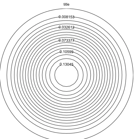
title
0.13045 0.10599 0.073377 0.032612 0.008153
Figure 4: Problem 2: Contour plot of the displace-ment of the plate using a density of 37×37.
[image:11.612.325.539.413.636.2]74 Copyrightc 2007 Tech Science Press CMC, vol.5, no.1, pp.63-77, 2007
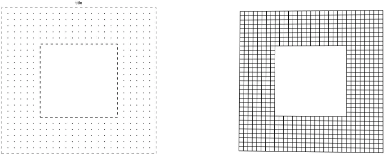
[image:12.612.79.465.74.229.2]title
Figure 5: Problem 3: Discretizations by IRBFN (left) and FEM (S8R elements) (right).
w
[image:12.612.112.456.279.423.2]title
Figure 6: Problem 3: Displacement atz=h/2 obtained by IRBFN (left) and FEM (right).
The central displacement of the plate is non-dimensionalized by a factor of D/qR4 with D= 3(D11+D22) +2(D12+2D66). Table 4 lists the
central displacement of the plate. The corre-sponding results obtained by FEM and the exact solution corresponding to the special case of thin plate [Wilt, Saleeb, and Chang (1990)] are also included for comparison. It is clearly indicated that the present method yields a very high order of accuracy. For example, atR/h=16.67, at least 4 decimal digits remain unchanged when densi-ties are greater than 21×21. However, when the thickness is reduced, higher densities are required to obtain a converged solution. This is probably due to the fact that the thick-plate theories are used here. The results obtained are in good agree-ment with the FEM results, and they approach the thin-plate exact solution with decreasing thick-ness. The typical distribution of the displacement
obtained by the present method is displayed in Figure 4.
4.3 Problem 3
The results obtained in exampples 1 and 2 have clearly demonstrated the excellent accuracy achieved by the present method. It is believed therefore that the IRBFN method can now be confidently used to analyse non-trivial problems. Thus in this example, a plate similar in lamina lay-out to the one in Problem 1 with a cut-lay-out square holea/2×a/2 is analyzed under a uniform pres-sureq0. Good convergence is achieved, as shown
in Table 5, with a shear correction factor of 5/6 which is most suitable for isotropic plates.
a)σxx
title
b)σyy
title
c)τxy
[image:13.612.83.467.80.579.2]title
Figure 7: Problem 3: In-plane stresses atz=h/2 obtained by IRBFN (left) and FEM (right).
[image:13.612.316.461.97.402.2]Abaqus [Hibbitt, Karlsson, and Sorenson (2006)]. Figure 5 shows discretizations by the IRBFN and FEM. In the FEM solution, an eight-node conven-tional shell element with reduced integration and six degrees of freedom per node is used. How-ever, the commercial software ABAQUS does not reveal the value of the shear correction factor for
76 Copyrightc 2007 Tech Science Press CMC, vol.5, no.1, pp.63-77, 2007 5 Concluding Remarks
The meshless IRBFN method is applied to the static analysis of the bending behaviour of mod-erately thick laminated composite plates. Differ-ent geometries and boundary conditions are con-sidered. The RBFN methods require only a min-imum amount of effort to implement as its for-mulation is based on strong form/point colloca-tion, and its “shape functions” are given in an-alytic forms. Unlike the DRBFN, the construc-tion of IRBFN approximaconstruc-tions is based on in-tegration rather than conventional differentiation, which significantly stabilizes the solution and im-proves the accuracy of the numerical results. In contrast to the spectral collocation method, the IRBFN does not require an underlying mesh. For efficiency, Cartesian grids are employed to gener-ate the interpolating points representing the analy-sis domain. Numerical results obtained show that the method attains good accuracy and fast con-vergence for both rectangular and non-rectangular plates.
Acknowledgement: This research was sup-ported by the Australian Research Council
References
Atluri, S. N.; Shen, S. P. (2002): The mesh-less local Petrov-Galerkin (MLPG) method. Tech. Science Press.
Bert, C.; Chen, T.(1978): Effect of shear defor-mation on vibration of antisymmetric angle-ply laminated rectangular plates. International Jour-nal of Solids and Structures 1978; 14:, vol. 14, pp. 465–473.
Haykin, S.(1999): Neural Networks: A Com-prehensive Foundation. Prentice-Hall.
Hibbitt; Karlsson; Sorenson(2006): Abaqus (version 6.6-1). Hibbitt, Karlsson & Sorenson Inc., Pawtucket, RI, USA.
Kansa, E. (1990): Multiquadrics- A scat-tered data approximation scheme with applica-tions to computational fluid-dynamics-II. Solu-tions to parabolic, hyperbolic and elliptic partial
differential equations. Computers and Mathemat-ics with Applications, vol. 19, pp. 147–161.
Liu, G.(2003): Mesh Free Methods: Moving beyond the Finite Element Method. CRC Press.
Liu, P.; Zhang, Y.; Zhang, K.(1994): Bending Solution of high order refined shear deformation theory for rectangular composite plates. Interna-tional Journal of Solids and Structures, vol. 31, pp. 2491–2507.
Madych, W.; Nelson, S. (1988): Multivariate interpolation and conditionally positive definite functions. Approximation Theory and its Appli-cations, vol. 4, pp. 77–89.
Madych, W.; Nelson, S. (1990): Multivariate interpolation and conditionally positive definite functions, II. Mathematics of Computation, vol. 54, pp. 211–230.
Mai-Duy, N.; Tanner, R. (2005): Computing non-Newtonian fluid flow with radial basis func-tion networks. International Journal for Numer-ical Methods in Fluids, vol. 48, pp. 1309–1336.
Mai-Duy, N.; Tran-Cong, T. (2001): Numeri-cal solution of differential equations using multi-quadric radial basis function networks. Neural Networks, vol. 14, pp. 185–199.
Mai-Duy, N.; Tran-Cong, T.(2003): Approxi-mation of function and its derivatives using radial basis function networks. Applied Mathematical Modelling, vol. 27, pp. 197–220.
Mai-Duy, N.; Tran-Cong, T. (2005): An effi-cient indirect RBFN-based method for numerical solution of PDEs. Numerical Methods for Partial Differential Equations, vol. 21, pp. 770–790.
Mai-Duy, N.; Tran-Cong, T.(2006): Solving bi-harmonic problems with scattered-point discreti-sation using indirect radial-basis-function net-works. Engineering Analysis with Boundary El-ements, vol. 30, pp. 77–87.
Pandya, B.; Kant, T.(1988): Flexural analysis of laminated composites using refined higher-order C0 plate bending elements. Computer Methods in Applied Mechanics and Engineering, vol. 66, pp. 173–198.
Park, J.; Sandberg, I. (1991): Universal ap-proximation using radial basis function networks. Neural Computation, vol. 3, pp. 246–257.
Park, J.; Sandberg, I. (1993): Approximation and radial basis function networks. Neural Com-putation, vol. 5, pp. 305–316.
Reddy, J.(1984): A simple higher order theory of laminated composite plates. Journal of Applied Mechanics, vol. 51, pp. 745–752.
Reddy, J. (2004): Mechanics of laminated composite plates and shells. Theory and analysis. CRC Press.
Reddy, J.; Chao, W. (1981): A comparison of closed-form and finite-element solutions of thick laminated anisotropic rectangular plates. Nuclear Engineering and Design, vol. 64, pp. 153–167.
Srinivas, S.; Rao, A. (1970): Bending, vibra-tion and buckling of simply supported thick or-thotropic rectangular plates and laminates. Inter-national Journal of Solids and Structures, vol. 6, pp. 1463–1481.
Wang, Y.; Tarn, J.(1994): A three-dimensional analysis of anisotropic inhomogeneous and lami-nated plates. International Journal of Solids and Structures, vol. 31, pp. 497–515.
Whitney, J.; Pagano, N.(1970): Shear deforma-tion in heterogeneous anisotropic plates. Jour-nal of Applied Mechanics 1970; 37:, vol. 37, pp. 1031–1036.