Computing Non-Newtonian Fluid Flow With Radial
Basis Function Networks
N. Mai-Duy
∗and R.I. Tanner
School of Aerospace, Mechanical and Mechatronic Engineering,
The University of Sydney, NSW 2006, Australia
Submitted to
Int. J. Numer. Meth. Fluids, 27/9/2004; revised 17/2/2005
SUMMARY
This paper is concerned with the application of radial basis function networks (RBFNs)
for solving non-Newtonian fluid flow problems. Indirect RBFNs, which are based on an
integration process, are employed to represent the solution variables; the governing
dif-ferential equations are discretized by means of point collocation. To enhance numerical
stability, stress-splitting techniques are utilized. The proposed method is verified through
the computation of the rectilinear and non-rectilinear flows in a straight duct and the
ax-isymmetric flow in an undulating tube using Newtonian, power-law,
Criminale-Ericksen-Filbey (CEF) and Oldroyd-B models. The obtained results are in good agreement with
the analytic and benchmark solutions.
KEY WORDS: radial basis function network; non-Newtonian fluid; straight duct;
sec-ondary flow; undulating tube.
1
Introduction
Continuum mechanics problems often lead to a set of partial differential equations (PDEs)
together with a set of boundary conditions through the process of mathematical modelling.
For most problems, discretization techniques are required to reduce complex systems of
PDEs to systems of algebraic equations. Principal discretization methods include the
finite-difference method (FDM), the finite-element method (FEM), the boundary-element
method (BEM), the finite-volume method (FVM) and the spectral method. Each method
has advantages over the others for certain classes of problems. They have achieved a lot
of success in solving many engineering and science problems. In FEMs and FVMs, any
continuous quantity is approximated by a set of piecewise continuous functions defined
over a finite number of subdomains identified as elements or control volumes, i.e., mesh.
problems with complex geometries, free surfaces or moving boundaries.
The development of numerical methods without using a mesh (meshless or meshfree
meth-ods) for the solution of PDEs has been an active research area recently. As the name
suggests, there may not be any connectivity requirements between data points, leading
to an easy process of numerical modelling. A comprehensive review of meshless methods
can be found in [1-4]. Based on the criterion of a computational formulation, they can be
divided into two categories: a) those based on the approximation of the strong form of
PDEs, e.g., the smoothed particle hydrodynamics [5] and b) those based on the
approxi-mation of the weak form/inverse statement of PDEs, e.g., the reproducing kernel particle
method [6]. On the other hand, based on the criterion of a mesh requirement, they can
be classified into a) the so-called truly meshless methods (no mesh is involved at all), e.g.,
the meshless local Petrov-Galerkin method [7] and the local radial point interpolation
method [8], and b) the so-called meshless methods (some mesh is still needed for either
the interpolation of solution variables or the integration of weak form/inverse statement),
e.g., the element free Galerkin method [9].
RBFNs, which can be regarded as scattered data approximation schemes, have found
applications in many disciplines. A function to be approximated and its derivatives can
be represented by direct RBFNs (DRBFNs) based on a differentiation process [10] or
by indirect RBFNs (IRBFNs) based on an integration process [11]. The application of
RBFNs for the numerical solution of PDEs was first reported by Kansa [12]. Since then,
it has received a great deal of attention from the research community. A great number
of publications are available in the literature, e.g., for a convergence proof and error
bound [13], the numerical solution of potential problems [14-18], high-order differential
equations [19,20], Kirchhoff plate bending problems [21] and viscous-fluid-flow problems
[22,23]. In a standard RBFN-based method, all dependent variables are first approximated
by global RBFNs, and the governing equations are then discretized in the strong form
elements—throughout a volume, which can be randomly distributed, to approximate the
field variables; hence, they can be regarded as truly meshless methods. Since RBFNs fall
into the category of high-order approximation, another attractive feature lies in accuracy
for a given number of data points. Furthermore, they require only a minimum amount of
effort to implement.
This paper is concerned with the development of IRBFNs for the numerical solution
of non-Newtonian fluid flow problems. Unlike constitutive models of Newtonian fluids,
models of non-Newtonian fluids are nonlinear, making their computation difficult. For
generalized Newtonian fluids, e.g., power-law fluid, the viscosity function depends on the
rate of deformation of the fluid; while for viscoelastic fluids, e.g., CEF and Oldroyd-B
fluids, the stress in the liquid depends not only on the present boundary data, but also
on the history of the strain [24]. The present method is verified by its applications to the
simulation of Newtonian, power law, CEF and Oldroyd-B fluids flowing through ducts of
constant and variable cross sections that are induced by axial pressure drop. The obtained
results are in good agreement with the analytic and benchmark solutions.
The remainder of the paper is organized as follows. In section 2, the governing equations
are given. In section 3, the numerical formulation of non-Newtonian fluid flows using
RBFNs is presented. The rectilinear and non-rectilinear flows in a straight duct and the
axisymmetric flow through an indefinitely long undulating tube are simulated in section
4. Section 5 gives some concluding remarks.
2
Governing equations
the forms
ρ
∂v
∂t +v.∇v
= ∇.σ, x∈Ω, (1)
∇.v = 0, x∈Ω, (2)
wherex is the position vector,t the time, Ω the domain of interest,v the velocity vector and σ the stress tensor. The stress tensor can be written as
σ =−pI+τ, (3)
where p is the pressure, I the unit tensor and τ the extra stress tensor. In the present work, the Newtonian, power-law, CEF and Oldroyd-B models are considered with the
extra stress tensors defined as
τ =ηγ˙, (Newtonian model), (4)
τ =η( ˙γ)γ˙, η( ˙γ) =k|γ˙|n−1, (power-law model), (5)
τ =η( ˙γ)γ˙ −1
2Ψ1 Δγ˙
Δt + Ψ2γ˙.γ˙, η( ˙γ) = k|γ˙|
n−1, (CEF model), (6)
τ =ηsγ˙ +S, S+λΔS
Δt =ηγ˙, (Oldroyd-B model), (7)
where γ˙ is the rate of deformation tensor,
˙
γ =∇v+∇vT;
˙
γ is the scalar magnitude of γ˙,
˙
γ =(1/2)tr(γ˙.γ˙),
solvent-contributed stress (ηs the solvent viscosity); S the polymer-contributed stress; λ
the relaxation time; and Δ[]Δt the upper convected derivative,
Δ[] Δt =
∂[]
∂t + (v.∇)[]− ∇v
T.[]−[].∇v.
3
Radial basis function networks
A function y, to be approximated, can be represented by an RBFN as follows [25]
y(x)≈f(x) =
m
i=1
w(i)g(i)(x), (8)
where superscript denotes the elements of an RBFN,xthe input vector,m the number of RBFs,{w(i)}mi=1 the set of network weights to be found, and{g(i)(x)}mi=1 the set of RBFs.
According to Micchelli’s theorem, there is a large class of RBFs, e.g., multiquadrics,
inverse multiquadrics and Gaussian functions, whose design matrices (interpolation
ma-trices) obtained from (8) are always invertible provided that the data points are distinct.
This is all that is required for nonsingularity of design matrices, whatever the number
of data points and the dimension of problem [26,25]. It has been proved that RBFNs
are capable of representing any continuous function to a prescribed degree of accuracy
in the Lp norm, p ∈[1,∞] [27,25]. On the other hand, according to the Cover theorem, the higher the number of neurons (RBFs) used, the more accurate the approximation
will be [28], indicating the property of “mesh convergence” of RBFNs. These important
theorems can be seen to provide the theoretical basis for the design of RBFNs to the field
of numerical solution of PDEs.
In solving PDEs with RBFNs, multiquadrics (MQ) and thin plate splines (TPS) are widely
general, they tend to result in the most accurate approximation. The MQ-approximation
scheme gives exponential convergence with the refinement of spatial discretization. In
practice, the MQ-RBFN solution can be strongly influenced by the RBF width (shape
parameter), and how to choose the best value of this free parameter is still open. On the
other hand, TPSs do not involve the adjustable shape parameter. Like the MQ case, high
accuracy can be obtained using relatively low data densities. However, TPSs possess only
linear convergence [18]. In the present work, these RBFs are implemented, whose forms
are
g(i)(x) =
(x−c(i))T(x−c(i)) +a(i)2 (MQ), (9)
g(i)(x) = (x−c(i))T(x−c(i)) log
(x−c(i))T(x−c(i))
(TPS), (10)
where c(i) and a(i) are the centre and the width of the ith RBF, respectively, and super-scriptT denotes the transpose of a vector. To make the training process simple, the set of centres is chosen to be the same as the set of collocation points, i.e.,{c(i)}mi=1 ≡ {x(i)}pi=1
with m=p, and the width a(i) is computed using the following relation
a(i)=βd(i), (11)
where β is a positive scalar and d(i) is the minimum of distances from the ith center to its neighbours. Relation (11) allows the MQ width a to be broader in the area of lower data density and narrower in the area of higher data density in order to achieve a certain
amount of response overlap between each RBF and its neighbours (“P nearest neighbour”
3.1
Direct approach
In the DRBFN approach, the RBFN (8) is utilized to represent the original function y; subsequently, its derivatives are computed by differentiating (8) as
y(x) ≈ f(x) =
m
i=1
w(i)g(i)(x), (12)
∂y(x)
∂xj ≈
∂f(x)
∂xj =
∂mi=1w(i)g(i)(x)
∂xj =
m
i=1
w(i)h(i)(x), (13)
∂2y(x)
∂x2j ≈
∂2f(x)
∂x2j =
∂mi=1w(i)h(i)(x)
∂xj =
m
i=1
w(i)¯h(i)(x), (14)
where subscript j denotes the scalar components of a vector; h(i)(x) = ∂g(i)(x)/∂xj and ¯
h(i)(x) =∂h(i)(x)/∂xj are new derived basis functions for the approximation of the first-and the second-order derivatives of the original function y, respectively.
3.2
Indirect approach
In this approach, RBFNs are used to represent the highest-order derivatives of a function
y, e.g., ∂2y/∂x21 and ∂2y/∂x22—the highest ones under consideration here. Lower-order derivatives and finally the function itself are then obtained by integrating those RBFNs
as follows
∂2y(x)
∂x2j ≈
∂2f(x)
∂x2j =
m
i=1
w([xi)
j]g
(i)(x), (15)
∂y(x)
∂xj ≈
∂f(x)
∂xj =
m+q1
i=1
w([xi)
j]H
(i)
[xj](x), (16)
y(x) ≈ f(x) =
m+q2
i=1
w([xi)
j]
¯
H[(xi)
j](x). (17)
approximate a set of nodal integration constants; q2 = 2q1; H[(xi)
j]=
g(i)dxj and ¯H[(xi)
j] =
H(i)dxj (i = 1,2,· · · , m) are new derived basis functions for the approximation of the first-order derivative and the original function y, respectively. For convenience of presentation, the new centres and their associated known basis functions in subnetworks
are also denoted by the notationsw(i) andH(i)(x) ( ¯H(i)(x)), respectively, but withi > m.
Since integration is a smoothing operation, the approximating functions obtained by the
IRBFN method are expected to be much smoother than those by the DRBFN method.
Previous findings showed that the former performs better than the latter in terms of
accuracy and convergence rate [11].
The theoretical justification for applying RBFNs to solve general PDEs with RBFNs has
not been established yet [17]. Recently, Franke and Schaback [13] gave a convergence
proof and error bound for methods solving constant-coefficient PDEs by collocation using
DRBFNs. A formal theoretical proof of the superior accuracy of the IRBFN method and
the non-singularity of IRBFN matrices cannot be offered at this stage.
Unlike FEMs and BEMs, where the integration process is used to reduce the order of
the continuity required for the variables, the integration process in the IRBFN method
is employed solely to obtain new basis functions from RBFs. In the context of meshless
methods, all relevant integrals in the IRBFN method using MQs and TPSs are determined
analytically, leading directly to a truly meshless method; while the integration of the
weak form associated with FEM or the inverse statement associated with BEM must be
computed numerically, and hence they require some special treatments, e.g., using local
weak form/local inverse statement, to achieve a mesh-free feature.
When the problem dimension N is greater than 1, the size of a system of equations obtained by the IRBFN approach is aboutN times as big as that by the DRBFN approach. Thus, it is necessary to make a prior conversion of the multiple spaces of network weights
The evaluation of (15)-(17) at a set of collocation points {x(k)}mk=1 yields
f,jj = Gw[xj], (18)
f,j = H[xj]w[xj], (19)
f = H¯[xj]w[xj], (20)
where G, H and H¯, whose rows can be seen in (28), (27) and (26), are the design
matrices associated with the approximation of the second-order derivative, the first-order
derivative, and the function, respectively; w[xj] the set of network weights in the xj
direction to be found; f = {f(x(k))}mk=1; f,j = {∂f∂x(x(k))
j }
m
k=1 and f,jj = {∂2f∂x(x2(k))
j }
m k=1.
For the purpose of computation, the two matrices G and H are augmented using
zero-submatrices so that they have the same size as the matrix H¯. By solving (20) using the
general linear least squares method, the set of network weights can be expressed in terms
of the nodal function values as
w[xj]=H¯−[x1
j]f, (21)
whereH¯−[x1
j] is the Moore-Penrose pseudoinverse, and the dimensions ofw,H¯
−1
[xj]and f are
respectively (m+q2)×1, (m+q2)×m and m×1. Substitution of (21) into (18)-(20) yields
f,jj = G ¯H−[x1
j]f, (22)
f,j = H[xj]H¯−[x1
j]f, (23)
f = H¯[xj]H¯−[x1
j]f. (24)
Cross derivatives ∂f2(x)/∂xi∂xj can be straightforwardly computed by using the design matrices associated with the first-order derivatives (23). Although the order of
error,
∂2f ∂xi∂xj =
1 2 ∂ ∂xi ∂f ∂xj + ∂ ∂xj ∂f ∂xi ,
f,ij = 1 2
H[xi]H¯−[x1
i]
H[xj]H¯−[x1
j]f
+H[xj]H¯−[x1
j]
H[xi]H¯−[x1
i]f
. (25)
Expressions of f and its derivatives at an arbitrary pointx can be given by
f(x) = 1
N N j=1 ¯
H[(1)x
j](x),· · · , ¯
H[(xm+1)
j] (x),· · · , ¯
H[(xm+q1+1)
j] (x),· · ·
¯ H−[x1
j]f
, (26)
∂f(x)
∂xj =
H[(1)x
j](x),· · · , H
(m+1)
[xj] (x),· · · ,0,· · ·
¯ H−[x1
j]f, (27)
∂2f(x)
∂x2j =
g[(1)x
j](x),· · · ,0,· · · ,0,· · ·
¯ H−[x1
j]f, (28)
∂2f(x)
∂xi∂xj =
1 2(
H[(1)x
i](x),· · · , H
(m+1)
[xi] (x),· · · ,0,· · ·
¯ H−[x1
i]
H[xj]H¯−[x1
j]f
+
H[(1)x
j](x),· · · , H
(m+1)
[xj] (x),· · · ,0,· · ·
¯ H−[x1
j]
H[xi]H¯−[x1
i]f
), (29)
where N is the dimension of the problem. In (26), the approximate function f at x is taken to be the average value of f[xj](x)’s due to numerical error.
From (26)-(29), a function y and its derivatives are now expressed in terms of function values rather than in terms of network weights. As a result, in solving PDEs, the present
IRBFN method leads to a system of equations whose size is approximately equal to that of
the DRBFN method, irrespective of the problem dimension. The process of transforming
network-weight space into physical space completely eliminates the problem of the large
system/final-matrix size of the IRBFN method. However, the IRBFN method requires
3.3
The numerical IRBFN formulation
Each dependent variable and its derivatives in the governing equations (1)-(7) can be
approximated by RBFNs using either (12)-(14) for the DRBFN approach or (26)-(29)
for the IRBFN approach. The closed-form representations obtained are substituted into
the governing equations, and the system of PDEs is then discretized by means of point
collocation. The RBFN solution thus satisfies the governing equations pointwise rather
than in an average sense. In the present work, only the IRBFN approach is employed. In
contrast to previous works dealing with potential and viscous flow problems [15,22], the
present IRBFN formulation is expressed in terms of the nodal variable values. For the
elliptic momentum equations, one only needs to enforce these equations at interior points
because the velocity boundary conditions are prescribed along the entire boundary. For
the hyperbolic constitutive equations, the IRBFN formulation is demonstrated through
one equation in (7), e.g., forSzz,
nip
i=1
{Szz(i)+λ(v(ri)
m
j=1
H[r]H¯−[r1]
[i,j]S (j)
zz +vz(i) m
j=1
H[z]H¯−[z1]
[i,j]S (j)
zz
−2Srz(i)
m
j=1
H[r]H¯−[r1]
[i,j]v (j)
z −2Szz(i) m
j=1
H[z]H¯−[z1]
[i,j]v (j)
z )
−2η
m
j=1
H[z]H¯−[z1]
[i,j]v (j)
z }2 →0, (30)
where (r, θ, z) denotes the cylindrical polar coordinates, nipthe number of interior points,
m the number of centres excluding centres on the tube wall and [i, j] the element located at row i and column j of a matrix. On the tube wall, (7) is reduced to a set of algebraic equations because of ΔS/Δt = 0; consequently, the stress components can be easily computed. In this regard, for solving hyperbolic equations, one may not need to include
the tube-wall points in the set of centres. Other equations in (7) can be discretized in a
4
Numerical examples
Axial-pressure-drop-induced flows in a straight duct and in a “wiggly” tube using
Newto-nian, power-law, CEF and Oldroyd-B fluid models are simulated to study the performance
of the IRBFN method,.
4.1
Rectilinear and non-rectilinear flows in a straight duct
MQs are employed to compute flows of a power-law fluid through circular and non-circular
tubes, while TPSs are used to simulate the flow of a viscoelastic fluid through a square
duct. For simplicity, in the MQ-based approximation scheme, the factor β is chosen to be unity. To enhance numerical stability, a stress-splitting formulation is employed. The
resulting nonlinear system of equations is solved by a decoupled approach, where a
Picard-type iteration scheme is utilized to render nonlinear terms linear. At each iteration, a
perturbed Newtonian problem and a constitutive model are solved in two sequential steps.
For a given kinematics, a pseudo-body force field is obtained by solving the constitutive
model. The kinematics are then updated by solving the momentum and the continuity
equations. The procedure is iterated until a stopping criterion is satisfied. Hence, an
attractive feature of this technique lies in the small requirement of computer memory.
For low values of n, it is necessary to relax the iterative process by applying a relaxation factor to the field variables according to, e.g., for a component velocity vj,
where α is the relaxation factor (0 < α ≤ 1) and superscript k indicates the current iteration. Convergence measure (CM) at thekth iteration is defined as
CM =
Nj=1
m
i=1
vjk(x(i))−vjk−1(x(i))2
N
j=1
m
i=1
vkj(x(i)))2 ,
where N is the problem dimension and m the number of collocation points.
4.1.1 Fully developed laminar flow of power-law fluid in a straight circular
pipe
For the flow of a power-law fluid in a straight circular pipe (vr = 0; vθ = 0; vz =vz(r)), the continuity equation (2) is automatically satisfied, and the momentum equation (1)
can be reduced to
1
r ∂ ∂r
ηr∂vz
∂r
− ∂p
∂z = 0, (32)
η=k∂vz ∂r
n−1, (33)
on the domain 0< r < R, which is solved subject to the boundary conditions
∂vz
∂r = 0, at r= 0, (34)
vz = 0, at r =R. (35)
The exact solution of this problem is
vze = n
n+ 1
−∂p/∂z
2k
1/n
R(n+1)/n
1−
r R
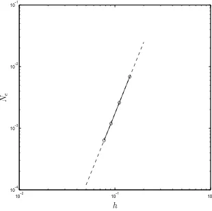
Since the exact solution is available, the accuracy of a numerical solution can be measured
via the norm of relative errors of the solution as follows
Ne=
m
i=1[vze(x(i))−vz(x(i))]2
m
i=1vze(x(i))2
, (36)
where vz and vze are the calculated and the exact solutions, respectively.
The governing equation (32) can be rewritten as
η∂
2v
z
∂r2 + ∂η ∂r ∂vz ∂r − ∂p ∂z + η r ∂vz
∂r = 0. (37)
This equation is widely used in FDMs. For generalized Newtonian fluids, the viscosity η
is a function of the velocity field. As a result, a system matrix obtained from (37) varies
and needs to be inverted at each iteration.
The power-law fluid implies an infinite viscosity when the shear rate ˙γ vanishes; some special treatments for terms involving η are required. Young and Wheeler [29] treated this infinity by using a truncation procedure. A large value of the viscosity, namelyηmax, is given. Ifη does not exceed ηmax, then the computed value is accepted. Otherwise, η is set equal to ηmax. For collocation methods, one can simply treat this singularity by not applying the governing equations at points of infinite viscosity. In the present work, the
extra stress tensor is decomposed into two components
τ = ([η−η0] +η0)γ˙ = [η−η0]γ˙ +η0γ˙. (38)
It is obvious that η0 can be chosen arbitrarily. Substitution of (38) into (32) yields
η0
∂2vz ∂r2 +
1 r ∂vz ∂r − ∂p ∂z + ∂ ∂r
[η−η0]∂vz
∂r
+ [η−η0]
r
∂vz ∂r
= 0, (39)
A system matrix obtained from (39) depends only on the geometry and hence needs to
be inverted only once.
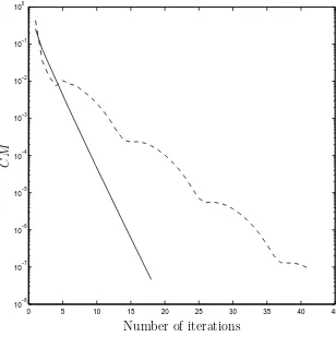
The question here is how to choose an optimum η0. Two studies are conducted. Firstly,
η0 is chosen to be the Newtonian-like viscosity corresponding to n = 1 (η0 = ηN =
k); secondly, η0 is taken to be the average viscosity of the previous iteration (η0 = ¯η). Numerical experience shows that the case η0 = ¯η outperforms the case η0 =ηN regarding the convergence behaviour of an iterative procedure (Figure 1) and the achievement of a
low-power-law-index solution.
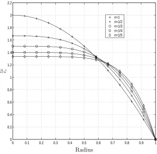
A wide range of n varying from 1 to 1/5 is considered. All values of k, −∂p/∂z and R
are chosen to be unity. The obtained results are displayed in Figure 2, where the velocity
component vz is normalized with the average velocity ¯vz = 2π01rvz(r)dr in which the integral is computed using Simpson rule. Good agreement is seen between the exact and
the computed solutions. For example, at n = 1/5, the method achieves a small error-norm,Ne = 6.4e−4, using 13 collocation points. “Mesh convergence” is shown in Figure 3, where the IRBFN solution converges apparently as O(h3.85) in which h is the centre spacing. As mentioned earlier, the MQ width can critically affect the performance of
MQ-RBFNs. However, there is no general theory yet for determining the best value of the
MQ width. Consequently, in practice, it is difficult to achieve exponential convergence,
even for the case of function approximation.
4.1.2 Fully developed laminar flow of power-law fluid in a square duct
Computing the flow in a square duct is known to be more complicated than
comput-ing the flow in a circular pipe flow. A two-dimensional computation is required. For
non-Newtonian fluids, exact solutions are not available; one needs to resort to numerical
methods. Hartnett and Kostic [30] gave a comprehensive review on the heat transfer
rect-angular duct. The flow was simulated by a number of numerical methods, for example,
a variational principle [31], FDM [32] and FEM[33]. It was indicated that convergence
often fails for n <0.4.
It is plausible to assume that the flow of an inelastic fluid in a straight duct is rectilinear,
i.e., vx = 0, vy = 0 and vz = vz(x, y). The governing equations (1)-(3) and (5) can be reduced to
∂ ∂x
η∂vz
∂x
+ ∂
∂y
η∂vz ∂y
− ∂p
∂z = 0, (40)
η=k ∂vz ∂x 2 + ∂vz ∂y
2n−1 2
. (41)
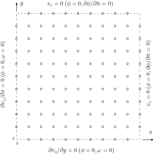
A stress-splitting formulation is employed here to enhance numerical stability and reduce
computational effort. Owing to the symmetry, only a quarter of the 2D domain is
consid-ered (Figure 4). The domain of interest, ∂p/∂z and k are chosen to be 0.5×0.5, -1 and 1, respectively. Special attention is given to the treatment for the Neumann condition
∂vz/∂n¯ (¯n the coordinate normal to the boundary). The present method implements this type of boundary condition as follows. Along the two sides x = 0 and y = 0, normal derivatives∂vz/∂n¯ are given, and hence the task now is to express the nodal values of vz
along these sides in terms of the interior nodal variable values. This can be achieved by
solving the following subsystem of equations
∂vz(x(i))
∂n¯ =
m
j=1
H[xn]H¯−[x1
n]
[i,j]v (j)
z , (42)
where x(i) = {(x = 0, y),(x, y = 0)}. Making use of the results obtained from (42) and the Dirichlet condition (vz = 0 along the wall), a square system of equations is obtained with the unknowns being only the interior variable values. Once the system of equations
Again, the case η0 = ¯η yields faster convergence than the case η0 = ηN. For example, at n = 0.8 and α = 0.1, it takes about 10 and 35 iterations to obtain convergence (CM <1.e−6) for η0 = ¯η and η0 = ηN, respectively. Furthermore, low values of n, at least 1/5, are simulated successfully with the former, while the latter is only able to obtain
convergence for 1 ≥ n ≥ 0.4. Due to the fact that the solving procedure is Picard-type iterative, an initial solution can greatly affect convergence behaviour. Here, the computed
solutions at greater values of n are chosen to be initial solutions. Figure 5 presents the plot of convergence measure versus iteration for several initial solutions. It can be seen
that a closer initial solution yields faster convergence.
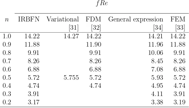
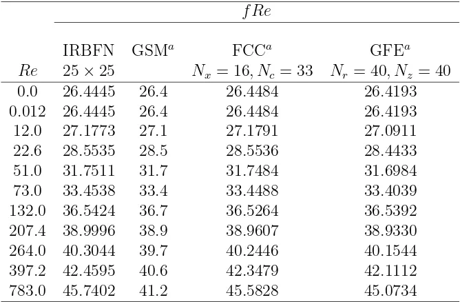
Another important quantity associated with this type of flow is the friction factor-Reynolds
number product, termed f Re, which describes the relationship between flow rate and pressure drop. For the problem under consideration, the quantity f Re has the form
f Re= 1
2¯vnz, (43)
where ¯vz is the average velocity in the flow direction, defined as
¯
vz = 4
0.5
0
0.5
0
vz(x, y)dxdy,
in which the double integral can be evaluated using Simpson quadrature. Based on
the Rabinowitsch-Mooney equation, Kozicki, Chou and Tiu [34] derived an approximate
expression of the friction factor defined as, e.g., for a square duct,
f Re= 23n+1
0.6771 +0.2121
n n
.
Results for the friction factor obtained by the present method and other methods [31-34]
are summarized in Table 1. These predictions are in good agreement over a wide range
4.1.3 Fully developed flow of viscoelastic fluid in a square duct
Viscoelastic fluids possess both viscous and elastic properties. For the fully developed
flow of a viscoelastic fluid through a straight duct, the second normal stress difference is
expected to generate some secondary flow which is transverse to the main flow along the
axis of a duct. However, it does not happen for all cases [24]. For example, the flow is
still rectilinear if the slip surfaces are parallel planes or coaxial circular cylinders; or if
the second normal stress coefficient (Ψ2) is a constant multiple of the viscosity function.
Nevertheless, the appearance of transverse circulations can be seen as a distinguishing
feature of viscoelastic fluids relative to inelastic fluids. As a result, much attention is
paid to the investigation of the development of secondary motions. In earlier studies,
Green and Rivlin [35] examined the flow in a tube of elliptical cross-section, using a
special constitutive equation, and found a weak secondary circulation in each quadrant,
whereas Langlois and Rivlin [36] extended this work for a more general class of fluids.
The secondary flow in a rectangular duct was then studied extensively, for example, using
perturbation approximation [37], FVM [38,39], FDM [40] and FEM [41].
For the purpose of validating the IRBFN method, the present work considers the flow of
a 2% viscarin solution in distilled water through a straight duct of square cross-section
that was studied numerically and experimentally by Gervang and Larson [38]. In view
of the fact that the secondary flow is weak, i.e., the transverse velocity components are
small relative to the main axial velocity component, the fluid can be modelled by the
CEF equation for which rheometric functions are available:
η =kγ˙n−1, k= 8.5P asn, n= 0.37,
Ψ1 =k1γ˙n1, k
1 = 5.96P asn1+2, n1 =−1.35,
Since the fully developed flow is independent of the streamwise coordinate, the governing
equations in a stress-splitting form can be reduced to
ρ
vx∂vx ∂x +vy
∂vx ∂y
= −∂p
∂x +η0
∂2vx ∂x2 +
∂2vx ∂y2
+∂Sxx
∂x + ∂Sxy
∂y , (44) ρ
vx∂vy
∂x +vy ∂vy
∂y
= −∂p
∂y +η0
∂2vy ∂x2 +
∂2vy ∂y2
+ ∂Syx
∂x + ∂Syy
∂y , (45) ρ
vx∂vz
∂x +vy ∂vz
∂y
= −∂p
∂z +η0
∂2vz ∂x2 +
∂2vz ∂y2
+ ∂Szx
∂x + ∂Szy
∂y , (46)
where
S = (η( ˙γ)−η0)γ˙ − 1
2Ψ1 Δγ˙
Δt + Ψ2γ˙.γ˙.
The domain of interest can be reduced to a two-dimensional space and in addition, for
symmetry reasons, only a quarter of the 2D-domain, [0, l/2]×[0, l/2], is considered (Figure 4).
The pressure variable appearing in (44) and (45) is simply treated here by converting the
x andy components of the velocity vector into the stream function φ and the vorticity ω
as
ω = ∂vy
∂x − ∂vx
∂y , (47)
∂φ ∂y =vx,
∂φ
∂x =−vy. (48)
The governing equations (44)-(46) can be reformulated into
∂2φ ∂x2 +
∂2φ
∂y2 +ω = 0, (49)
ρ ∂φ ∂y ∂ω ∂x − ∂φ ∂x ∂ω ∂y
=η0
∂2ω ∂x2 +
∂2ω ∂y2
+∂
2S
xy
∂x2 −
∂2(Sxx−Syy)
∂x∂y − ∂2Sxy
∂y2 , (50) ρ ∂φ ∂y ∂vz ∂x − ∂φ ∂x ∂vz ∂y
=−∂p
∂z +η0
∂2vz ∂x2 +
∂2vz ∂y2
+ ∂Szx
∂x + ∂Szy
The boundary conditions for φ, ω and vz are
φ= 0, ω= 0, ∂vz
∂y = 0, on the liney= 0, (52) φ= 0, ω= 0, ∂vz
∂x = 0, on the linex= 0, (53) φ= 0, ∂φ
∂y = 0, vz = 0, on the liney= l
2, (54)
φ= 0, ∂φ
∂x = 0, vz = 0, on the linex= l
2. (55)
The implementation of the Neumann condition∂vz/∂¯nis similar to the previous problem. It is necessary to generate a computational boundary condition forω at the walls x=l/2 andy =l/2 using the prescribed boundary conditions (∂φ/∂¯n). The process is as follows. In the first step, the vorticity in (49) can be simplified to be
ω = −∂
2φ
∂x2 − ∂2φ ∂y2 =−
∂2φ
∂x2 at the linex= l
2, (56)
ω = −∂
2φ
∂x2 − ∂2φ ∂y2 =−
∂2φ
∂y2 at the liney= l
2. (57)
In the second step, they are written in terms of the first-order derivatives of φ
ω(i) = =−∂
2φ(i)
∂x2 =
m
j=1
GH−[x1]
[i,j]
∂φ ∂x
(j)
at the linex= l
2, (58)
ω(i) = =−∂
2φ(i)
∂y2 =
m
j=1
GH−[y1]
[i,j]
∂φ ∂y
(j)
at the liney= l
2, (59)
and the resulting expressions (58) and (59) are then simplified by taking into account
nodal stream function values, for example, at the boundary point x(i),
∂φ ∂x
(i)
=
m
j=1
H[x]H¯−[x1]
[i,j]φ
(j), (60)
∂φ ∂y
(i)
=
m
j=1
H[y]H¯−[y1]
[i,j]φ
(j). (61)
A computational Dirichlet condition for ω is thus generated and written in terms of the nodal values of φ.
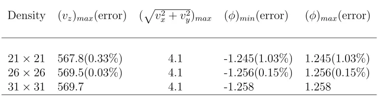
Three sets of uniformly distributed data points, 21×21, 26×26 and 31×31 are
em-ployed. The parameters ∂p/∂z,ρ and l are chosen to be 1.0e5 (P a/m), 0 and 0.004 (m), respectively. The obtained results including the axial velocity, vorticity, secondary
ve-locity vector and second normal stress difference are displayed in Figure 6, which look
feasible when compared to the available solutions in the literature. To study convergence
behaviour of the method, the results at the finest discretization are regarded as the
“ex-act solutions” and the errors at coarser discretizations are then computed relative to the
exact ones. Table 2 shows that errors consistently reduce with an increase in data density.
It can be seen that the transverse velocity components are much smaller than the axial
velocity component.
4.2
Corrugated tube flow
The steady-state axisymmetric non-Newtonian fluid flow through an undulating tube has
received much attention over recent decades for a number of reasons: a) for the evaluation
of constitutive equations, b) for the testing of numerical methods in non-Newtonian flow
calculations and c) for the understanding of viscoelastic effects in flow through porous
media [42]. In the context of numerical computation, this problem was studied by a
vari-ety of numerical methods, for example, the mixed spectral finite-difference methods (the
cylindrical/finite-difference method (PCFD)) [43,42,44], the full pseudospectral method (the Fourier-Chebyshev
collocation method (FCC)) [45], FEM [46] and BEM [47]. The comprehensive results
ob-tained by PSFD, PCFD and FCC can be regarded as the benchmark solutions. There is
no limit point in Weissenberg number for PCFD and PSFD; their numerical calculations
have shown no substantial increase of the flow resistance with increasing flow elasticity.
The local radius of an infinitely long corrugated tube is given by
rw(z) = R(1−sin(2πz/L)), (62)
where rw is the radius at the wall, the dimensionless amplitude of the corrugation, L
the wavelength and R the mean radius of the tube (Figure 7). In addition to , another characteristic dimensionless number is the aspect ratio N, related to the dimensionless wave number l by N = R/L = l/(2π). Owing to the fact that the flow is axisymmetric and periodic, only a reduced domain needs to be considered as shown in Figure 7.
Of interest to the experiments is the flow resistance (friction factor f times Reynolds number in the limit Re→0) defined as
f Re= 2πΔP R
4
L(η+ηs)Q, (63)
where ΔP is the pressure drop per unit cell.
The φ–ω formulation is adopted, where the full governing equations can be found in [48]. The Newtonian, power-law and Oldroyd-B fluid models are considered. For a power-law
fluid, the stress-splitting formulation is employed.
The boundary conditions for flow in a corrugated tube are a) symmetric conditions on
each dependent variable and its normal derivative on the inlet and outlet, i.e.,
φ= 0, ω = 0 (the centreline) (64)
φ= Q 2π,
∂φ ∂n¯ = 0
∂φ ∂z = 0,
∂φ ∂r = 0
(the wall) (65)
φi =φo, ∂φ
i
∂n¯ =
∂φo ∂n¯ , ω
i =ωo, ∂ωi
∂n¯ =
∂ωo
∂n¯ (inlet and outlet), (66)
where ¯n is the coordinate normal to the boundary, Q the flow rate, subscripts i and o
the inlet and outlet, respectively. The implementation of boundary conditions for ω on the tube wall is similar to the previous problem (flow in a square duct) and will not be
repeated here.
Three data densities, namely 17×17, 21×21 and 25×25, are employed (Figure 8). Only
MQs with β= 1 are implemented to study this problem.
4.2.1 Newtonian flow
Creeping flow
The unsymmetric IRBFN collocation method is first tested with the creeping flow of a
Newtonian fluid. Several tube geometries are considered. The flow resistance computed
by the present method is given in Table 3. Results by other methods such as FCC, PSFD,
PCFD and BEM are also included for comparison. Good agreement is obtained for all
test cases.
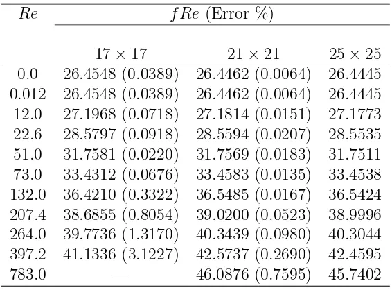
Inertial flow
Consider the inertial flow of a Newtonian fluid through a tube of = 0.3 and N = 0.16. This flow was studied by Lahbabi and Chang [49] using the global Galerkin/spectral
and FCC for a wide range of Re from 0 to 783. For a Newtonian fluid, the nonlinearity is due to the convective term only.
Table 4 shows that errors at coarser densities, which are computed relative to the finest
density, reduce with an increase in data density. The flow resistance obtained by the
present method at the finest density (25×25) and those obtained by the spectral method
and FEM for the above range of Re are presented in Table 5. The present results agree well with the FCC ones. Contour plots of the stream function and the vorticity fields at
Re ={0,22.6,73,397.2} are displayed in Figure 9. The creeping flow field is symmetric about the widest cross section. When a Reynolds number is introduced, the symmetry
is broken. Recirculation starts at a finite Reynolds number. The vortex increases in size
and shifts downstream with an increase in Re.
4.2.2 Inertial flow of power-law fluid
Consider dilute aqueous solution of a polyacrylamide (Dow Separan AP-30) corresponding
to 0.05% polyacrylamide concentrations by weight. The power-law parameters are given
by Deiber and Schowalter [50] as n = 0.54 and k = 1P sn−1. Due to the shear-thinning form of the viscosity, there are steep boundary layers near solid boundaries, leading to
difficulty in computation [42]. The flow of a power-law fluid through an undulating tube
(= 0.3, N = 0.1592), which was simulated by PCFD [42], is considered here.
The Reynolds number and the flow resistance for this problem are respectively defined as
[42]
Re = 2
nπn−2ρQ2−nR3n−4
k , (67)
f Re = 2
nπnΔP R3n+1
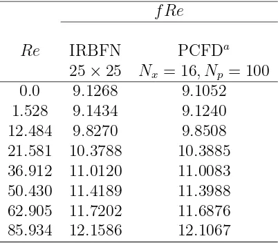
A decoupled approach is adopted to solve the governing equations; the nonlinearity, which
arises from the viscosity function and the convective term, is treated by using a Picard’s
iterative scheme. Results for the flow resistance obtained by the present method are given
in Table 6 together with those obtained by PCFD. The two numerical predictions show
good agreement.
4.2.3 Creeping flow of Oldroyd-B fluid
A coupled approach is adopted. The nonlinearity, which arises from the convected stress
derivatives, is handled by using trust region methods that retain two attractive features,
namely rapid local convergence of the Newtonian iteration method and strong global
convergence of the Cauchy method [51]. The boundary conditions for the stress tensor
are
∂Szz
∂r = 0, Srz = 0, ∂Srr
∂r = 0, ∂Sθθ
∂r = 0 (the centreline) (69) Szzi =Szzo , ∂S
i zz
∂n¯ =
∂Szzo ∂n¯ , S
i
rz =Srzo ,
∂Srzi ∂n¯ =
∂Srzo
∂n¯ · · ·(inlet and outlet). (70)
A Weissenberg number is defined as [43]
W e = λQ
R3. (71)
Along the wall of a tube, all convected stress derivatives vanish, and hence the constitutive
equations are reduced to algebraic equations which can be easily solved pointwise for the
unknown stress tensor.
Along the centreline, the dependent variables will be determined here by imposing the
symmetric conditions directly on the corresponding networks rather than using the usual
L’Hopital’s rule or a simplified form of the governing equations. The detailed
As mentioned earlier, all variables and their derivatives in the present procedure are
expressed as linear combinations of the nodal variable values over the whole domain. Let
f be a dependent variable. The first-order derivative of f with respect to r along the centreline can be written as
f,rc =Hc[r]H¯−[r]1f, (72)
where subscript c denotes the centreline. Making use of the symmetric conditions, (72) becomes
0=Hc[r]H¯−[r]1f. (73)
By solving (73), the centreline values of f can be expressed in terms of the remainder of the nodal values off. A variablef can bevz, Szz, Srr orSθθ. With this treatment, one can avoid to solve ordinary differential equations that are associated with a simplified form
of constitutive equations or to compute higher-order derivatives that are associated with
L’Hopital’s rule. Note that higher-order derivatives lead to larger errors in the context of
function approximation.
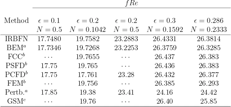
Moderate corrugation amplitude and moderate wavelength (= 0.1, N = 0.16)
The retardation defined as α = η/(ηs+η) is chosen to be 0.15, which was used in [43]. Convergence can be obtained up to high values of the Weissenberg number, at least of
about 30 (Figure 10). For the range ofW efrom 0 to 20, the flow resistance does not differ substantially from that obtained atW e= 0 (Newtonian fluid), which looks feasible when compared to the available results in the literature. However, the present flow resistance
is observed to increase quickly when W e > 20. The reason could be that data densities become too coarse to accurately capture the solution, especially for the stress fields near
boundaries.
Moderate corrugation amplitude and small wavelength (= 0.1, N = 0.5)
simulated by FCC [45], where the flow resistance values were tabulated at two Weissenberg
numbers,W e= 1.2071 andW e= 3.6213. They are used here for comparison. Numerical predictions by FCC and IRBFN are in good agreement as shown in Figure 11. Like the
previous case (= 0.1, N = 0.16), there is a substantial increase in the presentf Rewhen the Weissenberg number is greater than a certain value (about of 5 here). Thus, thisW e
value is considered as a limit of the IRBFN approach using the present data densities.
4.2.4 Comparison with FCC
In an effort to ease the large computational costs that are required by PSFD and PCFD,
Pilitsis and Beris [45] developed a full pseudospectral method, namely the Fourier-Chebyshev
collocation (FCC) technique, for computing the steady-state axisymmetric non-Newtonian
fluid flow in a periodically constricted tube. In FCC, the radial dependence of the
vari-ables are approximated by using Chebyshev polynomials, while the dependence on the
axial coordinate are approximated by Fourier sine and cosine functions. The FCC yielded
highly accurate solutions using low numbers of data points. The computational costs are
relatively low for coarse discretizations, but become very expensive for fine discretizations
due to the full structure of large Jacobian matrices.
The present IRBFN method appears to be close to the FCC method in the sense a) they
are global high-order methods, b) the governing equations are approximated in the strong
form by point collocation and c) the resultant matrices are dense.
In contrast to the FCC method, the present method uses only IRBFNs to represent
the field variables and their derivatives in the radial and axial directions. Furthermore,
collocation points in the IRBFN method can be chosen randomly, while the coordinates
of data points in the radial direction in the FCC method should be chosen as the roots
of Chebyshev polynomials (Note that the use of cosine-type points in FCC allows a fast
IRBFN method has no such rapid matrix computations). The present method can be
extended to non-periodic flows or irregular domains straightforwardly.
5
Concluding remarks
This paper reports a numerical method based on RBFNs for solving non-Newtonian fluid
flow problems. The main advantages of the present method are its mesh-free nature and
easy implementation. IRBFNs are employed to represent the solution variables; the
mul-tiple spaces of network weights are converted into the single space of nodal variable values.
In the case that the viscosity function depends on the rate of deformation, stress-splitting
techniques are utilized to enhance numerical stability. Stabler and faster convergence is
obtained with the chosen viscosity being the average value of the viscosity field of the
previous iteration. The method is verified through the simulation of flows of inelastic and
viscoelastic fluids in a straight duct and in an undulating tube that are induced by axial
pressure drop. The results are compared with the analytic and benchmark solutions; good
agreement is achieved. The main disadvantage of the method is the large computational
requirement imposed because of the involvement of dense matrices. The implementation
of a local meshless version and how to treat convected stress derivatives effectively with
IRBFNs will be investigated in future studies.
ACKNOWLEDGEMENT
The authors would like to acknowledge the computing facilities provided by the APAC
National Facilities. N. Mai-Duy also wishes to thank the University of Sydney for a Sesqui
Postdoctoral Research Fellowship. The authors gratefully acknowledge helpful comments
1. Jin X, Li G, Aluru NR. On the equivalence between least-squares and kernel
ap-proximations in meshless methods. Computer Modeling in Engineering and Sciences
2001; 2(4): 447–462.
2. Li S, Liu WK. Meshfree and particle methods and their applications. Applied
Me-chanics Reviews 2002; 55(1): 1–34.
3. Atluri SN, Shen S.The Meshless Local Petrov-Galerkin Method. Tech Science Press:
Encino, 2002.
4. Liu GR. Mesh Free Methods: Moving beyond the Finite Element Method. CRC
Press: Boca Raton, 2003.
5. Lucy LB. A numerical approach to the testing of the fission hypothesis. The
Astro-nomical Journal 1977;8: 1013–1024.
6. Liu WK, Jun S, Zhang Y. Reproducing kernel particle methods. International
Journal for Numerical Methods in Fluids1995; 20: 1081–1106.
7. Atluri SN, Zhu T. A new meshless local Petrov-Galerkin (MLPG) approach in
com-putational mechanics. Computational Mechanics 1998; 22: 117–127.
8. Liu GR, Gu YT. A local radial point interpolation method (LRPIM) for free
vibra-tion analyses of 2-D solids. Journal of Sound and Vibration2001; 246(1): 29–46.
9. Belytschko T, Lu YY, Gu L. Element-free Galerkin methods. International Journal
for Numerical Methods in Engineering 1994; 37: 229–256.
10. Kansa EJ. Multiquadrics—A scattered data approximation scheme with
applica-tions to computational fluid-dynamics—I. Surface approximaapplica-tions and partial
deriva-tive estimates. Computers and Mathematics with Applications 1990;19(8/9): 127–
11. Mai-Duy N, Tran-Cong T. Approximation of function and its derivatives using radial
basis function network methods. Applied Mathematical Modelling 2003; 27: 197–
220.
12. Kansa EJ. Multiquadrics—A scattered data approximation scheme with
applica-tions to computational fluid-dynamics—II. Soluapplica-tions to parabolic, hyperbolic and
elliptic partial differential equations. Computers and Mathematics with Applications
1990; 19(8/9): 147–161.
13. Franke C, Schaback R. Solving partial differential equations by collocation using
radial basis functions. Applied Mathematics and Computation 1998; 93: 73–82.
14. Kansa EJ, Hon YC. Circumventing the ill-conditioning problem with multiquadric
radial basis functions: applications to elliptic partial differential equations.
Com-puters and Mathematics with Applications 2000; 39: 123–137.
15. Mai-Duy N, Tran-Cong T. Numerical solution of differential equations using
multi-quadric radial basis function networks. Neural Networks 2001; 14(2): 185–199.
16. Larsson E, Fornberg B. A numerical study of some radial basis function based
solution methods for elliptic PDEs. Computers and Mathematics with Applications
2003; 46: 891–902.
17. Zerroukat M, Power H, Chen CS. A numerical method for heat transfer problems
using collocation and radial basis functions. International Journal for Numerical
Methods in Engineering1998; 42: 1263–1278.
18. Zerroukat M, Djidjeli K, Charafi A. Explicit and implicit meshless methods for
linear advection-diffusion-type partial differential equations. International Journal
for Numerical Methods in Engineering 2000; 48: 19–35.
19. Mai-Duy N. Solving high order ordinary differential equations with radial basis
2005; 62: 824–852.
20. Mai-Duy N, Tanner RI. Solving high order partial differential equations with radial
basis function networks. International Journal for Numerical Methods in
Engineer-ing 2005; (accepted).
21. Leitao V. A meshless method for Kirchhoff plate bending problems. International
Journal for Numerical Methods in Engineering 2001;52(10): 1107–1130.
22. Mai-Duy N, Tran-Cong T. Numerical solution of Navier-Stokes equations using
mul-tiquadric radial basis function networks. International Journal for Numerical
Meth-ods in Fluids 2001;37: 65–86.
23. Shu C, Ding H, Yeo KS. Local radial basis function-based differential quadrature
method and its application to solve two-dimensional incompressible Navier-Stokes
equations. Computer Methods in Applied Mechanics and Engineering 2003; 192:
941–954.
24. Tanner RI. Engineering Rheology. Oxford University Press: New York, 2000.
25. Haykin S. Neural Networks: A Comprehensive Foundation. Prentice-Hall: New
Jersey, 1999.
26. Micchelli CA. Interpolation of scattered data: distance matrices and conditionally
positive definite functions. Constructive Approximation 1986; 2: 11–22.
27. Park J, Sandberg IW. Universal approximation using radial basis function networks.
Neural Computation 1991;3: 246–257.
28. Cover TM. Geometrical and statistical properties of systems of linear inequalities
with applications in pattern recognition. IEEE Transactions on Electronic
29. Young DM, Wheeler MF. Alternating direction methods for solving partial difference
equations. In Nonlinear Problems of Engineering, Ames WF (ed); Academic Press:
New York, 1964; pp. 220–246.
30. Hartnett JP, Kostic M. Heat transfer to Newtonian and non-Newtonian fluids in
rectangular ducts. Advances in Heat Transfer 1989; 19: 247–356.
31. Schechter RS. On the steady flow of a non-Newtonian fluid in cylinder ducts.
A.I.Ch.E Journal 1961; 7: 445–448.
32. Wheeler JA, Wissler EH. The friction factor-Reynolds number relation for the steady
flow of pseudoplastic fluids through rectangular ducts. A.I.Ch.E Journal 1965;
11(2): 207–216.
33. Syrjala S. Finite-element analysis of fully developed laminar flow of power-law
non-Newtonian fluid in a rectangular duct. International Communications in Heat and
Mass Transfer 1995;22(4): 549–557.
34. Kozicki W, Chou CH, Tiu C. Non-Newtonian flow in ducts of arbitrary cross-section
shape. Chemical Engineering Science 1966; 21: 665–679.
35. Green AE, Rivlin RS. Steady flow of non-Newtonian fluids through tubes. Quarterly
of Applied Mathematics 1956; 14: 299–308.
36. Langlois WE, Rivlin RS. Slow steady-state flow of visco-elastic fluids through non–
circular tubes. Rendiconti di Matematica1963; 22: 169–185.
37. Townsend P, Walters K, Waterhouse WM. Secondary flows in pipes of square
cross-section and the measurement of the second normal stress difference. Journal of
Non-Newtonian Fluid Mechanics 1976; 1: 107–123.
38. Gervang B, Larsen PS. Secondary flows in straight ducts of rectangular cross section.