Data Missing and Make-up Work Studies
over a PIDn Networked Control System
Lanzhi Teng & Peng Wen
Faculty of Engineering and Surveying
University of Southern Queensland
West Street, Toowoomba QLD 4350
{teng,wen}@usq.edu.au
Abstract - This paper studies the data missing and make-up work over a PIDn networked control system (NCS). We
start with the simplest method by replacing the missed data with the previous one, then move to the linear interpolation and the numerator polynomial method. The study shows that these data make-up work can be rewritten in one formula. For a given PIDn controller, different data
make-up work only give different parameter and the system performances will be the same. This conclusion is verified in our simulations.
Keywords: Networked Control System, Missing Data, Data Make-up.
1
Introduction
Networked control system (NCS) is a feedback control systems wherein the control loops are closed through a real-time network. When data travel along unreliable communication channels, the effect of communication delays and loss of data in the control loop degrade system performance and even cause stability problems. Michael S. Branichy et al analyzed the influence of the sampling rate and network delay on system stability [1]. Johan Nilsson et al addressed modeling and analysis of real-time control systems subject to random time delays in the communication network. In his study, the state of the network is modelled by a Markov chain and Lyapunov equations for the expected LQG performance are presented [2-3]. Feng-Li Lian et al characterized the asynchronous sampling mechanisms of distributed sensors within a NCS to obtain the actual time delays between sensors and the controller [4]. Mikael Pohjola presented a discrete-time PID controller optimization tuning method for varying time-delay systems over NCS in simulation [5]. In [6-9] Luca Schenato studied the optimal estimation design for sampled linear systems with communication network, where the sensor measurements were subject to random delay or be lost. They modeled the process by assigning probabilities to successfully receive packets, and the stability did not depend on packet delay only on packet loss probability. Algorithms to compute critical packet loss
probability and estimators performance in terms of their error covariance were given.
M. Sahebsara et al studied the problem of optimal filtering of discrete-time systems with random sensor delay, multiple packet dropout and uncertain observation. Stochastic H2-norm of the estimation error is used as a criterion for the filter design. The relations derived for the new norm definition are used to obtain a set of linear matrix inequalities (LMIs) to solve the filter design problems [10]. Qing Ling et al derived an equation for a networked control system’s performance as a function of the network’s dropout process, which is governed by Markov chain [11]. Vijay Gupta et al considered the problem of optimal Linear Quadratic Gaussian control of a networked control system across a packet-dropping link without any statistical model of the packet drop events [12]. In [13] Peter J. Seiler addressed the performance of the system as measured by the H∞ gain was represented as a function of packet loss.
When packet drops, the dropped measurements can be replaced with the estimated data. In [14] Christoforos N. Hadjicostiss et al modeled a packet dropping network as an erasure channel and replaced the dropped measurements with zeros. In [15] Qiang Ling et al used the last received sample to compensate the dropped measurements, based on the power spectral density (PSD). Qiang Ling also addressed error correction mechanism and concluded that by adding carefully adjusted redundancy to transmitted data at the sender, it is possible to recover lost data at the receiver and thereby improve effective throughput [16].
Most of these research focuses on general design of the packet loss compensator or estimator via different models. In this paper we take a further study of the system performance using different compensation approaches for data loss over unreliable networked real-time communication links. A Magnetic Levitation System is employed as our platform, and a PIDn controller is adopted in the system as the compensator. The influences of data make-up methods on system stability and performance are studied in simulations using MatLab and Simulink.
introduced as our platform. Three methods are studied to make up the missing data. The optimization is carried out using Matlab. The results and conclusions are drawn in section 4.
2
Time Delay and Packet Drop in NCS
From the point of view of control theory, significant delay is equivalent to loss, as data needs to arrive to its destination in time to be used for control.
2.1
Time Delays
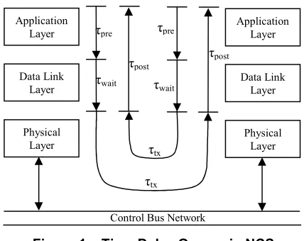
The important time delays in NCS occur when sensors, actuators, and controllers exchange data across the network. In an NCS, message transmission delay can be broken into two parts: device delay and network delay. A time diagram in Figure 1 shows time spent on sending a message from a source node to a destination node. Time delay includes the time delays at source and destination nodes and the transmission time. The time delay at source node includes the processing time, τpre, and the waiting time, τwait. The time delay at the destination node is the post-processing time, τpost. The network time delay, τtx, includes the total transmission time of the message and the propagation delay of the network. The total time delay equals the sum of the time delays τdelay=τpre+τwait+τtx+τpost.
The processing time at the source node is the time needed to acquire data from the external environment and encode it into the appreciate network data format. This time depends on the device software and hardware characteristics. In many cases, it may be assumed that the pre-processing time is constant or negligible. In fact, there may be noticeable differences in processing time characteristics between similar devices and these delays may be significant.
A message may spend time waiting in the queue at the sender’s buffer and could be blocked from transmitting by other messages on the network. Depending on the amount of data the source node must send and the traffic on the network, the waiting time may be significant. The main factors affecting waiting time may be protocol, message connection type and network traffic load.
The post-processing time at the destination node is the time taken to decode the network data into the physical data format and output to the external environment.
The transmission time is the most deterministic parameter in a network system. It only depends on the data rate, the message size and the distance between two nodes. The transmission time can be described as τtx=N×τbit+ τprop, where N is the message size in terms of bits, τbit the bit time, τprop the propagation time between any two devices. The propagation time is negligible in a small scale control network (100m or shorter) because of the high transmission speed (2×10⁸m/s).
2.2
Analysis Time Delay Effects in NCS
In a NCS, network is used to transmit data among control system devices. When sensors, actuators and controllers are interconnected by one common-bus network, all devices need to share the transmission medium, and the application signals are discretized. Hence, digital control approach is used for analysis of these types of systems. To guarantee the system stability and control performance, phase margin can be used.
Phase margin measures how far the closed-loop system is from stable/unstable conditions. It is the amount of extra phase shift that the system can tolerate before the closed-loop becomes unstable. It is the amount by which the phase shift of an open-loop system exceeds -180° when the gain equals one. For the system to be stable, the phase margin must be positive. The primary effect of time delay is additional phase-lag. It does not affect the magnitude frequency response curve. The typical effects of time delay are shown in Figure 2. The phase-lag caused by the time delay reduces the phase margin. If the phase margin becomes negative, the system becomes unstable.
)
(log
scale
ω
Amplitude (dB)
1
Gain Plot
[image:2.595.310.524.90.260.2]Phase (Degree)
Figure 2. Time Delay Effects in NCS
Application Layer
Data Link Layer
Physical Layer Application
Layer
Data Link Layer
Physical Layer
τpre τpre
τwait τ wait τpost
τpost
τtx
[image:2.595.311.509.396.544.2]τtx
Figure 1. Time Delay Occurs in NCS
Control Bus Network
)
(log
scale
ω
0 -90 -180 -270 -360
Phase Plot Without Delay Phase Plot With Delay Phase Plot
3
Missing Data and Make-up Work
When using an NCS, one must consider not only network-induced delays, but also data packet dropout. The messages to be transmitted can be lumped into one network packet (Single-packet Transmission). Due to the bandwidth and packet size constrains of the network, the measurements may be transferred using multiple network packets (Multiple-packet Transmission). Because of network access delays, the controller may be to receive all/parts/none of the packets by the time of control calculations. The network can be designed to re-transmit message for a limited time on the protocols with transmission-retry mechanism, but the packet are dropped after this time. For real-time feedback control data such as sensor measurements and calculated control signals, it may be advantageous to discard the old, un-transmitted message and transmit a new packet if it is become available. In this way, the controller always receives updated data for control. Normally, feedback-controlled plants can tolerate a certain amount of data loss.
We will consider a simple structure with just one controller and one process connected via network Figure 3. The information is exchanged using a network among control system components such as sensors, actuators, and controllers. The plant variable y(k) to be controlled is measured and the measurement is transmitted to the controller via the network. The controller compares it with a reference r(k), a desired response, and calculates the control output u(k) based on the error signal e(k). The controller output is transmitted to the plant to adjust the controlled variable. In the case of packet loss the prediction can makeup the data ŷ(k) to replace the lost packet y(k).
3.1
Plant Analysis Using Root Locus
In this study, we use Magnetic Levitation System (MLS), characterized by open-loop instability and non-linear dynamics, as the plant. This MLS suspends a hollow steel sphere with the aid of electro-magnetism inside an operating region. It can be modeled as:
) 1 5 . 30 / )( 1 5 . 30 / (
6 . 1 P
(
s
)
=
s + s −G
(1) The discrete-time transfer function GHP(z) of the plant model can be obtained using z-transform as follows) 1 )( 1 (
) ( 8 . 0
HP 1
2 1 1
1 2
)
z
(
G
− −− −
− −
+
=
z m z m
z z m
(2)
where m=e-30.5T+e30.5T-2, m1=e-30.5T, m2=e30.5T, and T is the sampling time.
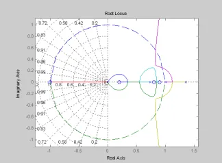
The root locus can be used to analyze the system behavior. The stability of the system may be determined from the locations of the closed-loop poles in the z-plane, or the roots of the characteristic equation. For all the root loci, there is a part inside the unit circle, i.e., a range of gain k can be found to assure all the close-loop poles inside the unit circle. The main idea of root locus method is to find the closed-loop response from the open-loop root locus plot.
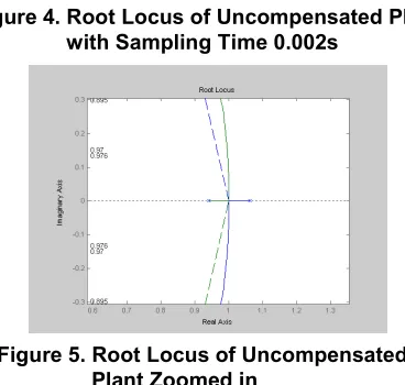
Using Matlab we get the root locus plot of the uncompensated plant shown as Figure 4. Figure 5 should be of the same root locus magnified a little so that the root locus around 1 on the real axis can be seen. In Matlab command window, using the user-defined function rlpoba, which returns the values of breakaway/breakin points of the root locus [17], we obtained the breakaway point at 1.0009 and the breakin point at -3.0009 on the real axis. Inspecting Figure 4 and Figure 5, only a small part of the root locus are inside the unit circle. At least one root is always outside the unit circle on a root loci which lies between the pole, 1.0629, and the zero, -1. It is necessary to reshape the root locus by adding the additional controller GC(z) to the open-loop transfer function.
3.2
Compensation with PID
nController
[image:3.595.322.521.145.520.2]We apply simplest PIDn controller, which has the structure of
Figure 5. Root Locus of Uncompensated Plant Zoomed in
[image:3.595.343.504.221.338.2]ŷ(k)
Figure 3. Networked Control System
_ +
Sensor Plant
Predict
y(k) u(k)
Controller r(k)
T
Network
e(k) Figure 4. Root Locus of Uncompensated Plant
[image:3.595.329.513.342.517.2] [image:3.595.63.267.348.421.2]1
1 n 1 n 2 2 1 1 0
1 C
(
)
G
−− − + − −
− + ⋅⋅ ⋅ + + +
=
z z q z q z q q
z
(3)The resulting difference equation is
)
1
(
...
)
2
(
)
1
(
)
(
q
1)
-u(k
u(k)
1 2
1 0
−
−
+
+
−
+
−
+
+
=
+
e
k
n
q
k
e
q
k
e
q
k
e
n
(4)
where u(k) is the output of controller, e(k), e(k-1), …, e(k-n-1) are the input errors.
Obviously, the controller is closely depending on the measurements or system errors.
With a PID3 controller, the open-loop transfer function of the system is given by:
) z 1 )( z 1 )( 1 (
) z )(
z ( 8 . 0 HP
C 1
2 1 1 1
4 4 3 3 2 2 -1 1 0 2 1
)
z
(
G
kG
− − −− − − −
−
− − −
+ + + + +
=
m m z
q z q z q z q q z km
(5)
The characteristic equation is given by:
0
)
z
(
G
kG
1
+
C HP=
(6)The placement of the zeros in the controller is a matter of trial and error. The problem using root locus method does not necessarily have a unique answer. The poles of this compensating work can be placed along the real axis between ±1. Three poles at origin force a fast response. A pole at -1 is a part of this PID3 controller. The additional zeros of the compensator will be placed inside the unit circle to pull the root locus further into the unit circle. For instance, we chose the roots 0.2, 0.5, 0.8, 0.9, for the polynomial, q0+q1z-1+q2z-2+q3z-3+q4z-4, which makes q0=1.0000, q1=-2.4000, q2=2.0100, q3=-0.6740, q4=0.0720. The root locus diagram plotted with Matlab is shown as
Figure 6. Figure 7 is a zoomed in diagram of Figure 6 around origin area. From the diagram, the braches of the root locus all have at least a part inside the unit circle. We can obtain the range of gain k to make all the close-loop roots are inside the unit circle that makes the system stable.
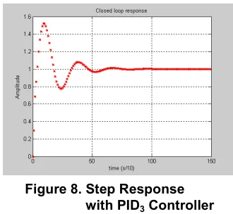
We may select a gain that will satisfy our design requirement to make the system stable. We can use Matlab command rlocfind to help. Command rlocfind returns selected poles on the root locus and the corresponding gain k. This value can be put into the system and the closed-loop response to a step input can be obtained. The step response of the system with PID3 is shown as Figure 8, in which sampling time T=0.002s, the closed-loop gain k=100.
From this plot as shown in Figure 8, we can see the system is stable.
3.3
Effect of Missing Data on System
Performance
If any measurement packets from sensor are dropped, a make-up work should be done to estimate the dropped data. When packet drops, we can use previous received packets to replace the lost packet. Consider e(k) is missing, and being updated with e(k-1), the controller transfer function takes the form of
1
4 4 3 3 2 2 1 1 0
1 ) ( C
(
)
G
−− − − −
−
+ + + +
=
z
z q z q z q z q q
[image:4.595.59.296.92.581.2]z
(7) [image:4.595.340.505.250.402.2]Figure 9. Step Response for e(k) Replaced with e(k-1)
Figure 8. Step Response with PID3 Controller
Figure 7. Root Locus with PID3
[image:4.595.87.255.429.593.2]Controller Zoomed in
[image:4.595.333.522.553.724.2]If we keep the same values of qi, i=0, 1, 2, 3, 4, as of the case without packet loss, the system becomes unstable. The system step responses are as shown in Figure 9.
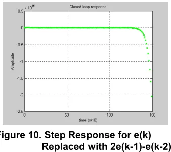
When packet drops, we can use linear interpolation methods. For updating e(k) with 2e(k-1)-e(k-2), we have the system transfer function:
1 4 4 3 3 2 0 2 1 0 1 1 ) ( ) 2 ( C
(
)
G
− − − − − − + + − + +=
z z q z q z q q z q qz
(8)where 2e(k-1)-e(k-2) is e(k-1) plus the difference between e(k-1) and e(k-2).
Similar as addressed as the case of simple data make-up method, if we keep the same values of qi, i=0, 1, 2, 3, 4, the system becomes unstable. The system step responses are as shown in Figure 10.
The missing packets, we can also use the polynomial method to do the make-up work. The polynomial is given by 0 1 2 2 1
1
x
a
x
...
a
x
a
a
y
vv v
v
+
+
+
+
=
−− −
−
(9)
For sequences e(k-1), e(k-2),…,e(k-v), we have:
− + − + −⋅⋅⋅ − = ⋅ ⋅ ⋅ ⋅ ⋅ ⋅ ⋅ ⋅ ⋅ ⋅ ⋅ ⋅ ⋅ ⋅ ⋅ ⋅⋅⋅ − − − − − − − − − ) ( ) 1 ( ) 2 ( ) 1 ( 1 1 1 1 1 1 2 2 2 2 1 3 3 3 3 1 0 1 2 1 2 2 1 2 2 1 2 2 1 2 2 1 v k e v k e v k e k e a a a a v v v v v v v v v v v v v (10)
With the solution of
⋅
⋅
⋅
=
− 0 1 2 1a
a
a
a
a
v ,We obtained polynomial of e(k-1), e(k-2), e(k-3) and e(k-4) to make up a datum to update e(k). For example, v=4, we can derivate values of ai, i=0, 1, 2, 3, in
0 1 2 2 3
3
x
a
x
a
x
a
a
y
=
+
+
+
. Then, we can compute y=e(k) for x=k, i.e. e(k)=4e(k-1)-6e(k-2)+4e(k-3)-e(k-4).We obtained the transfer function:
1 4 0 4 3 0 3 2 0 2 1 0 1 1 ) ( ) 4 ( ) 6 ( ) 4 ( C
(
)
G
− − − − − − − + + + − + +=
z z q q z q q z q q z q qz
(11)The system is unstable if qi, i=0, 1, 2, 3, 4, are the same as cases without packet drops. The system step responses are as shown in Figure 11.
Viewing the diagrams as shown in Figure 11, when packet drops some make-up methods can make the system instable if we keep the same PID3 controller parameters as without packet dropping. Some data make-up methods will degrade the system performance, but the system can still be stable. We can also see from the diagrams, the polynomial interpolation method has best system performance amongst the three methods. The more the interpolation points and the better approximation polynomial, the better system performance will be.
3.4
Controller Design
All these three methods can be written up in one formula as: 1 4 4 3 3 2 2 1 1 1 C
(
)
G
− − − − − − + + +=
z z p z p z p z pz
(12) [image:5.595.341.505.253.373.2]where pj, j=1, 2, 3, 4, are functions of qi, i=0, 1, 2 , 3, 4. The relationship is shown as Table 1.
Table 1. Relationship between pj and qi
Equations Parameters
Equation (7)
p1=q0+q1 p2=q2 p3=q3 p4=q4
Equation (8)
p1=2q0+q1 p2=q2-q0 p3=q3 p4=q4
Equation (11)
p1=4q0+q1 p2=q2-6q0 p3=4q0+q3 p4=q4-q0
Then we have the open-loop transfer function as:
) 1 )( 1 )( 1 ( ) )( ( 8 . 0 HP C 1 2 1 1 1 4 4 3 3 2 2 1 1 1 2
)
z
(
G
G
− − −− − − − − − − − − + + + +
=
z m z m z z p z p z p z p z z m (13) [image:5.595.88.257.264.414.2]Figure 11. Step Response by Polynomial Interpolation Method
[image:5.595.73.290.459.634.2]Using similar procedure in section 3.2, we chose the roots 0.2, 0.95, 0.95, for the polynomial
4 4 3 3 2 2 1 1
− −
−
−
+
+
+
z
p
z
p
z
p
z
p
which makes the system stable. Then we have p1=1.0000, p2=-2.1000, p3=1.2825, p4=-0.1805. The root locus diagram plotted with Matlab is shown as Figure 12. The system step response is shown as Figure 13, in which the sampling time T=0.002s, and the closed-loop gain k=75.
Then, we adjust qi, i=0, 1, 2, 3, 4, to keep the same pj, j=1, 2, 3, 4. For the case e(k) is updated with e(k-1), we adjust q0=-1.0000, q1=2.0000, q2=-2.1000, q3=1.2825, q4 =-0.1805, to get the same system step response as shown in Figure 13. Similarly, for e(k) updated with 2e(k-1)-e(k-2), we adjust q0=-1.0000, q1=-1.0000, q2=-1.1000, q3=1.2825, q4=-0.1805; for e(k) updated with polynomial
e(k)=4e(k-1)-6e(k-2)+4e(k-3)-e(k-4)
We adjust the parameters q0=1.0000, q1=-3.0000, q2=3.9000, q3=-2.7175, q4=0.8195, we can have the same result as shown in Figure 13.
The optimization result shows that as long as the PID3 controller parameters are adjusted to obtain a set of optimized parameters, better system performances can always been achieved. These methods can be expended to PIDn controller.
4
Conclusions
The time-delay and packet drop problems have been investigated in a PIDn NCS system over unreliable network links. First, we analyze the impact of time delay on control system performance, and conclude that the time delay will reduce system phase margin and gain margin, and degrade system stability. For packet drop and data missing problem, we investigates three data-making up techniques. We find that, the more the interpolation points and the better approximation polynomial, the better system performance will be. The polynomial interpolation method has best system performance amongst the three methods. Further study shows that the three data make-up methods can be modeled in one formula. The system performance only depends on the numerator polynomial coefficients of the formula. If the PIDn controller parameters are optimized to keep the same coefficients for this formula, the system performances will be the same for the three different data make-up methods.
5
References
[1] Michael S. Branichy, Stephen M. Phillips, and Wei Zhang, “Stability of Networked Control Systems: Explicit Analysis of Delay”, Proceedings of the American Control Conference, Chicago, Illinois, June 2000, pp. 2352-2357.
[2] Johan Nilsson, Bo Bernhardsson and Björn Wittenmark, “Stochastic Analysis and Control of Real-Time Systems with Random Time Delays”, Automatica, Vol. 34, No. 1, pp. 57-64, 1998.
[3] Johan Nilsson, “Real-Time Control Systems with Delays”, PhD Thesis, University of Toronto, Canada, 2003.
[4] Feng-Li Lian, James Moyne and Dawn Tilbury, “Analysis and Modeling of Networked Control Systems: MIMO Case with Multiple Time Delays”, Proceedings of the 2001 American Control Conference, Arlington, VA, USA, 25-27 June, 2001, Vol. 6, pp. 4306-4312.
[5] Mikael Pohjola, “PID Controller Design in Networked Control Systems”, M.S. thesis, Helsinki University of Technology, Greater Helsinki, Finish, January 2006.
[6] Luca Schenato, “Kalman Filtering for Networked Control Systems with Random Delay and Packet Loss”, 17th International Symposium on Mathematical Theory of Networks and Systems (MTNS'06), Kyoto, Japan, July 2006.
[image:6.595.92.254.215.334.2][7] Luca Schenato, “To zero or to hold control inputs in lossy networked control systems?”, European Control Conference (ECC'07), Kos, Greece, July 2007.
Figure 13. Step Response for e(k) Missing
[image:6.595.88.257.373.526.2][8] Luca Schenato, Bruno Sinopoli, Massimo Franceschetti, Kameshwar Poolla, and S. Shankar Sastry “Foundations of Control and Estimation Over Lossy Networks”, Proceedings of the IEEE, Vol.95, No. 1, January 2007, pp. 163-187.
[9] Luca Schenato, “Optimal estimation in networked control systems subject to random delay and packet loss”, Proceedings of the 45th IEEE Conference on Decision & Control, San Diego, CA, USA, December 13-15, 2006, pp5615-5620.
[10] M. Sahebsara, T. Chen and S. L. Shah, “Optimal H2 filtering with random sensor delay, multiple packet dropout and uncertain observations”, International Journal of Control, Vol. 80, No. 2, February 2007, pp. 292–301.
[11] Qiang Ling and Michael D Lemmon, “Soft Real-time Scheduling of Networked Control Systems with Dropouts Governed by a Markov Chain”, Proceedings of American Control Conference, 4-6 June 2003, Vol. 6, pp. 4845-4850.
[12] Vijay Gupta, Demetri Spanos, Babak Hassibi and Richard M Murray, “On LQG Control Across a Stochastic Packet-Dropping Link”, 2005 American Control Conference, Portland, OR, USA , 8-10 June, 2005, pp. 360-365.
[13] Peter J. Seiler, “Coordinated Control of Unmanned Aerial Vehicles”, Ph.D thesis, University of California, Berkeley, 2001.
[14] Christoforos N. Hdjicostiss and Rouzbeh Touri, “Feedback Control Utilizing Packet Dropping Network Links”, Proceedings of the 41st IEEE Conference on Decision and Control (invited), Las Vegas, NV, USA, 2002, Vol. 2, pp. 1205-1210.
[15] Qiang Ling and Michael D. Lemmon, “Optimal Dropout Compensation in Networked control Systems”, Proceedings of the 42nd IEEE Conference on Decision and Control, Hawaii, USA, 9-12 Dec. 2003, pp. 670-675.
[16] Oscar Flärdh, Karl H. Johansson and Mikael Johansson, “A New Feedback Control Mechanism for Error Correction in Packet-Switched Networks”, Proceedings of the 44th IEEE Conference on Decision and Control, and the European Control Conference 2005, Seville, Spain, 12-15 December, 2005, pp. 488-493.