Rochester Institute of Technology
RIT Scholar Works
Theses
10-29-2018
A Transparent Square Root Algorithm to Beat
Brute Force for Sufficiently Large Primes of the
Form p = 4n + 1
Michael R. Spink
Follow this and additional works at:https://scholarworks.rit.edu/theses
This Thesis is brought to you for free and open access by RIT Scholar Works. It has been accepted for inclusion in Theses by an authorized administrator of RIT Scholar Works. For more information, please [email protected].
Recommended Citation
ROCHESTER INSTITUTE OF TECHNOLOGY College of Science
School of Mathematical Sciences
A Transparent Square Root Algorithm to Beat Brute
Force for Sufficiently Large Primes of the Form
p
= 4
n
+ 1
by
Michael R. Spink
October 29, 2018
Thesis submitted in partial fulfillment of the requirements for the degree of
MASTER OF SCIENCE
in
1
Committee Signature Page
Dr. Manuel Lopez Date
School of Mathematical Sciences, Rochester Institute of Technology Thesis Advisor
Dr. Anurag Agarwal Date
School of Mathematical Sciences, Rochester Institute of Technology Committee Member
Dr. James Marengo Date
School of Mathematical Sciences, Rochester Institute of Technology Committee Member
Dr. Matthew Hoffman Date
2
Abstract
Finding square roots in the modular integers is a well known problem that is the basis for many
modern cryptosystems. For primes of the formp = 4n+ 3, given C ∈ Z×
p, finding solutions to
x2 ≡ C (mod p) is deterministic. For primes of the form p = 4n+ 1, no known deterministic computation exists for determiningx given C. Tonelli (later improved by Shanks,) Cipolla, and Pocklington, among others, found sophisticated algorithms to perform this task. Brute force is a
transparent approach, but offers no insights into the problem. In this thesis, we produce a
trans-parent approach to this problem, visualized using a model built on Symplectic Geometry. One of
the insights from viewing the problem in this way is a conjecture on the distribution of quadratic
residues, which we exploit in our algorithm. Even though the conjecture is not essential to the
workings of the algorithm, it gives it an edge over brute force for large enough primes. Finally, we
3
Acknowledgements
Firstly, I would like to thank my thesis advisor, Dr. Manuel Lopez for being by my side
mathemat-ically, time wise, and just being someone to talk to about PiRIT or whatever else is the topic of the
day. Without your help there is no way this thesis would be done. I would also like to thank Dr.
Anurag Agarwal and Dr. Jim Marengo for being co-advisers on this thesis and providing me with
an endless number of Putnam problems to whittle away at when wanting to get away from actual
coursework.
Secondly, I would also like to thank the Director of the MS program, Dr. Matthew Hoffman, the
heads of the School of Mathematical Sciences, Dr. Tamas Wiandt and Dr. Matthew Coppenbarger,
the Dean of the College of Science, Dr. Sophia Maggelakis, and the staff members of the School
of Mathematical Sciences, Tina Williams, Ginny Gross, Corinne Teravainen, and Anna Fiorucci
for their support while I was working on this thesis and my work as a whole at RIT. I would also
like to thank Dr. David Barth-Hart and Kesavan Kushalnagar for their support and comments that
helped direct my efforts in various ways.
Most importantly, I want to thank my parents, my siblings, and my family as a whole for always
being there for me. I would also like to thank my friends at home and at RIT, everyone in PiRIT,
and everyone I have forgotten or haven’t found a bucket to dump you in for your support and for
helping me even in the worst of my days.
Contents
1 Committee Signature Page i
2 Abstract ii
3 Acknowledgements iii
4 Introduction/Preliminaries 1
4.1 The square root problem and number theory . . . 1
4.2 Relevant Symplectic Geometry . . . 7
5 Previous Work 11 6 Geometrical solutions to the square root problem 15 6.1 Transforming the problem into symplectic geometry . . . 15
6.2 UsingΩto solve for the square root . . . 19
6.3 The Front-Loading Conjecture . . . 23
7 An Algorithm to find the square root 27 7.1 The Preprocessing steps . . . 28
7.2 Crux of the Algorithm: The Repeated Multiplication . . . 32
7.3 Comparing our algorithm to Brute Force . . . 35
7.4 Improving the Design of the Algorithm . . . 40
7.5 Simple working examples of repeated multiplication . . . 44
8 Future work 48
9 Conclusion 49
10 Appendix 1: Code 50
List of Tables
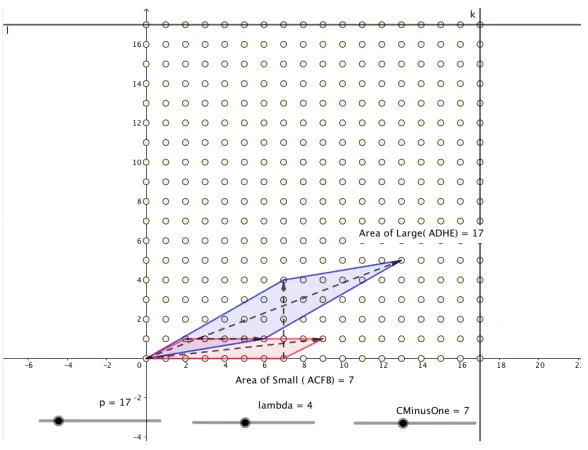
1 Table of determinants usingΩmod 13 . . . 21
2 Table of determinants usingΩmod 17 . . . 21
3 Howρandξis computed for small4n+ 1primes . . . 24
4 How the cases of preprocessing partitionZ×p . . . 29
5 Comparing runtimes for1 (mod 8)primes . . . 36
6 Comparing runtimes of other primes . . . 36
7 Comparing iterations for various4n+ 1primes . . . 38
8 The runtime effects of just using Euler’s Criterion . . . 40
9 The runtime effects of just using a Collatz approach to preprocessing . . . 41
List of Figures
1 Commutivity diagram for our manifold. . . 172 Illustration that√8≡5 (mod 17) . . . 20
3 A graph ofQR101. . . 23
4 Howρis affected aspincreases . . . 25
5 Howξis affected aspincreases . . . 26
6 Howξaffectsρ . . . 26
7 The general flow of the algorithm . . . 28
8 Running 10,000 random trials forp= 73529to see runtime . . . 35
9 The most time consuming steps of the algorithm . . . 37
10 Running 10,000 random trials forp= 73529to see iteration count . . . 38
[image:7.612.91.544.361.604.2]List of Symbols and Notation
p Prime number, usually of formp= 4n+ 1
Z×p The group of units modp, i.e{1,2,· · · , p−2, p−1}
C Potential Quadratic Residue to find the square root of
x Solution to the Square Root Problem, if it exists
λ Shifted Solution to the Square Root Problem, if it exists
QRp, N Rp Sets of Quadratic Resides and Quadratic Nonresidues, respectively
|G| cardinality of set or groupG.
ord(m) order of elementminZ×p
< α > subgroup generated by elementα∈G
g Primitive Root forZ×p
a, b Integers in the decomposition ofp=a2+b2
V Vector space in which a symplectic manifold is set
Ω Two form for manifold
˜
Ω Dual mapping forΩ
π Symplectomorphism to create our symplectic manifold
R Table of Determinants for modp.
“Quadrant” Forp= 4n+ 1, each of the interval of integers[1, n][n+ 1,2n][2n+ 1,3n][3n+ 1,4n]
ρ Ratio between Quadratic Residues in Quadrant II to those in Quadrant I
ξ Difference between Quadratic Residues in Quadrant II to those in Quadrant I
Q, s Coefficients in decomposition ofp−1 = Q∗2s
A Set of integersα1 inZ×p such thatα
Q
1 ≡1 (mod p)
B Set of integersα2 inZ×p such thatα
Q
2 ≡ −1 (mod p)
yi Perfect integer squares to use in algorithm
χ Representation of the current value being looked at in the algorithm
Ψ Representation of the integer multiple to invert in the algorithm.
κ Boolean representation of the need to compute√−1in the algorithm.
4
Introduction/Preliminaries
For this thesis we assume a working knowledge of discrete math and basic matrix operations. The
rest of the groundwork for this thesis will be laid out in this section.
4.1
The square root problem and number theory
We begin by defining the problem that we are examining in this thesis.
Definition 1. Square root Problem [16]
ConsiderZ×p for an odd prime integerp. Solutions to the modular equation
x2 ≡C (mod p) (1)
forxwherex, C ∈Z×
p andC is known, solves the square root problem modp.
We can equivalently write this as
x≡√C (mod p) (2)
to emphasize the name of the problem.
We also now lay out some basic facts that we will be referencing throughout this thesis.
Definition 2. Quadratic Residue modp[6, pp. 98]
The variable C in the square root problem is known as a quadratic residue mod p whenever a solution exists.
We will sometimes call these QRs for short.
Definition 3. Quadratic Non Residues modp.[6, pp. 98].
Values inZ×p that are not quadratic residues mod p are known as non-residues modp.
We sometimes call these NRs for short. We can also use the following shorthand when referring
to these values as a set. As will be seen in Theorem 3, only the QR’s form a group, due to a lack
Definition 4. Sets of Reciprocity [1]
Letpbe prime. Then we define the following sets:
QRp ={y ∈Z×p|∃x∈Z
×
p, x
2 ≡y (mod p)}
(3)
N Rp ={y ∈Z×p|∀x∈Z
×
p, x
2 6≡y (mod p)}
(4)
We do know the cardinality of these sets.
Theorem 1. Cardinality of the sets of Reciprocity [5, pp 121].
Letpbe prime. Then
|QRp|=|N Rp|=
p−1
2 (5)
Proof. The well-known Lagrange’s Theorem (see Theorem 2) implies x2 ≡ C (mod p) has at most two solutions. Ifx0 ∈Z×p is such thatx20 ≡C (mod p), then(−x0)2 ≡C (mod p). Either
p= 2and thusZ×2 ={1}orpis odd, thusx0 6=−x0, and it follows that ifx2 ≡C (mod p)has a
solution, then it has exactly two solutions.
Put another way, we can establish the function f : Z×p → Zp× such thatf(x) ≡ x2 (mod p)
and note thatf is a two-to-one function. The ending of this proof establishes the following result
Lemma 1. Number of solutions to the square root problem
Letpbe prime and letx2 ≡ C (mod p)have a solution. Thenx2 ≡ C (mod p)has exactly two
solutions.
From this, we know that the sets of Reciprocity partitionZ×p.
Corollary 1. Partition ofZ×p by sets of Reciprocity.
Letpbe prime. ThenN RpandQRp partitionZ×p
Proof. Clearly by Definition 4 these two sets are disjoint and are subsets ofZ×p. Now we note that
|Zp×| =φ(p) = p−1. Consider N Rp S
QRp. Since these two sets have p
−1
2 elements, the entire
union must havep−1elements. This proves the corollary.
Definition 5. Order of an element in a group [9, pp. 105]
Let G be a group and g ∈ G over multiplication with identitye. Then the order ofg, denoted
ord(g), is the least integerksuch that
gk =e. (6)
Whenk =|G|in the above definition, we have a special element of a group. We will be using these quite a bit in this thesis.
Definition 6. Primitive root/Generator modp[6, pp. 79].
Letpbe prime, and Gbe a group. Theng ∈ Gis a primitive root if powers ofg generate every element inG.
We denote by< b >the group of elements generated byb∈Z×
p [6, pp. 79].We state Lagrange’s
Theorem here, bridging the gap between the order of an element and the order of a group.
Theorem 2. Lagrange’s Theorem [9, pp. 129]
LetGbe a group, andg ∈G. Thenord(g)| |G|
Proof. See [9, pp. 129]
Returning to the discussion of residues, a property of QR’s/NR’s that we will need is as follows:
Theorem 3. Product of Residues [5, pp 124]
Letpbe prime and letw, x∈QRp andy, z ∈N Rp. Then:
wx∈QRp, wy∈N Rp, yz ∈QRp (7)
Proof. Letg be a primitive root modp. ThenC ∈ QRp iff C ≡ g2k (mod p)and C ∈ N Rp iff
C ≡ g2l+1, withk, l ∈
N. Then the conclusion follows the parity properties of the addition of
natural numbers.
We can also now determine that the Quadratic residues form a group.
Corollary 2. Existence of the Group of Quadratic Residues
Proof. Theorem 3 gives us closure over multiplication. Due to the fact that this is over standard
multiplication, 1will be the identity of the group. Trivially, 1 ∈ QRp. As 1 ∈ QRp and due to
Theorem 3, all QR’sm have inverses m−1 ∈ QR
p. Lastly, we are granted associativity, as it is
inherited from the larger group,Z×p.
We can quickly determine ifais a quadratic residue by Euler’s Criterion.
Theorem 4. Euler’s Criterion [6, pp. 68-69]
Let p be a prime, andm∈Z×
p. m∈QRp iff
mp−21 ≡1 (mod p) (8)
From here, it is easy to find the quadratic character of specific elements inZ×p. For Example:
Corollary 3. Quadratic Character of−1[5, pp. 126] Letpbe an odd prime. Then−1∈QRp iffp= 4n+ 1
From this and the closure of QRs, we have the following result.
Corollary 4. Quadratic residue property of4n+ 1primes Letp= 4n+ 1be prime, and leta∈Z×
p. a∈QRp iff−a∈QRp
Similarly, ifp= 4n+ 3,a∈QRp iff−a∈N Rp
Alternatively, one may use the Law of Quadratic Reciprocity, the properties of the Legendre
Symbol, and Gauss’ Lemma [6, pp. 68-69,101-103] to determine the quadratic character of an
integerm ∈ Z×
p. Often, however, this involves knowing the prime factorization of m, which is a
challenging task. Further, finding the square root ofm, if there is one, is more challenging. This is what we set out to do.
Now, we discuss some known results for specific primes to aid in finding the square root. The set of
Theorem 5. Finding the square root for4n+ 3primes [8].
Letp≡3 (mod 4),be prime. The square root,x, of quadratic residueCis:
x≡ ±Cp+14 (mod p) (9)
It is worth noting that eitherC or−C is a quadratic residue, but not both, in accordance with Corollary 4
There are similar formulas for increasingly restrictive properties on primes of the formp= 4n+ 1, but there is no similarly simple formula in general. Trivially, one could square every value of x
from 1 to p−21, but this is inefficient for large primes. This is the brute-force method for finding the solution to the square root problem.
Thus, to do better than brute force to solve square root problems, we exploit properties of primes
of the formp= 4n+ 1. The two properties that we will be using of these often called Pythagorean Primes are as follows:
Theorem 6. Pythagorean property of4n+ 1primes [14]
Letp= 4n+1be prime. Then we can writepuniquely as the sum of two squares over the integers, that is
p=a2+b2 (10)
This is called the Pythagorean Property of4n+ 1primes because it resembles the Pythagorean Theorem.Fermat was the first to conjecture about this, and Euler proved it.
Don Zagier came up with a method to find this decomposition ofp, which we have implemented in Section 10. We call this the Zagier Method henceforth. Shailesh A Shirali expanded on this
idea, and developed an algorithm to constructively findp=a2+b2. Biman Bagchi proved that the
algorithm always terminates, yielding the answer. [14]
Corollary 4 indicates that−1 ∈QRp forp = 4n+ 1. Now, as a result of Theorem 6, we will
Lemma 2. Finding√−1 (mod p)
Given primepand integersa, bsuch thatp=a2+b2. Then
√
−1≡ab−1 (mod p) (11)
and
√
−1≡a−1b (mod p) (12)
Proof. Modulo p, we have
a2+b2 ≡0 → a2 ≡ −b2 (13)
Considerab−1When we square this, we get
(ab−1)2 ≡a2(b2)−1 ≡ −b2(b2)−1 ≡ −1 (14)
The proof fora−1bis similar.
Ideally, the general solution the square root problem would come from a solution to the discrete
log problem. Since this is unlikely due to the “difficult” nature of the problem - it is in the
com-plexity class NP, among other classes, while the decision portion of the problem is indeed in class
P, due to the ease of using Euler’s Criterion [6, pp. 68-69]. We are left with a brute force approach
to find the numerical answer to the square root problem, or a less than transparent approach like
Tonelli-Shanks’, Cipolla’s, or Pocklington’s Algorithms. We say this as these methods rely on the
Discrete Logarithm (Tonelli-Shanks) or Quadratic extensions (the other two) [2]. We discuss these
three algorithms in more detail in Section 5.
4.2
Relevant Symplectic Geometry
For our problem, we need to build a Symplectic Manifold. We pull everything in this section and
follow the conventions of Silva [3] unless otherwise stated. Our geometry will not be couched in
differential notation. Darboux’s Theorem will account for the difference in construction, avoiding
any discrepancy. To this end, we note only what we see as paramount in creating a symplectic
manifold.
We start with a given vector space V. In our case, V will be R2. A symplectic manifold is based on a symplectic vector space, which is based on a skew symmetric bilinear map. We we call
this mapΩ :V ×V →R
Definition 7. Bilinear Map [3]
Consider mapΓ :X×Y →Z,and letΓx0 = Γ(x0, y), wherex0is fixed andΓy0 = Γ(x, y0)where
y0is fixed.Γis bilinear ifΓx0 is linear for everyx0 ∈X andΓy0 is linear for everyy0 ∈Y.
Definition 8. Skew Symmetric Map [3]
MapΓ :X×X →Z is skew symmetric if
Γ(u, v) =−Γ(v, u) ∀u, v ∈X×X (15)
In our case,Ωwill turn out to be
Ω(u, v) =det
−~u− −~v−
=~u T
0 1
−1 0
~v (16)
and we see that
Ω( a b , c d ) = a b 0 1
−1 0 c d = a b d −c
=ad−bc=det a b c d (17)
Further, note that this map is linear by the properties of determinant and matrices, so ourΩwill be bilinear. We will reference this later.
Definition 9. Dual Map [3]
LetΩ :V ×V →Rbe a skew symmetric bilinear map. ThenΩ˜, called a dual map, is the mapping fromV into its dual, denotedV∗. Further, this map is
˜
Ω(~u) = Ω(~u, )∈Hom(V,R) (18)
Since Ω’s co domain isR, the dual ofV are the functionals that map into R. Following our
example, one could defineΩ˜ as follows.
˜
Ω(~u) = det
u1 u2
x y
(19)
We now put this map into the vector space properly.
Definition 10. Symplectic Map/ Symplectic Linear Structure/Symplectic Vector Space [3]
LetΓ :V ×V →Rbe a skew symmetric bilinear map. Γis symplectic, ifΓ :˜ V →V∗is bijective. We call(Ω, V)a symplectic vector space, andΩa symplectic linear structure onV.
This does bring up a property of Symplectic Vector Spaces that will confirm our use ofV =R2 Theorem 7. Even degree Manfolds in Symplectic Linear Structures [3]
LetΩ :V ×V →Rbe a symplectic linear structure onV. Thendim(V)is even.
We can relate two symplectic vector spaces, or a symplectic vector space with itself with a
Symplectomorphism.
Definition 11. Symplectomorphism [3]
Let(V,Ω)and(V0,Ω0)be symplectic vector spaces in vector spacesV, V0. These two spaces are symplectomorphic if there exists a linear mappingπ :V →V0, the symplectomorphism, such that
Definition 12. Manifold [18]
A ManifoldM is a topological space that is locally Euclidean at every point in the space.
This means that for manifold M and every x ∈ M there is an open neighborhood U and a bijective homeomorphismh:U →V where V is a neighborhood of the origin inR
We want the manifold to maintain the properties of the original symplectic vector space .
Rel-evantly to us, we want to ensure that the manifold maintains the local topology of R2 as we are
usingV =R2.
Definition 13. Symplectic Manifold [3]
A Manifold M in space V, symplectically paired with 2-form Ω is a Symplectic Manifold if at every point p on the manifold, there corresponds a tangental plane, denoted TpM, and on this
tangental plane the mapΩp is a symplectic linear structure inV. We denote the manifold(M,Ω)
For our purposes, we want all of theseΩp = Ωto carry out the geometric interpretation of the
square root problem that we will create in Section 6.1. Darboux’s Theorem will allow us to view
the answer to one square root problem in relation to other square root problems for the same prime.
We present this theorem without differential notation.
Theorem 8. Darboux’s Theorem [3]
Let(M2n,Ω)be a symplectic manifold. For every point in the manifold, there is an open
neigh-borhood diffeomorphic to an open neighneigh-borhood of the origin inR2nand every pair of points on the manifold have diffeomorphic open neighborhoods.
The standard differential 2-form onR2nis
Ω0 = n X
j=1
dxj ∧dyj[12] (21)
and Darboux’s Theorem implies that for every point on the manifold (M2n,Ω), there exists a coordinate chartφsuch that
φ∗Ω0 = Ω. (22)
This theorem implies that every point on the manifold behaves just like every other point on
the manifold. This gives validity to Brute Force being used as an approach to the answer the
square root problem. At some points, namely those corresponding to whereCis a perfect integer square, the answer to the square root problem is readily available by arithmetic. However, this is a
relatively few number of points compared to the entirety of the torus. Thus, our approach is to go
point to point to gather enough global information to be able to trace back from one of these points
to the solution of our given square root problem. As we will see, the important question is what
5
Previous Work
In this section, we focus mainly on the history on the square root problem and relevant related
topics, instead of focusing on symplectic geometry. We used this geometry as it is common to
present the addition and multiplication tables for Zp as embedded in a torus. Further, the
com-panion matrix that we will use to translate the square root problem into this context requires us
to solvedet(A−λI), and laterdet(A+λI),provides us with a natural skew symmetric 2-form, which segues nicely into using this geometry. More knowledge about symplectic geometry can be
found in [3].
Let us return to the square root problem, which falls into a well developed area of number theory
known as quadratic reciprocity. Many of the results, however, strictly address whether of notCis a quadratic residue modp. This is how the Legendre and Jacobi symbols are defined [5, pp. 123]. For example:
Theorem 9. [5, pp. 128] Quadratic Character of 2
2is a Quadratic residue modpiffp= 8n+ 1orp= 8n+ 7.
The Law of Quadratic Reciprocity is also extremely useful in this regard.
Theorem 10. The Law of Quadratic reciprocity [5, pp. 130-131].
Letpandqbe distinct odd primes. Then
p q
q p
= (−1)(p−1)(4q−1) (23)
where
p q
=
1, p∈QRq
−1, otherwise
(24)
A considerable amount of work deals with the distribution of the quadratic residues as a whole.
Theorem 11. Small Consecutive QR result [17]
Letp≥11be prime. ThenZ×p has aq∈QRp >0such thatq+ 1 ∈QRp
Walum extends from just QR’s to kth power residues [17]. Further, for a prime p, there are
known formulas for the number of sequences of QR, followed by QR, sequences of QR, followed
by NR, sequences of NR followed by QR, and lastly, sequences of NR followed by NR, all
ap-proximately p4 [7]. Note that these cover the entirety of Z×p. There are also upper bounds found by Davenport for the number of sequences of QR, QR, QRandN R, N R, N R[7]. Finally, Per-alta cites Hudson for showing that the sequences ofQR, QR, N R, QR andQR, N R, QR, QRis nonzero for large primes [7]. Peralta worked to try to generalize these results [7].
Another body of work is into finding the least NR modp. Trivially the least QR modpis 1. Gauss in 1798 bounded the least NR by the following:
Theorem 12. Gauss’ upper bound for the least Nonresidue modulop. [7]
Letp= 8n+ 1be prime. Then the least nonresidue modpis less than or equal to2√p+ 1
However, this bound can be improved. Peralta cites Burgess for one such bound [7]. It is
pos-sible that the bound is 3(ln2p)2, however, this is dependent on the Generalized Reimann Hypothesis
[10].
There are three well publicized algorithms that aid us in solving the square root problem. The first
relies on the discrete log problem, known as the Tonelli-Shanks Algorithm [2], and the second two
rely on implicit quadratic extensions, known as Cipolla’s Algorithm and Pocklington’s Algorithm
[2]. We begin with the first of these, as it is the most well known. Tonelli-shanks relies on finding
anisuch that for an integertsuch that
t(2i) ≡1 (mod p)[15] (25)
In trying to solve Equation 1, thistis initalized toxQ (mod p),if we decompose p-1 as such:
Often, however, this initialization is indeed 1, and we can easily find the square root. Indeed,
Turner proves that this initialization immediately works in 23 of cases [16]. This relies on a proof
thatQmany elements satisfy
xQ ≡1 (mod p) (27)
for 4n+1 primes. Turner presents this proof in a probabilistic sense [16]. We will expand on this
with an alternative proof in Section 7.1. Further, [15] presents the runtime of this algorithm as an
argument in terms of the amount of multiplications. This will not be our way to assess runtime due
to the difficulty to arithmetically determine how long the algorithm will run. See Section 7.4 for
more information. Note however, the fact that finding thisican be difficult to compute by hand, as well as computing large powers ofx. Further, there are primes of specific forms that Tonelli-Shanks can be considerably slower, This is where we want to improve on this approach.
Cipolla in our view further lessens this transparency. In his attempt to solve Equation 1 do so, it
finds atsuch that
t2−a∈N Rp (28)
(ort2−a≡0 (mod p)), and after doing so, performing arithmetic to find the square root [15]. This approach loses a few things: the first is decidability. A precondition for Cipolla is thatx ∈ QRp.
The second is that it appears that there is no good strategy to picking t other than brute force and repeatedly computing the Legendre Symbol [15]. We hope to fix both of these things with
our algorithm in Section 7 Once again, [15] computes the runtime of this algorithm in terms of
modular multiplication.
Lastly, we touch on Pocklington’s algorithm. Pocklington focuses mainly on primes of the form
Theorem 13. Solution to the square root problem for8n+ 5primes [8] Letp= 8n+ 5be prime. Then ifC2n+1 ≡1 (mod p),
x≡ ±Cn+1 (mod p) (29)
Otherwise
x≡ (4C)
n+1
2 or
p+ (4C)n+1
2 (30)
depending on the parity of(4C)n+1
If p = 4n+ 3, Pocklington uses Theorem 9. So ifp = 8n+ 1, Pocklington finds constants
α1, β1 such that
α21+Cβ12 ∈N Rp[8] (31)
From there, Pocklington iterates on a two recurrence relations forα, β:
αn=
(α1+β1
√
−C)n+ (α 1−β1
√ −C)n
2 (32)
βn=
(α1+β1
√
−C)n−(α 1 −β1
√ −C)n
2√−C (33)
and performs some arithmetic onceαk ≡0. We find that this is further removed from Cipolla
and has the same problems that Cipolla did: decidability and transparency. The recurrence relations
indeed look daunting at a glance. However, this does give us a simple way to handle some of the
4n+ 1primes [8].
There have been other algorithms to find the square root. For example, in [13] uses ideas from
Elliptic curves to find an algorithm that runs inO(log9p), which is faster than brute force, and [11]
shows that methods can be derived from continued fractions. We do not emphasize Elliptic curves
here, which are outside the purview of knowledge that we view as “basic” relative to this problem,
furthering this issue of transparency.
We now begin deriving our algorithm from ideas that will help us understand the difficulty of
6
Geometrical solutions to the square root problem
In this section, we build a useful symplectic manifold that will allow us to look at the square root
problem in a non number theoretic way. The Ω in this manifold is then used to attempt to find a robust solution to the square root problem. Our approach is to gather global information on
the manifold help solve Equation 1, rather than the indiscriminate approach to the manifold used
by brute force. Our algorithm, discussed in Section 7, will benefit if a conjecture we discover
from looking at the manifold in this manner is true. We call this conjecture the Front-Loading
Conjecture. As will be seen, our algorithm will terminate successfully regardless of truth of the
conjecture.
6.1
Transforming the problem into symplectic geometry
Letpbe an odd prime and consider Equation 1: Consider shifting the problem by simply letting
x=λ−1:
(λ−1)2 ≡C (mod p) (34)
This expands to
λ2−2λ−C+ 1 =λ(λ−2)−(C−1)≡0 (mod p) (35)
so a companion matrixAfor this polynomial is
A=
2 C−1 1 0
(36)
Note however how the characteristic and minimal polynomials of this is the same as the expanded
To build this manifold, we begin with a smooth vector space,V =R2.Note thatdim(
R2) = 2,
which satisfies Theorem 7. Keep in mind that we will be using the integer lattice over this space in
due time. Our basis sets will be as follows:
{ui}= 1 0
∈V
(37)
{vi}= 0 1
∈V
(38)
We now build our bilinear map as in Equation 16.
Ω(~u, ~v) =det
−~u− −~v−
. (39)
As shown in Equation 17, this choice of Ω is skew symmetric. Based on the properties of the determinant, thisΩis bilinear, or more simply, linear in R. Further, note how the output ofΩis real valued by the definition of the matrix determinant. Now, fix
~ u= u1 u2 (40)
Then to keepΩ˜ similar to that ofΩ, we define
˜
Ω(~u) = det
u1 u2
x y
(41)
where x and y will be determined when something is plugged into this determinant function. Note
For example, let~u=
1 2
, then
˜
Ω(~u) = det
1 2
x y
(42)
and
˜ Ω(~u)[
1 3
] = det
1 2 1 3
= 1 ∈R (43)
We denote the input of Ω˜ in square brackets. We know that this output is bijectively related to the choice of xandy. This means that(V,Ω)is a symplectic vector space. Now, we just need a manifold that has R2’s smoothness. To do this, we will use a symplectomorphism. LetV0 = V.
Considerπ :V ×V →V0×V0
π(a, b) = π(c, d) if p|(a−c) and p|(b−c) (44)
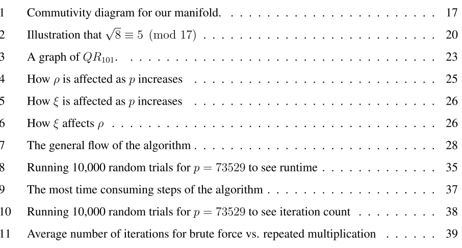
This creates an equivalence relationR onV ×V. LetΩ0 = Ωon these equivalence classes. We have gone fromV ×V toV0×V0toR.We can also illustrate this (and other symplectomorphisms) by the commutivity diagram in Figure 1.
R
V ×V
V0×V0
Π
Ω
0
on the equivalency
classes inV0×V0
[image:25.612.220.394.478.620.2]Ω
In essence, we are takingV and creating a cylinder out of it in “both” directions. Applied to a specific prime, this will turn into a representation ofR, or in terms of the integer lattice,Zp. This
torus will be the manifold that we will be working on. This is also the classical geometric picture
of the “donut” torus, yet made out of the real plane. This torus, combined with Ω, will be our symplectic manifold. Since this manifold maintains the properties of its underlying vector space,
this torus remains smooth. Thus, tangential planes exist at all points on this plane. Thus, This
manifold is symplectic. Note that we only care about the integer lattice on the torus. If there exists
a tangental plane at all real points on the torus, then clearly there is a tangental plane at every point
on the integer lattice on the torus.
Now that we have our torus and have shifted our problem, we look at what steps to take in our
attempts to solve the square root problem. We can change the primep to determine the specific manifold (and the points that are in equivalence classes), the value of C (the specific problem to
solve), and the potential solution to the problem,λ. For us, fixpto fix the specific manifold to work with. This leaves us with(C, λ)as points on our torus. Pick an arbitrary point on the torus, and call it the origin. Let theCaxis rotate counterclockwise around the torus from the origin. Since C are the problem to solve, C will range from1top−1Let theλaxis rotate around the “center” of the torus. Since xand−xare both solutions if one is, λ will range from 1 to p−21 −1.With this in mind, we have all possibilities for all of the square root problems. Those that fit certain criteria
6.2
Using
Ω
to solve for the square root
We will be finding the square root through a few related ideas here. First, we will be using Ω
directly to find if a solution is correct. We then holistically look at the entire torus in this lens to
improve on the brute force method.
Let A =
2 C−1 1 0
as described above. If we fix C and let it be a quadratic resiude, we
want to find wheredet(A−λI) ≡ 0 (mod p). That is, this determinant is a multiple ofp. For example, mod 13, say we want to find the square root of 3. ThusA=
2 2 1 0
Consider the matrix
A=
2−5 2 1 0−5
. The determinant of this matrix is 13, which is a multiple of 13. Since this
A−λI has been shifted at the outset of the problem (see equation 34), we have thatx+ 1 = 5, so
x= 4. Indeed,42 ≡3 (mod 13). Notice how this also works if you look forλ = 10, orx= 9.
To make this problem easy to compute by hand, we can convert the determinant into an similar
problem about finding the area of the parallelogram between the vectors of the columns of A. Begin
with A, so that the parallelogram in question is bounded between
2 1 and C−1
0
.Shift the
first of these vectors to the right by 1 at each iteration, and the second of these vectors up by 1 at
each iteration. We are now shifting the vectors in question up and to the right. Due to this shift,
we are looking atdet(A+λI) ≡ 0 (mod p)instead of the traditionaldet(A−λI) ≡ 0. This is valid to due the fact that we are working in the modular integers. We do this for the convenience
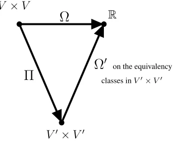
of arithmetic and to keep the picture in Quadrant I of our vector space,R2. Due to this shift, we similarly shift our solution tox=λ+ 1This may make the square root easy to identify, however, this is still infeasible to use for large primes, as one would still have to scan though all possible
areas to find the one that works. Though, perhaps the use of Pick’s Theorem would make things
easier to compute by hand. We can animate this in Geogebra. Figure 2 illustrates that √8 = 5 (mod 17). We identify λ = 4, so x = 5.The figure also shows the original columns of A. See
https://youtu.be/61SjGAkMvKY for a sample run through of these areas. Notice how
Figure 2: Illustration that√8≡5 (mod 17)
While all of the points on the torus look locally identical via Theorem 8, we can solve a specific
square root problem this way. Thus we want to look at the torus as a whole, rather than around
one rotation about the torus. This is the benefit of hosting all possible problem and solution on the
torus. which says that every point on We show the table for all possible square root problems mod
13 and 17 below in Tables 1 and 2. Do note that this shows values ofC, notC−1.
From this table, we see a few trends. Firstly, we see that since these are4n+1primes, Theorem 4 holds. Thus we can restrictC to just run from 1 to p−21 Second, the top left of Table 2 is Table 1. In other words, as p → ∞, this table just builds on the largest prime not exceeding p, which recursively builds on smaller primes all the way down to easily computable values.
We can represent these tables as a system of recurrence relations. Let the table beRandRi,j is the
value in theithrow from thetopand thejthcolumn from theleft. The top left entry of the table is
R11.
δ1 = 3, R1,1 = 0
R(i+1),j =Ri,j+δi, Ri,(j+1) =Ri,j −1
δi =δi−1+ 2
Values ofλ
0 1 2 3 4 5
Values of C
1 0 3 8 15 24 35
2 -1 2 7 14 23 34
3 -2 1 6 13 22 33
4 -3 0 5 12 21 32
5 -4 -1 4 11 20 31
6 -5 -2 3 10 19 30
7 -6 -3 2 9 18 29
8 -7 -4 1 8 17 28
9 -8 -5 0 7 16 27
10 -9 -6 -1 6 15 26
11 -10 -7 -2 5 14 25
[image:29.612.184.430.100.311.2]12 -11 -8 -3 4 13 24
Table 1: Table of determinants usingΩmod 13
Values ofλ
0 1 2 3 4 5 6 7
Values of C
1 0 3 8 15 24 35 48 63
2 -1 2 7 14 23 34 47 62
3 -2 1 6 13 22 33 46 61
4 -3 0 5 12 21 32 45 60
5 -4 -1 4 11 20 31 44 59
6 -5 -2 3 10 19 30 43 58
7 -6 -3 2 9 18 29 42 57
8 -7 -4 1 8 17 28 41 56
9 -8 -5 0 7 16 27 40 55
10 -9 -6 -1 6 15 26 39 54
11 -10 -7 -2 5 14 25 38 53
12 -11 -8 -3 4 13 24 37 52
13 -12 -9 -4 3 12 23 36 51
14 -13 -10 -5 2 11 22 35 50
15 -14 -11 -6 1 10 21 34 49
16 -15 -12 -7 0 9 20 33 48
[image:29.612.159.457.400.670.2]We see from this that the entire table can be generated from the top left entry. Looking
exclu-sively at the top row, we can generate this top row more succinctly by combining these recurrences:
an =an−1+ (2(n−1) + 3) =an−1+ (2n+ 1), a0 = 0 (46)
When we solve this recurrence, we get
an=n(n+ 2) =n2+ 2n. (47)
If we want to go down to rowCto find a multiple ofp, we see that
kp+C−1 = an. (48)
So
n2+ 2n−(kp+C−1) = 0 (49)
Taking modulop, we have returned to the original problem of solving a quadratic quickly, now specifically
n2+ 2n−(C−1)≡0 (mod p), (50)
which is what we were trying to avoid. Notice how this matches Equation 35. Thus, let’s
6.3
The Front-Loading Conjecture
Let us now focus on 4n + 1primes and return to examining Figures 1 and 2. The other thing of note is that the the bolded answers seem to be concentrated in the top and bottom of the chart.
Since the rows of the table are concerned with the quadratic residues, it appears that the quadratic
residues modpare biased toward these ends ofZp.
We now make this more concrete and state this as a principal idea of this thesis:
Conjecture 1. The Front-Loading Conjecture.
Let p = 4n + 1 be prime. We partition Z×p into four distinct regions, from [1, n], [n + 1,2n], [2n+ 1,3n],[3n+ 1,4n], respectively called quadrants I,II,III, IV. Furthermore, we call the union of quadrants I, IV the “RICH” regions, and the union of quadrants II and III the “POOR” regions.
Then there are more quadratic residues in the RICH regions than the POOR ones.
Note that this is conjecture. However, we strongly believe it to be true. We present a heuristic
argument below.
We illustrate this point with a few examples. Firstly, we show that this does not hold for primes
of the formp= 4n+ 3, even taking Corollary 4 into account. Takep= 19 = 4∗4 + 3for example. By Theorem 1, there are 9 QR’s. Creating a list of them yields1,4,5,6,7,9,11,16,17. Put into their quadrants, the respective counts is that are 2 QR’s in Quadrant I, 3 QR’s in Quadrant II, 2
QR’s in Quadrant III, and 2 QR’s in Quadrant 4, contradicting the claim.
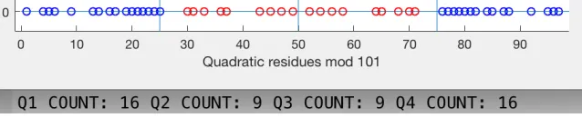
[image:31.612.147.466.556.621.2]Now we look at p = 17 = 4∗4 + 1, and create the same list. The QRs are 1,2,4,8,9,13,15,16. Sincen= 4, there are 3 QR’s in Quadrant I, 1 in Quadrant II, 1 in Quadrant 2, and 3 in Quadrant IV. Graphically, we can illustrate this forp= 101in Figure 3. The QR count is below the image.
Figure 3: A graph ofQR101.
Definition 14. Degree of Front-Loading modulop. The constant
ρ:= Number of QR’s in Quadrant II
Number of QR’s in Quadrant I (51)
is the Degree of Front-Loading modp. This tells us how biased the quadratic residues modpare.
For ease of discussion, also define the difference between the numbers of QR’s asξFormally,
Definition 15. Difference between QR counts.
The constant
ξ =Number of QR’s in Quadrant I−Number of QR’s in Quadrant II (52)
difference in QR’s from Quadrant I to that of Quadrant II.
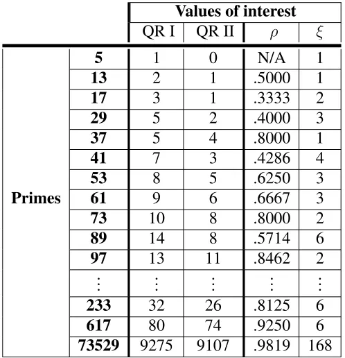
We directly computeρandξfor a few small primes in Figure 3 and carry it to primes less than 10,000 in Figures 4 and 5.
Values of interest
QR I QR II ρ ξ
Primes
5 1 0 N/A 1
13 2 1 .5000 1
17 3 1 .3333 2
29 5 2 .4000 3
37 5 4 .8000 1
41 7 3 .4286 4
53 8 5 .6250 3
61 9 6 .6667 3
73 10 8 .8000 2
89 14 8 .5714 6
97 13 11 .8462 2
..
. ... ... ... ...
233 32 26 .8125 6
617 80 74 .9250 6
[image:32.612.182.431.391.649.2]73529 9275 9107 .9819 168
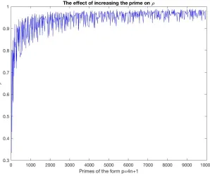
Figure 4: Howρis affected aspincreases
We see from Figure 4 that the values of ρ appear to be asymptotic toρ = 1,yet lim
p→∞ρ = 1
indicates that Front-Loading holds, however,ρis not monotonically increasing, despite being well aboveρ= 0.8for much of this figure. This means that the quadratic residues are relatively close in number for large primes. Ther However, this asymptotic nature seems to indicate that techniques
from analytic number theory may be helpful in proving this conjecture. Further, there does not
seem to be any sharpness in the graph, thus it is difficult to computeρalgebraically givenp. We also see from Figure 5 that less can be stated about the pure difference in QR’s other than
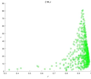
ξappears to be increasing in a general sense. Importantly to the case of Front-Loading,ξappears to be nonegative for all primes, supplemented by the general linear increase ofξ asp increases. However,ρandξappear to be uncorrelated, as shown in Figure 6. Do note again that most of the
ρcoordinates are larger than 0.8.
These constants further the argument that the quadratic residues are not uniformly distributed
7
An Algorithm to find the square root
We now will motivate and discuss the algorithm that we developed. The reader can find a working
MATLAB implementation in Appendix I of this thesis (Section 10). MATLAB has been used due
to its ease of use, portability, and easy to use tools to compute detailed runtime statistics to aid in
debugging/comparison. Letpbe prime, andC ∈ Z×
p. We want to determine whether or notC is
inQRp or inN Rp. If it is inQRp, we want to find the two square roots ofC. We will be heavily
using Theorem 3 and Corollary 4 from section 4.1 of this thesis.
Our algorithm is broken into two parts: Preprocessing and Perfect Square Multiplication. The
goal of preprocessing is to determine if a potential QR has an easy deterministic solution, or if it
is a NR. The remaining cases imply p = 8n + 1 and are difficult to assess. We will repeatedly multiply by carefully selected perfect integer squares to determine the square root of these cases.
The Front-Loading Conjecture, if it is true, will aid in selecting these integer squares quickly. See
Figure 7 for a visual representation of this.
Our algorithm beats brute force for large enough primes. We will be examining this in terms of
runtime and iteration count. Further, it is more transparent than the algorithms presented in Section
5, as it uses neither quadratic extensions nor the discrete log problem. These benefits allow our
algorithm to stand out and be useful in solving the square root problem, and we discuss potential
improvements to the algorithm’s design. We also discuss a replacement to the Preprocessing step
that allows the algorithm to avoid overflow inaccuracies. Importantly, implementing the algorithm
in a lower level language such as Python or C will improve the effectiveness of the algorithm by
getting around the dictionary and conversion ineffectiveness of MATLAB.
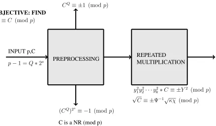
Now, we discuss the two major components of our algorithm in more detail, beginning with
CQ≡ ±1 (mod p)
C is a NR (mod p)
p−1 =Q∗2s
y2
1y22· · ·y2k∗C ≡ ±Y2 (mod p)
√
C ≡ ±Ψ−1√κχ (mod p) (CQ)2s
≡ −1 (mod p)
PREPROCESSING REPEATED
MULTIPLICATION
OBJECTIVE: FIND
x2 ≡C (mod p)
[image:36.612.95.534.73.330.2]INPUT p,C
Figure 7: The general flow of the algorithm
7.1
The Preprocessing steps
For preprocessing, we want to decide the quadratic character of potential quadratic residueC. As we will see in the remainder of Section 7, finding an efficient decidability condition in the repeated
multiplication step of the algorithm proves difficult, so this preprocessing proves important. We
could simply just use Euler’s Criterion, but to lower the strain on our machine we do this in stages.
We find
p−1 =Q∗2s, whereQis odd (53)
Qis easy to find as we are dividing by 2 as many times as possible. We then examineCQ. If this
is±1, we conclude that C is a quadratic residue. We can compute√Cas follows
CQ≡C∗CQ−1 ≡ ±1 (mod p) (54) √
CCQ−21 =± √
We note that this is a deterministic method to find the square root in these cases. We now prove
that this correct. We need to confirm that no NR will fall into this case.
Lemma 3. Quadratic character ofCifCQ≡ ±1 (mod p)
Letp= 4n+ 1 =Q∗2s+ 1. Then ifCQ ≡ ±1 (mod p), thenC ∈QR p
Proof. Letp= 4n+ 1 =Q∗2s+ 1, andC ∈N R
p. ThenQ= p2−s1. Sincep= 4n+ 1, s≥2.
Assume thatα=CQ ≡ ±1 (mod p). We can repeatedly squareα s−1times. so we have
α(2s−1) ≡(CQ)2s−1 ≡C(Q∗2s−1) ≡Cp−21 ≡1 (57)
And now we apply Euler’s Criterion (Theorem 4) to get the desired result.
Now, ifCQ ≡1 (mod p), thenC(CQ−1)≡1 (mod p), so√CCp−21 ≡ ±1 (mod p).
On an implementation note, in the case whereCQ ≡ −1, we use the method of Zagier [14] to
easily computep=a2+b2, and thus√−1via the extended Euclidean Algorithm [1].
IfCQ is not±1,then we will repeatedly square (mod p)this value, up tos−1times. If we
get1 at any point, says = k, then we know that C is a QR by the same logic as in the proof to Lemma 3. However,(CQ)2k
=C(CQ∗2k−1
). This exponent will be odd if2≤ k ≤ s−1, so we cannot perform the same trick we did above to easily find the modular square root. From this, we
can easily find√−1≡(CQ)2k−2
(mod p)as a direct consequence to Lemma 1
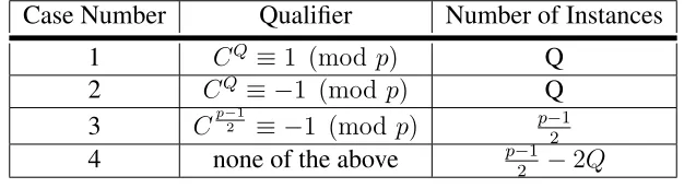
[image:37.612.149.462.531.617.2]This establishes four possible outcomes to this preprocessing. We state how this partitionsZ×p in Table 4
Case Number Qualifier Number of Instances
1 CQ≡1 (mod p) Q
2 CQ≡ −1 (mod p) Q
3 Cp−21 ≡ −1 (mod p) p−1
2
4 none of the above p−21 −2Q
Table 4: How the cases of preprocessing partitionZ×p
We now prove each of these instance numbers. Trivially, Case 3 follows Theorem 1. Cases 1
Theorem 14. 2Qmany instances ofCsatisfyCQ ≡ ±1 (mod p)
Letp= 4n+ 1 =Q∗2s+ 1, anda∈
Z×p. DefineAas follows:
A={C∈Z×p|CQ ≡1 (mod p)} (58)
Similarly, define
B={C ∈Z×p|CQ ≡ −1 (mod p)} (59)
Then|A| =|B| =Q
Proof. Letp= 4n+ 1andp−1 =Q∗2s. Thus,|
Z×p|=Q∗2sFurther, letgbe a primitive root
modp. Now leta=g2s. By Theorem 2,ord(a) = Q, and thus,|< a >|=Q.
Letγ ∈ A. Thus,γQ ≡1 (mod p). Thus,γ belongs to the unique cyclic subgroup of orderQin
cyclic groupZ×p. This unique subgroup of order Q is< a >. Further, considerar forr ≥1. Then consider
(ar)Q= (aQ)r= 1r = 1 (60)
due to Definition 5. Since the powers ofadefine< a >andar ∈ A, we can say that< a >=A,
and thus|A|=Q.
Now, similarly defineb =g2s−1. By Theorem 2,ord(b) = 2Q, and thus|< b >|= 2Q. Note that
sinceb2 ≡a (mod p),A={b2j|1≤j ≤Q}
((b2j−1)2)≡(a2j−1)Q (61)
We can thus see that every element that in < b > that is not in < a > is the square root of an element in< a >. But since this elementˆbis not inA, and thusˆbQ ≡√1, butˆbQ 6≡1or it would be in < a >. Now that the square root problem has exactly two solutions if a solution exists by Lemma 1, and(−1)2 = 1, soˆbQ ≡ −1and thusˆb∈ B.
In terms of set notation, we say thatB =< b >−A.
We further observe that since every other element of < b > goes to B andA, we see that A andB are disjoint, as expected by their definitions. Do note that this is an expansion to Turner’s
probabilistic proof for|A|=Q[16].
Thus we see that we can find a deterministic solution for 2Qof the quadratic residues modp. Thus there are p−21−2Qquadratic residues unaccounted for. We can deduce when2Qis maximal, among primes of the form4n+ 1.
Theorem 15. Size of2Qfor5 (mod 8)primes Letp= 8n+ 5 =Q∗2s+ 1. Then2Q= p−1
2
Proof. Letp= 8n+ 5 =Q∗2s+ 1. Via Algebra, we have,
p−1 = 22(2n+ 1) = 22(Q) (62)
and we are done
This means that all quadratic residues for p = 8n+ 5primes fall into these cases and have a deterministic solution to the square root problem. See [8] or Section 5 for Pocklington’s
determin-istic algorithm for these primes.
Applying this line of thinking to primes of the form4n+ 3produces a deterministic algorithm for finding the modular square root.
Corollary 5. Variation on the Cardinality of the sets of Reciprocity forp= 4n+ 3primes Letp= 4n+ 3 =Q∗2,+1, whereQ= p−21. Then only cases 1 and 2 in Table 4
Proof. Q= 2n+ 1 = p−21
Thus, we can incorporate deterministic results for all primes of the form 8n+ 1 This paints a more complete a more complete picture of prime modular behavior than Turner’s Result, as
turner ignores the case of CQ ≡ −1 (mod p). Thanks to Zagier-Shirali’s algorithm we have a
7.2
Crux of the Algorithm: The Repeated Multiplication
We now come up with a generic, yet easy to follow by hand algorithm to compute the square root
of a quadratic residue. We do not care whether or not the specific case would have been absorbed
in preprocessing. We do however, for this section, make the following two preconditions:
1. Primepis of the formp= 4n+ 1
2. Exclude case 3 in Table 4
Our goal is to repeatedly multiplyC by perfect integer squares until we arrive at a perfect integer square or its negative modulop. We provide pseudocode here. We use phrasing from the Front-Loading Conjecture (See Section 6.3)
1. INPUT:p= 4n+ 1, C ∈QRp
2. Initializeχ=C,Ψ = 1, κ= 1,
3. Whileχis not a perfect integer square and−χ (mod p)is not a perfect integer square: (a) ifχis not in Quadrant I or II updateχ≡ −χ (mod p), κ=−κ
(b) Select perfect integer squarey2
i such that±χyi2 (mod p)has yet to have been assigned
toχand updateχ≡χ∗y2i (mod p),Ψ≡Ψ∗yi (mod p)
4. if−χ (mod p)was the perfect integer square, updateχ≡ −χ (mod p), κ=−κ
5. Return
√
C ≡ ±Ψ−1√κχ (mod p) (63)
In full detail, we write the computation of√C as
(y21y22· · ·yk2−1y2k)C ≡√χ2 (mod p) (64)
(y1y2· · ·yk−1yk)
√
C ≡ ±√χ√±1 (mod p) (65) √
C ≡ ±(y1y2· · ·yk−1yk)−1
√
Theorem 16. Termination of repeated multiplication
Letp= 4n+ 1andC ∈QRp. Then there exist a finite sequence of integersyi such that
(y12y22· · ·y2k−1yk2)C≡√χ2 (mod p) (67)
We prove this in a few steps. We need a lemma first
Lemma 4. QR closure by integer squares.
Letp= 4n+ 1,C1, C2 ∈QRp. Then there exists an integeryisuch that
y2iC1 ≡C2 (mod p) (68)
Proof. From Theorem 3, we know thatQRpis closed. Thus there exists anxsuch that
xC1 ≡C2 (mod p), x, C1, C2 ∈QRp. (69)
Namely,x=C1−1C2. By Definition 4, sincex∈QRp, there exists aysuch thaty2 ≡x (mod p).
We substitute this into Equation 69 to get the desired result.
We now can prove that this overall process will terminate.
Proof. Letp= 4n+ 1andC ∈QRp. Note that1∈QRp. Via Lemma 4, one can pick any QR of
choice that has not been visited, and find a perfect integer square to visit that QR. Due to Theorems
1 and 3 (namely the fact that|QRp|is finite), one must visitχ= 1at some point and the algorithm
will terminate.
Due to the fact that the algorithm only modular multiplication, this algorithm avoids all of the
advanced calculations and much of the trial and error that is present in Tonelli-Shanks, Cipolla,
and Pocklington’s algorithms [8, 15]. Further, the algorithm can be sped up since we are always
looking at the value ofχor it’s negative as allowed to us by Corollary 4. However, this is dependent on the strategy that one uses to picky2
i. The strategy that we have implemented is predicated on
the fact that Quadrant I contains more perfect integer squares and the Front-Loading Conjecture.
Conjecture 2. Optimal selection ofy2 i
Select the least integerksuch that
y2i = "s
kp χ
#2
, k ∈N (70)
corresponds to a χy2
i (mod p) has yet to be visited in the proceedings of the algorithm and this
χy2
i is in Quadrants I or IV, where[x]in this case roundsxto the nearest integer.
It is important to note that thisχy2
i has yet to be visited. If this was not the case, the algorithm
would infinitely loop. To avoid this, k can increase as needed, creating a “moving goalposts” approach to finding a perfect integer square that will work. Takep = 17, C = 8for example. The integer square that would be found is y1 = 1, which would obviously cause a loop as χ would
never leave 8. Other examples could create a loop that does not includeC itself. Illustrating this is a case wheny2
my2m+1· · ·yn2 ≡1 (mod p)There are other strategies, but we will discuss them in
Section 7.4.
We want to maintain that we can picky2
i quickly. This is the place of Front-Loading. Because
there are more Quadratic residues in the ’RICH’ half ofZ×p, if we pick ay2
i randomly, we are more
likely to land in Quadrants I and IV. Further, this likelihood increases asξ, ρincrease. Further, This choice ofy2
i will help terminate the algorithm quickly, as this will put the corresponding±χyi2 (mod p)as close to0 (mod p)as possible. As the perfect integer squares are concentrated about
0 (mod p), this choice ofy2
i will help facilitate that .
Lastly, we would like to address this constant shifting to quadrants I and II.The largerχis, the closer kpχ is tok ∀k. This will decrease the speed in which we can selecty2
i, as candidate values
ofkwill need to be larger than that of the samek, but with a smallerχ. This shifting is once again allowed to us by Corollary 4 However, on the note of Quadrant II, by how we are choosing y2
i,
once we leave Quadrant II, we will never return. This implies that if we ever use Quadrants II or
III, thenC is in one of these quadrants.
We noted that since the number of QR’s are finite, however this will form the basis of the
7.3
Comparing our algorithm to Brute Force
In this section, we discuss the overall effectiveness of our approach and compare it to brute force.
We will do this in two ways. In terms of sheer runtime, we will be using MATLAB’s profiling
tool, as using the tic/toc and cputime functions can be buggy or misleading in our experience. We
avoid measuring our algorithm in terms of Big-Oh notation, deferring to practical observables from
implemented computation. This is the major portion of the algorithm, as the Square and Multiply
algorithm and the Extended Euclidean Algorithm are sublinear in this respect. What you will see
in this analysis is a function that we have written called TestSuitev2. This function takes in a prime,
a number of random elements inZ×p to test against brute force, and a trigger quantifying if we only want to test QRs (1), NRs(0), or a random mixture of the two (-1), in this order. We present sample
[image:43.612.220.394.325.479.2]output in Figure 8.
Figure 8: Running 10,000 random trials forp= 73529to see runtime
Due to the segmented nature of preprocessing, we break this into primes of the formp= 8n+1
and everything else. We now present p−21 mixed trials in Tables 5 and 6
This shows that it appears that our algorithm does not run well for small primes, but does well
for large primes. In the first case, it appears that our algorithm does better for primes larger than
approximately3500, and approximately1000for the second case. If a more concrete number could be found, we would be happy. We then have the following statement
Conjecture 3. Beating brute force with our algorithm.
p AlgoRuntime Brute-force Runtime
17 .010s .001s
97 .016s .002s
617 .047s .018s
977 .081s .043s
1361 .115s .080s
2377 .260s .246s
3041 .378s .414s
3313 .484s .482s
[image:44.612.194.421.71.224.2]4721 .594s 1.023s
Table 5: Comparing runtimes for1 (mod 8)primes
p AlgoRuntime Brute-force Runtime
13 .009 .001s
101 .013s .002s
283 .017s .006s
503 .026s .013s
1061 .054s .050s
1999 .090s .175s
2029 .096s .184s
6053 .333s 1.646s
Table 6: Comparing runtimes of other primes
Thus, the sheer number of possibilities appear to hamper brute force compared to the algorithm
and this selection ofy2
i. This shows that the algorithm is not perfect for every4n + 1prime, but
does indeed beat brute force ifpis large enough.
We believe that there are two major things that slow the algorithm down. These are the square
and multiply algorithm and dictionary use in MATLAB. Recall that the Square and Multiply
algo-rithm should be running sublinearly. If we return to examining Figure 8, let us look at the most
time consuming steps of the algorithm in Figure 9 (this was forp = 73529 ≡ 1 (mod 8)). Note that we call our dictionary of previously visited values “prev”.
[image:44.612.194.420.259.398.2]Figure 9: The most time consuming steps of the algorithm
Conjecture 4. Lower level language implementation.
Implementing our algorithm in a lower level language will reduce the value ofwin Conjecture 3 When it comes to the Square and Multiply algorithm, most of the runtime is spent converting a
number into binary. This is done via thestr2doublecommand (we have implemented str2doubleq to make things a little better [4])
Supplementing this argument is an argument on the average number of iterations. This is a
rather nebulous term to define. We do this for brute force and our algorithm below. In general,
we are incrementing this iteration counter whenever a for/while loop, well, loops. We ignore
preprocessing for our algorithm because, again, it should run sublinearly due to the square and
Multiply Algorithm and repeated squaring. Recall thatC is our candidate Quadratic residue. For this discussion, we assume thatCis indeed a quadratic residue.
Definition 16. Iteration for brute force
We define one iteration for brute force as every integer that we square and compare toC.
Definition 17. Iteration for our algorithm
We define one iteration for our algorithm as every instance we compute an invalidy2i, and every time we update our bookkeeping forΨ.
the argument in the grand scheme of things. We are using our own built function to compute
this. We also have built our own function that performs just the repeated multiplication step of the
algorithm. As before, we show one sample output in Figure 10,
Figure 10: Running 10,000 random trials forp= 73529to see iteration count
before extrapolating this and showing results for various primes in Table 7. We do not care of
the form of the prime other than it must be of the form4n+ 1.
p Total Algo iters Average Algo iters Total Brute-force iters Total Brute-force iters
13 6 1 8 1.3333
17 6 0.75 35 4.375
97 184 3.8333 1200 25
101 275 5.5 1067 21.34
617 2581 8.3799 48927 158.8539
977 6240 12.7869 116519 238.7684
1999 44716 44.7608 505815 506.3213
1361 8061 11.8544 232521 341.9426
2377 38752 32.6195 693200 583.5017
3041 36637 24.1033 1168862 768.9882
4721 65538 27.7703 2784188 1179.7407
[image:46.612.76.541.291.491.2]6053 128021 42.307 4691574 1550.421
Table 7: Comparing iterations for various4n+ 1primes
This shows a few things. Most importantly, the total number of iterations seems to be far less
than that of brute force. This forms our heuristic argument that if implemented in a lower level
language, our algorithm should be able to beat brute force for smaller primes, as well as larger
ones. We graph these average iteration count for brute force and repeated multiplication in Figure
11 to strengthen this. Notice how small the average number of iterations grows incredibly slowly
for repeated multiplication.
Figure 11: Average number of iterations for brute force vs. repeated multiplication
number of updates toΨ. This was based on the number of non perfect integer square quadratic residues, with the front loading conjecture allowing us to selecty2
i without much issue. However,
especially for large primes, our algorithm seems to perform much better than this.
Taking these two measurement methods into account, measuring by runtime shows that our
algorithm beats brute force in terms of runtime for large primes. Conjecture 4 will seem to be our
out to make our algorithm beat brute force in all cases. Measuring in terms of iterations seems
much more promising to showing that our algorithm is better than brute force.
The question now becomes if there are ways to improve the design itself of the algorithm. We will
see that we do not believe that there is a trivial way to do so, so our algorithm is ideal to find the
modular square root when it exists, and to decide upon the quadratic character of a number quickly
7.4
Improving the Design of the Algorithm
Further, there are two ways to try improve the algorithm that we see from a design perspective.
The first way to improve the algorithm’s design is to attempt to better incorporate the preprocessing
steps into the design of the algorithm. Let us first try to fix preprocessing before trying to replace it.
As the iteration comparisons are related to repeated multiplication exclusively, we will use runtime
to make the assertions we will for this improvement.
Perhaps, it would be faster to just compute Euler’s Criterion and run repeated multiplication on the
QR’s. This however, is not shown by the empirical data. We show this in Table 8, which takes both
decidability and removing these easy cases by using a mixture of QR’s and NR’s.
p Algo Runtime Euler’s Criterion Runtime
17 .008 .009
97 .017 .014
101 .013 .014
617 .049 .059
977 .090 .104
1361 .119 .141
[image:48.612.179.436.280.406.2]6053 .338 1.153
Table 8: The runtime effects of just using Euler’s Criterion
This gap seems small for small primes, but grows as p increases. We believe that ruling out the easy cases of QR’s rather than making the effort of engaging repeated multiplication gives our
preprocessing the edge here.
A less trivial attempt that we have made is an approach inspired by the Collatz Conjecture. One
can find its implementation in Section 10 for those looking for details on how it works. Basically,
it is built on many subcases and driving C down to a perfect integer square. However, empirical data is not on its side either. See Table 9.
For smaller primes, this approach seems close to/sometimes beating brute force. However, as
p increases, the regular version of preprocessing takes the lead. However, all is not lost for this Collatz Preprocessing. One major advantage that it has to our preprocessing is that overflow is
p Algo Runtime Collatz Version Runtime
17 .012 .009
97 .017 .012
101 .012 .014
617 .050 .042
977 .092 .087
1361 .116 .120
[image:49.612.180.429.71.197.2]6053 .343 .949
Table 9: The runtime effects of just using a Collatz approach to preprocessing
We also came up with a method that performs a depth first search between integers that have
the quadratic character, however, this renders the transparency argument moot, the runtime won’t
probably be improved much due to having to generate the graph and then perform depth first search
and we found it difficult to implement efficiently.
The reader may have noticed that the preprocessing appears to be independent of the repeated
multiplication.This is due to the fact that none of the decidability conditions we discovered for the
repeated multiplication itself are feasible at a fast runtime or number of iterations. The first of
these attempts is to find an upper bound fory2i. We note that
Theorem 17. Consecutive set ofQRp
Letp= 4n+ 1be prime. ThenQRp ={12,22,32· · ·(2n−1)2,(2n)2}
Proof. Letp= 4n+ 1and1≤α, β ≤2n. Further, assumeα2 ≡β2 (mod p). Then
α2−β2 =kp, k∈Z (71)
Thus,
p|(α−β)(α+β) (72)
By the prime propertyp|(α−β)orp|(α+β).
Assumep|(α+β). Due to the fact thatα, β ≤2nmeans that this can be at mostp−1. By this and the lower bounds ofα, β, we can say that
And note that no multiple ofplies in this interval. This contradicts the fact thatp|(α+β). Let us now consider the other possibility. By the same logic, we can say
0≤ |α−β|< p (74)
Thus, the only way forpto divide|α−β|if if
|α−β|= 0, → α=β (75)
this means that for all QR’s generated byα2 are uniquely defined for1 ≤ α ≤2n. This provides
2n total QR’s in this interval. Theorem 1, also gives that there are 2n QR’s total. Thus, by the pigeonhole principle, we have the expected result.
This m