Influence of physical road characteristics on road crashes

(1)

INFLUENCE OF PHYSICAL ROAD

CHARACTERISTICS ON ROAD

CRASHES

JASON JENSEN

BENG

(2)

(3)

University of Southern Queensland

Faculty of Engineering and Surveying

Influence of Physical Road Characteristics

on Road Crashes

A dissertation submitted by

Jason W. Jensen

in fulfilment of the requirements of

Courses ENG4111 and 4112 Research Project

towards the degree of

Bachelor of Engineering (Civil)

(4)

Abstract

The objectives of this project were to find correlations between the ‘tidal flow’ of traffic

and the frequency of road crashes, as well as between various broad scale road

environment factors and the frequency of road crashes. This was achieved through an in

depth examination of crash data for the Southern District, as well as the combined data

of the areas covered by the Toowoomba City Council and the Gatton Shire Council.

When examining the data for correlations, the traffic flow and crash rate along with

various road environment characteristics were considered.

It was found that a greater traffic flow did not mean a greater crash rate would result

with the time periods with lower traffic flow having higher crash rates. However,

correlations were established between various road environment factors and the

frequency of road crashes. Road environment characteristics that were found to

influence the amount of road crashes included the seal width, pavement width,

formation width, the speed limit zones and the AADT of the road. These correlations

(5)

University of Southern Queensland

Faculty of Engineering and Surveying

………….ENG4111 & ENG4112

Research Project

……….

.

Limitations of Use

The Council of the University of Southern Queensland, its Faculty of Engineering and Surveying, and the staff of the University of Southern Queensland, do not accept any responsibility for the truth, accuracy or completeness of material contained within or associated with this dissertation.

Persons using all or any part of this material do so at their own risk, and not at the risk of the Council of the University of Southern Queensland, its Faculty of Engineering and Surveying or the staff of the University of Southern Queensland.

This dissertation reports an educational exercise and has no purpose or validity beyond this exercise. The sole purpose of the course pair entitled "Research Project" is to contribute to the overall education within the student’s chosen degree programme. This document, the associated hardware, software, drawings, and other material set out in the associated appendices should not be used for any other purpose: if they are used, it is entirely at the risk of the user.

Prof G Baker Dean

(6)

Certification

I certify that the ideas, designs and experimental work, results, analyses and conclusions

set out in this dissertation are entirely my own effort, except where otherwise indicated

and acknowledged.

I further certify that the work is original and has not been previously submitted for

assessment in any other course or institution, except where specifically stated.

Jason Jensen

Student Number: Q11224289

Signature

(7)

Acknowledgements

For their technical support I would like to thank Mr Mal McIlwaith from Queensland

Transport for sourcing and supplying me with the crash data and sharing with me his

ideas on the topic and Associate Professor Ron Ayers for his guidance and advice when

I first started the undertaking of this project. Finally I would like to thank my family

and beautiful girlfriend for their support, encouragement and belief because without

them I would never have made it this far.

J. Jensen

University of Southern Queensland

(8)

List of Figures

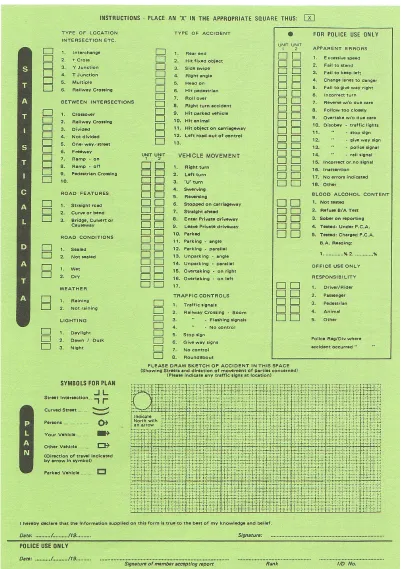
Figure 2.1: Appropriate Road Crash Report Form ... 7

Figure 2.2: Involvement of Factors in Accidents ... 12

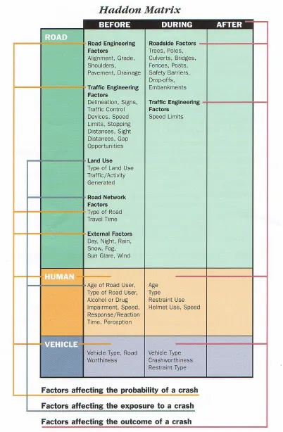
Figure 2.3: The Adapted Haddon Matrix for Road Crashes... 14

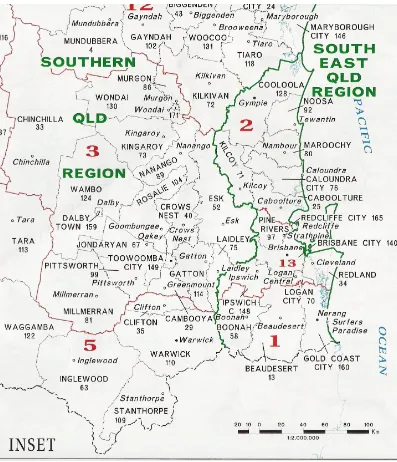
Figure 3.1: Location of Southern District in Queensland... 17

Figure 3.2: Detailed View of the Southern District ... 18

Figure 4.1: Initial Crash Data file containing Four Districts... 30

Figure 4.2: ‘Local Government Authority’ Identification... 31

Figure 4.3: Identifying Crash Road ‘RsectID’... 32

Figure 4.4: Chainage Distance, ‘TDIST’, of the Road ... 32

Figure 4.5: Road Data Matching Crash Data Above ... 33

Figure 4.6: Direction of Travel factor used to determine Carriageway ... 34

Figure 6.1: Double Lane Sealed Shoulders – Toowoomba and Gatton... 48

Figure 6.2: Four Lane Sealed Shoulders – Toowoomba and Gatton... 48

Figure 6.3: Double Lane Sealed Shoulders – Southern District ... 49

Figure 6.4: Four Lane Sealed Shoulders – Southern District... 51

Figure 6.5: Single Lane Pavement Width – Toowoomba and Gatton... 53

Figure 6.6: Double Lane Pavement Width – Toowoomba and Gatton ... 53

Figure 6.7: Single Lane Pavement Width – Southern District ... 54

Figure 6.8: Double Lane Pavement Width – Southern District ... 56

Figure 6.9: Single Lane Formation Width – Toowoomba and Gatton... 58

Figure 6.10: Single Lane Formation Width – Southern District... 60

Figure 6.11: Double Lane Formation Width – Southern District ... 60

Figure 6.12: Speed Limit Zone Crashes – Toowoomba and Gatton ... 62

(12)

List of Tables

Table 5.1: Tidal Flow – Toowoomba and Gatton ... 39

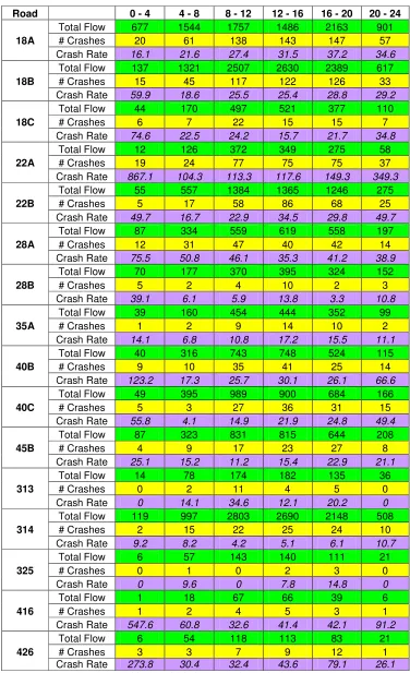
Table 5.2: Tidal Flow – Southern District ... 42

Table 6.1: Seal Width Crashes/Km – Toowoomba and Gatton... 47

Table 6.2: Seal Width Crashes/Km – Southern District... 50

Table 6.3: Pavement Width Crashes/Km – Toowoomba and Gatton... 52

Table 6.4: Pavement Width Crashes/Km – Southern District ... 55

Table 6.5: Formation Width Crashes/Km – Toowoomba and Gatton... 57

Table 6.6: Formation Width Crashes/Km – Southern District... 59

Table 6.7: Speed Limit Zone Crashes/Km – Toowoomba and Gatton ... 61

Table 6.8: Speed Limit Zone Crashes – Southern District ... 62

Table 6.9: AADT vs. Width - Double Lane Sealed Shoulders Southern District... 65

Table 6.10: AADT vs. Width - Single Lane Pavement Toowoomba and Gatton ... 66

Table 6.11: AADT vs. Width - Single Lane Pavement Southern District ... 67

Table 6.12: AADT vs. Width – Double Lane Pavement Southern District... 68

Table 6.13: AADT vs. Width - Single Lane Formation Toowoomba and Gatton... 69

Table 6.14: AADT vs. Width - Single Lane Formation Southern District ... 71

(13)

Chapter 1

Introduction

1.1 Aims of Project

This project is a result of Mal McIlwaith from Queensland Transport and his interest in

the road environment and its involvement of road crashes. He is also interested in

whether or not it plays a larger role than is currently thought in crashes. This project has

then, in turn, evolved from this query.

The usual approach to investigating road crashes is to report on the characteristics that

are specifically related to the drivers of the vehicles involved in the accident. This

project investigates if certain road environments play a larger role in accidents than is

(14)

The initial aim of this project was to find a correlation between the ‘tidal flow’ of traffic

and the frequency of road crashes. The percentage of heavy vehicles in this ‘tidal flow’

also had to be considered.

The major aim was to find correlations between various broad scale road environment

factors and the frequency of road crashes. These correlations were then used to predict

the likely crash zones of roads.

1.2 Dissertation Overview

The second chapter of this dissertation gives a background on the project undertaken

and also uses a literature review. This review reveals information gained in previous

studies relating to the issues of crash data analyses and the correlation of crash rates

with influencing parameters.

The third chapter gives an explanation of Southern District and the features of the

district such as the size, towns and local government areas included within the

boundaries. It also incorporates the road types that are examined with specific examples

of these roads.

The fourth chapter describes the three types of data that were required to be analysed in

this project. These three data sets were the crash data, road data and the Southern

District traffic census. The methodology used to complete the project is also outlined,

(15)

The fifth chapter reports on the analysis of the factors relating to the ‘tidal flow’ of

traffic and the crash rate. The crash rate, crashes per one million vehicles, for time

periods of four hours on certain roads in each area was found. Then it was compared to

the other roads and the tidal flow of traffic during these periods

The sixth chapter reports on the analysis of the factors relating to the road environment

and the frequency of road crashes. The factors that were analysed as part of the road

environment included the seal width, pavement width, formation width, speed limit

zones and the AADT vs. Width.

Chapter seven discusses the results gained from the previous two chapters. Each section

compares the results of the analyses for each study area. They then go on to report on

any correlations that were found concerning the factor that is discussed in each section.

Chapter eight includes conclusions and recommendations from the analysis of the data

as well as any further work that could be continued on with as a continuation of this

(16)

Chapter 2

Background Studies

2.1 Introduction

This chapter gives a background on the project undertaken and how it started. It then

goes on to a use a literature review. This review reveals information gained in previous

studies relating to the issues of crash data analyses and the correlation of crash rates

with influencing parameters. It also looks at the similarities and differences between

(17)

2.2 Background

The usual approach to investigating road crashes is to report on the characteristics that

are specifically related to the drivers of the vehicles involved in the accident. This

project investigates if certain road environments play a larger role in accidents than is

currently understood.

This project is a result of Mal McIlwaith from Queensland Transport and his interest in

the road environment and its involvement of road crashes. He is also interested in

whether or not it plays a larger role than is currently thought in crashes. This project has

then, in turn, evolved from this query.

2.3 Literature

Before any work could commence on this project, there was a need for a review of

literature. This literature is in two specific areas: the analysis of crash data and the

correlation of crash rates with influencing parameters. These two issues are

comprehensively examined below through the use of a literature review.

2.3.1 Crash Data

Crash data describing accidents occurring on Australian roads, has been collected since

(18)

data until early 1989 when this responsibility was transferred to the Statistics

department of Queensland Transport.

In Austroads (2004) it is noted that if the data recorded is to be considered good, and

therefore useful to users of this data, it must be able to achieve various factors. These

factors are as follows:

• crash sites can be located accurately,

• the succession of events occurring throughout the accident sequence are able to

be determined,

• contributing factors to the crash can be established; and

• common factors relating a number of crashes can be ascertained.

These are considered important so that when the data is analysed for various reasons, it

is as complete as possible to be able to determine, for example, if a certain section of

road is a problem area or “a black spot”. NAASRA (1988) has a recommended road

(19)

[image:19.612.132.533.49.618.2]

Figure 2.1: Appropriate Road Crash Report Form

(20)

In NAASRA (1988) there are several suggested potential sources that crash data can be

obtained from. However, the most commonly accepted and used source from the given

range of choices are the Police Road Crash Reports. It is important to understand that

not all crashes are reported and there are specific requirements for reporting accidents.

NAASRA (1988, p.13) explain that these guidelines in Queensland are,

“all casualty crashes, and property damage crashes where the estimated cost

of damage exceeds $1000.”

The minimum figure stated above (damage exceeding $1000) for reporting an accident

was raised in December 1991 to an amount of $2500 (Bureau of Transport and

Communications Economics, 1995). The crash data is recorded from reported accidents

that meet the criteria established above.

Austroads (2004) have stated that a road crash is made up of three components that

interact. These components are listed as the human factor, the vehicle factor and the

road factor. Austroads have defined that

“a crash or accident may be considered as a ‘failure’ in the system”

(Austroads, 2004, p.10).

In general, road crash data is analysed using factors that influence the accident, which

are then recorded. According to Queensland Transport (2002) and the Victorian

Transport Accident Commission (2004), the common factors that are used by these two

organizations are the age and gender of involved parties, the type of transport in the

(21)

factors contributing to the crash. Characteristics of crashes concern information

regarding the number of vehicles involved in the accident, the time of day and week

when the accident happened and if the accident occurred in a metropolitan or rural area.

According to Queensland Transport (2002), the major factors contributing to crashes are

alcohol involvement, speed, fatigue and seat belt usage.

Symmons, Haworth and Johnston (2004), also used the above statistics when analysing

road crashes but also extended these factors to include a limited investigation of the

road characteristics of the accident site. These extended factors include if the location

was an intersection or not, the road alignment (i.e. if the road was a straight or part of a

curve etc.) and if it was a divided or undivided carriageway. The factors included by

Symmons, et al. involving the road characteristics will be analysed when the Southern

District data is analysed. However these factors will be increased to include more

information about the road environment. These increased factors will include such

information as road width, seal type etc. as recommended by NAASRA (1988).

Although NAASRA (1988) also suggests that when investigating accidents, the above

human or driver influencing factors be used, they also recommend that the investigation

be taken further by using relevant site conditions including those described in the

previous paragraph. In particular, the most important of these conditions are road,

lighting, road surface and visibility. The road factor is the most detailed including

features such as width, number of lanes, markings, camber and gradient. Lighting and

visibility are as they imply, with lighting describing the illumination of a section of

pavement at nighttime and visibility referring to the distance and quality of a drivers

view. Finally the road surface factor concerns the type of surface, condition of the

(22)

characteristics in their analysis and NAASRA (1988) recommended that a number of

road environment details that can and will be analysed in more depth. These factors

relating to the road environment will be included in the investigation of the influence of

the physical road characteristics on road crashes.

Hutchinson (1987) suggests that Great Britain, South Australia, Western Australia and

most states of U.S.A also only collect the information that both Queensland and

Victorian departments use to analyse crash data. Although the information from

Hutchinson appears to be outdated, it can be seen through recent literature from

Queensland and Victoria transport departments, that government departments do not use

any data concerning the road environment when analysing road crashes. This project,

will therefore attempt to develop a correlation between road environments, many factors

of which are rarely considered by government departments, and road crashes.

2.3.2 Correlation of Influencing Parameters

The first and often the most examined characteristics are the age and gender

characteristics of drivers. According to Queensland Transport (2002) the age category,

of three year intervals, that is involved in the most amounts of road crashes is the 17 to

20 year old bracket. Expanding to this category it can also be seen that the group of 17

to 24 year olds, males make up about 85% of the total. Symmons et al. (2004) found

that those under the age of 25 years old were the largest group involved in accidents but

were mostly passengers. However the drivers that were most involved were in the 25 to

39 year old category. It was agreed that males made up the greatest amount of road

(23)

Contrary to the results above was the amount of higher age (above 35) drivers involved

in accidents in rural Victoria. Symmons et al. (2004) discovered that in rural Victoria

accidents at intersections accounted for 37% of crashes. It was also found that only

21% of crashes occurred on curves. The accidents at intersections were the least severe

and accidents on curves were the most severe. However, there were a low percentage of

accidents taking place on curves.

Of the factors contributing to crashes alcohol was the most common factor according to

Queensland Transport (2002), with disobeying traffic following narrowly behind.

Trailing these were inexperience, speed and then a lack of concentration.

The correlations discussed above are mostly about accidents where the human factors

causing accidents are analysed. The remainder of this section details studies that

investigated the impact of the road environment on accidents. The Bureau of Transport

and Communications Economics (1995) stated that the demands that the road

environment places on a driver are dependent on the flow of traffic, geometric design

features of the road and also the type of road being used. The Bureau of Transport and

Communications Economics Bureau (1995) also believes that the performance of the

driver needs to increase as the demands of the road environment, which is put on the

driver, also increases. Hence, it is when the performance off the driver does not meet

the demand of the road environment that road crashes occur.

The Road and Traffic Authority (1996) illustrate how each of the three components of

the transport system contributes to road crashes. The Human Factors causing a crash is

95%, the Road Environment contributing 28% of the time and various Vehicle factors

(24)

is the sole cause in 4% of accidents and is a contributing factor when combined with

[image:24.612.166.496.126.346.2]

Human factors 24% of the time.

Figure 2.2: Involvement of Factors in Accidents

(Source: Road and Traffic Authority (1996))

The road environment features above were found to be influenced by:

• Road and road side engineering,

• Traffic management; and

• Transport and land use.

Of these factors it can be seen from the Haddon Matrix, Figure 2.3 that before an

accident occurs the factors affecting the probability of a crash are:

• Road Engineering factors,

• Traffic Engineering factors,

(25)

• Road Network Features; and

• External factors.

Of these factors, roadside factors and traffic engineering are still factors at work when

an accident is occurring.

As mentioned earlier, road side engineering is a consideration included in the road

environment. A report by Kloeden, McLean, Baldock and Cockington(1999), on road

side hazards, concluded that in 39% of accidents between 1985 and 1996, a road side

hazard played a part in fatal accidents. It was also concluded that 38% of

hospitalizations between 1994 and 1996 involved an accident involving a road side

hazard.

From these conclusions it was recommended by Kloeden et al. (1999) that as the road

environment plays a large role in keeping motorists from running off the road, a number

of improvements should undertaken with respect to the road environment to assist in

this. The aspects of the road environment that were recommended to be improved were

the horizontal alignment of the road, an upgrade of the road surface condition and

(26)

[image:26.612.132.534.51.665.2]

Figure 2.3: The Adapted Haddon Matrix for Road Crashes

(27)

2.4 Chapter Summary

This chapter has given a background on this project and how it began. After the

background had been established the literature review revealed information gained from

past studies on the issues of the analysis of crash data and the correlation of crash rates

with influencing parameters.

From the literature review, it was seen previous studies have been undertaken showing

that various road environments can be contributing factors to a crash. In spite of these

findings very few, if not any, state or federal authorities examine any road data relating

(28)

Chapter 3

Southern District

3.1 Introduction

As the area of investigation for this project is the Southern District of Main Roads, an

explanation of this area is necessary to fully understand the results found. This chapter

includes the features of the district such as the size, towns and local government areas

included within the boundaries. It also incorporates the road types that are examined

(29)

3.2 Size

The area that is classified as the Southern District by Main Roads is a parcel of land

that is located on the western edge of South East Queensland, district number three in

Figure 3.1. The most western point of the Western boundary is positioned

approximately twenty-five kilometres to the west of Chinchilla and the corresponding

point to the East is situated approximately twenty kilometres North of Ipswich. The

[image:29.612.205.466.316.621.2]

distance that spans between these points is roughly 250 kilometres.

Figure 3.1: Location of Southern District in Queensland

(30)

In the North-South direction, the span is almost 300 kilometres with the most Southerly

part of the boundary being thirty-five kilometres South of Millmerran and to the North

[image:30.612.134.531.153.615.2]

this point is about 125 kilometres North of Chinchilla (Figure 3.2).

Figure 3.2: Detailed View of the Southern District

(31)

3.3 Towns and Local Government Areas

3.3.1 Towns

With the Southern District being as large as it is, it is obvious that there are numerous

towns in this area. Most towns are only small rural centres but there are a few larger

towns of note. These are Murgon, Kingaroy and Nanango to the North, Chinchilla and

Dalby to the West, Gatton, Laidley and Esk to the East and Millmerran and Pittsworth.

The largest and perhaps most important town in the District, which can be classed as a

city, is found centrally in the investigated area. This city is Toowoomba and it is also

found along with the one other centrally located town of Crows Nest.

These towns discussed above are considered small rural towns when compared to

centres such as Brisbane. The only exception in the entire district is Toowoomba,

being much larger than the other towns. Most of the towns above are the principal

towns of the shires listed below.

3.3.2 Local Government Areas

Within the southern District there are seventeen different Local Government Areas, as

seen in Figure 3.2. Working from North to South they are:

• Chinchilla,

• Wondai,

• Murgon,

(32)

• Nanango,

• Wambo,

• Rosalie,

• Dalby Town,

• Crows Nest,

• Esk,

• Gatton,

• Laidley,

• Toowoomba City,

• Cambooya,

• Jondaryn,

• Pittsworth; and

• Millmerran

Most of these shires are rural shires that have to service large areas which contain

substantial amounts of roads. More often than not, these shires have restricted budgets

that need to be used with careful consideration. However, roads are not the only

consideration that these councils need to acknowledge when determining where the

funds from their respective budgets are to be spent. As a result, roads can often fall into

a below satisfactory condition. The only local authority, from the list above, that has a

large budget is the Toowoomba City Council. However, the Toowoomba City Council

has a minimal amount of roads that are considered throughout this study, and as a

result, minimal maintenance is required.

As a comparison of budgets that councils have available to spend on roads the

(33)

compared. In the Financial year of 2002/2003 Kingaroy Shire Council had an

expenditure of approximately $2.272 Million on maintenance and construction

(http://kingaroy.qld.gov.au, 2004) and the Toowoomba City Council, in the same

financial year, spent $11.04 Million (http://www.toowoomba.qld.gov.au, 2004). This

demonstrates the different levels of funds available for expenditure on roads that exists

between the rural shires and city councils.

3.4 Road Types

There are three different types of roads that are examined in the Southern District of

Main Roads for the purposes of this project. These are state highways, main roads and

secondary roads, all of which are described in more detail below.

3.4.1 State Highways

State highways according to the NAASRA Road Classification System (refer to

Appendix C1) is a Class 1 road which is described as:

“those roads which form the principal avenue for communications between

major regions of Australia, including direct connections between capital

cities.” (Bureau of Transport and Regional Economics, 2003)

in the road data, these road classifications range from national highways to state

(34)

B, classifies roads as state highways with numbers 10 – 49. These numbers are usually

followed by a letter ‘A’, then successively progressing through the alphabet. These

letters represent a particular section of the road as the highways pass through many

towns. In the case of 18A, the Warrego Highway, the ‘A’ represents the section of

highway between Ipswich and Toowoomba then 18B is the section from Toowoomba

to Dalby.

Examples of these roads are, as mentioned above, the Warrego Highway, which travels

between Brisbane and Miles. Another example is the New England Highway which

starts in Yarraman and travels to Warwick and a final example is the Gore Highway,

running from Toowoomba to Goondiwindi. A full list of these roads and the

corresponding section is included in Appendix B1.

3.4.2 Main Roads

Main roads are defined as Class 2 in the NAASRA classification system (Appendix C1)

which explicitly defines these roads as:

“those roads, not being Class 1, whose main function is to form the principal

avenue of communication for movements:

•Between capital city and adjoining states and their capital

cities; or

•Between a capital city and key towns; or

•Between key towns.” (Bureau of Transport and Regional

(35)

the classification received by these roads in the road data is either regional roads or

district roads. In terms of Main Roads categorisation, main roads are classified using

numbers 100 – 999. Unlike state highways these roads are not followed by any

lettering system. This is because these roads consist of only one section.

Main roads generally are roads that connect two towns and thus, take their name from

the towns that the road connects. This is by far, the most common road type in the

Southern District. Examples of this type of roads are the Oakey – Cooyar Road, Esk –

Kilcoy Road, Gatton – Helidon Road and Chinchilla – Tara Road. A complete list

containing all of the Main Roads and classifications can be found in Appendix B2.

3.4.3 Secondary Roads

Asecondary road according to NAASRA is:

“those roads, not being Class 1 or 2, whose main function is to form an

avenue of communication for movements:

•Between important centres and the Class 1 and Class 2 roads

and/or key towns; or

•Between important centres; or

•Of an arterial nature within a town in a rural area”

(Bureau of Transport and Regional Economics, 2003)

the road data also refer to these roads as either regional roads but most often are

(36)

is a number between 1000 – 9999. These roads are much like main roads in the respect

that they are also roads that join neighbouring towns. However, the towns they join are

not as significant. The major difference between main roads and secondary roads, is

that secondary roads carry less traffic and therefore are not as frequently used.

Examples of these roads include the Millmerran – Cecil Plains Road, Murphy’s Creek

Road and Bunya Mountains Road.

3.5 Chapter Summary

This chapter has described the area analysed in this project, the Southern District. The

first factor relating to the Southern District that was analysed was the size of the district.

This revealed the district to be approximately 250 kilometres by 300 kilometres (at

maximum distances) in area. Next, the towns and local government areas were reported

on, from this it was found that there were seventeen different local government areas in

the district. The major towns in the district were also found to be the principal towns of

these areas.

Finally, the different types of roads in the district that were of significance were

described. There are three different classes of roads contained in the Southern District

that were to be considered in the analysis. They were state highways, main roads and

secondary roads. In the descriptions of these three road classifications, a description

from NAASRA was specified for each, the classification method as used by Main

(37)

Chapter 4

Data and Methodology

4.1 Introduction

This chapter describes the three types of data that were required to be analysed in this

project. These data sets were the crash data, road data and traffic census data. After the

types of data are described, the methodology used to complete the project was outlined,

explaining how each stage was completed. The steps that were undertaken throughout

the work carried out in this project included how the data was obtained, the initial work

undertaken on crash data, the correlation of the road and crash data and the procedure

(38)

4.2 Data

Three sets of data are required for this project to be undertaken. These data

compilations include the crash data for the Southern District, the road data associated

with this area and also the Southern District traffic census data. Below is a description

of the contents of these files and the particular factors that are considered to be more

important than others.

4.2.1 Crash Data

Initially the crash data was sourced from Mal McIlwaith, also one of the supervisors for

this project, from Queensland Transport. This data can be accessed by referring to

Appendix D. The crash data contains information about crashes for the period, 1998 to

2002. The initial data file contained information on 13 339 accidents and covering from

four Main Roads districts namely these were the Southern District, the area of interest

for this project, the Wide Bay District, the South West District and the Border District.

The number of recorded accidents dropped to 6456 when the data was reduced to only

include the Southern District. The crash data not only indicated the district in which the

accident has occurred but also other information regarding accidents.

This information includes details such as the severity of the crash, how many vehicles

were involved, the age of the driver, the type of vehicle involved in the crash and driver

factors which include:

• fatigue,

(39)

• alcohol; and

• seat belt usage

Furthermore, the crash data also includes other details comprising the date and time that

the accident happened, environmental factors, possible driver errors, any vehicle defects

before the accident and any violations of the road rules contributing to the accident.

Many factors are recorded in the crash data, but there was a small selection that was the

most useful. The factors that are contained within the crash data which were the most

useful in examining the data were the local government area in which the accident

happened, the Section ID of the offending road, the direction that the vehicle in the

crash was travelling and the chainage distance of the road where the accident took

place. An explanation of how this information is important is included later in the

methodology section of this chapter.

4.2.2 Road Data

The source of the road data is the Southern District Main Roads organisation with the

data being received on a floppy disk in the Microsoft Excel format. The road data

information describes the physical environment of the roads within the Southern

District. As with the crash data, the road data can also be viewed by referring to

Appendix E.

The most important factors in the road data, in regard to organising the data as

(40)

identified road by the start and end chainage distances of the Road ‘TDIST_START’

and ‘TDIST_END’

The remaining road data contained factors such as:

• Width (Seal, Pavement and Formation),

• Seal Age,

• Pavement Age,

• Pavement Depth,

• AADT data,

• Percentage of Heavy Vehicles,

• Roughness of Road,

• Speed Limit; and

• Terrain Description

Of these factors the particular factors that were considered to be the most important to

consider in the analysis were the width including seal, pavement and formation and the

AADT data of the roads.

4.2.3 Southern District Traffic Census

The traffic census data is a data set that is mostly concerned with the counting of traffic

at different locations through out the Southern District. As with the road data the traffic

census is from the Southern District Main Roads organisation but this data is supplied

on a CD in PDF format. The main features of this data is the listing of the AADT

(41)

are mainly situated around the city of Toowoomba and also there is a break up of the

AADT figures into hourly timeslots for selected major roads from the Southern District.

This last feature is the most important for the analysis of the data.

4.3 Methodology

This section describes the steps taken before and during the analysis of the data. This

extends from obtaining the crash data, to the method used in reviewing and organising

the initial data before it could be analysed. Finally, the method used to analyse the data

is described.

4.3.1 Obtaining the Crash Data

The crash data was obtained by meeting with Mal McIlwaith at Queensland Transport,

who had already organised the data. During the meeting, the data was placed in

Microsoft Excel format and burnt onto a blank CD-R. Mal then allowed the CD to be

taken and the data contained on the CD to be used for the purposes of this project.

4.3.2 Initial Work Undertaken on Crash Data

Before the data could be analysed, the data needed to be reviewed and organised into

the appropriate format. As was indicated previously in this chapter, the initial crash

data contained information on four districts, as shown in Figure 4.1, but for this project

(42)

data only concerning the Southern District, any line of data in the column labelled

‘Southern District’ that contained ‘z balance SR’ was deleted. This removed any

accidents that did not occur in the Southern District.

Next, another file needed to be created containing just two local government areas. This

was because of the need to examine an initial data area. The two areas chosen for this

project were Toowoomba City Council and Gatton Shire Council. To do this any line

of data from the Southern District data file, previously created, that didn’t contain

‘Gatton Shire Council’ or ‘Toowoomba City Council’ under the ‘Local Govt Authority’,

heading were deleted. This can be seen in Figure 4.2. This process organised the crash

data into a file primarily concerned with Toowoomba and Gatton data.

(43)

Figure 4.2: ‘Local Government Authority’ Identification

4.3.3 Correlation of Road and Crash Data

Once the crash data had been organised into the two separate files of the Southern

District, and the two local government areas, these files needed to be integrated together

to create files of road data that matched up to the locations of the crashes. This was

achieved by reviewing the crash data file and identifying the road by finding the

classification under ‘RsectID’, or Road Section Identification Number. This is displayed

in Figure 4.3. The exact chainage of the road, at which the accident occurred, was

(44)

Figure 4.3: Identifying Crash Road ‘RsectID’

Figure 4.4: Chainage Distance, ‘TDIST’, of the Road

Once these characteristics have been identified, it is possible to refer to the road data

and identify the section of road that the accident occurred. For instance, the crash that is

described by line one of the crash data in Figures 4.3 and 4.4, matches up to the road

data contained in line 62 of Figure 4.5 below. Once the correct sections of road had

been identified, the data line describing the road was copied to a new file. To build a

data set of road data relating to crashes, the crash data file must be matched line by line

(45)

Figure 4.5: Road Data Matching Crash Data Above

In Figure 4.5 above, lines 57 and 58 describe the characteristics of the section of road

between chainage 55 and 56, as well as the carriageway code in column two. This

column differentiates between two carriageways, coded ‘2’ and ‘3’ respectively. This is

because this section of road has two carriageways, one in each direction, separated by a

median strip. The code ‘2’ refers to the carriageway that travels in the same direction as

the originally gazetted direction of the road. In the case of 18A, the Warrego Highway

between Ipswich and Toowoomba, the gazetted direction is from Ipswich to

Toowoomba. In the crash data it can be determined through the use of the column

‘Direction travel Unit 1’, as seen in Figure 4.6, which direction the vehicle was

travelling. In the case in Figure 4.6 the vehicle was travelling Eastbound on 18A. So, if

this accident occurred on a dual carriage way section of road, the carriageway being

used by this vehicle would have been coded ‘3’ because it was travelling against the

(46)

Figure 4.6: Direction of Travel factor used to determine Carriageway

4.3.4 Analysis of Data

Tidal Flow

The first step in the analysis of the tidal flow for the Toowoomba and Gatton region and

the Southern District was to establish which roads were to be analysed. This was

achieved by checking the roads that were included in the Southern District Traffic

Census. Once the roads that were to be analysed were established, the data from the

crash data for the roads analysed was organised into separate files for each road.

After the files were created it was decided that the time periods to be analysed were to

be four hour periods. However the data in the Traffic Census was broken into a

percentage of the AADT for only hourly periods instead of the four hourly periods that

were desired. To overcome this problem the percentages for the hourly periods were

added together to create percentages for the desired periods. Using these percentages

(47)

The next step in the process was to sum the amount of accidents in each time period for

each road. After this was complete the amount of crashes per one million vehicles

could be calculated. First the number of crashes was divided by the traffic flow

however the time period that the accidents occurred over was five years. This required

the traffic flow to be multiplied by 1826 days, four years of 365 days and a leap year

with 366 days. The figures that were obtained were then multiplied by one million to

convert the statistics to per one million vehicles.

Seal, Pavement and Formation Width

Before the analysis of these factors could begin the size of the width categories needed

to be established. It was decided that a category width of half a metre was likely to

produce reliable results. The category widths could have been as low as 0.1 metres but

it was felt that this width was unlikely to affect drivers and 0.5 metres was likely to be a

greater influence to drivers.

After the width categories were established the road data was sought through, summing

the length of road in each width category, for each area. Once this was complete the

data for the roads was also sorted then adding the amount of accidents that occurred in

each width category. The final step in the analysis of these factors was to divide the

amount of accidents by the length of the road. This produced statistics with units of

crashes per kilometre of road.

Each width type was then broken up into different road categories. This was achieved

with an AustRoads manual, Rural Road Design (2003). The road categories for the seal

(48)

11.2 and 11.2 were also used to create categories for the pavement widths. The

formation width categories were then found using Table 11.6 also from Austroads 2003.

Speed Limit Zones

The method used to analyse the speed limit zones was very similar to that used to

analyse the seal, pavement and formation widths. The first step was to sum the length

of roads for each speed limit then the amount of accidents that occurred in each zone

was also summed. As before the amount of crashes was divided by the length of the

road again producing an amount of crashes per kilometre of road.

AADT vs. Width

From the data found when analysing the width factors it could be seen which road types

were possible to analyse in this section. Once the road types to analyse were found

from the data, individual files for each width category were created for the road data and

the road data correlated from the crash data. These files were then split into the

different AADT categories.

Once again the crashes per kilometre of road were found by dividing the amount of

crashes in the AADT category for the width category by the length of the road in the

(49)

4.4 Chapter Summary

This chapter described the three types of data that were required to be analysed in this

project, the crash data, road data and Southern District traffic census. A description of

the contents of these files and the particular factors that were considered to be more

important than others was established. Once the data types were described, the

methodology used to complete the project was outlined, explaining how each stage was

completed. The steps that were described included how the data was obtained, the

initial work undertaken on the crash data, the correlation of the road and crash data and

(50)

Chapter 5

Tidal Flow and Crashes

5.1 Introduction

This chapter reports on the analysis of the factors relating to the ‘tidal flow’ of traffic

and the frequency of road crashes. The crash rate, crashes per one million vehicles, for

time periods of four hours on certain roads in each area was found. Then it was

compared to the other roads and the tidal flow of traffic during these periods. This

analysis was conducted in relation to the two examination areas, the initial area of

(51)

5.2 Toowoomba and Gatton

This section seeks to establish if there is a correlation between the tidal flow of traffic

and the amount of road crashes in the Toowoomba and Gatton districts. Table 5.1

below was constructed to assist in this task. The Total Flow is the amount of vehicles

that travel along the road during the time period shown in one day and the number of

crashes being the total amount of crashes that occurred on that road in the time period,

in between 1998 and 2002. From these statistics the Crash Rate could be found, the

Crash Rate is the number of crashes per one million vehicles that travel the road.

Road 0 - 4 4 - 8 8 - 12 12 - 16 16 - 20 20 - 24 Total Flow 677 1544 2757 2486 2163 902

18A # Crashes 11 37 97 99 108 39

Crash Rate 8.8 13.1 19.2 21.8 27.3 23.6

Total Flow 138 1321 2507 2630 2389 617

18B # Crashes 5 21 89 87 84 21

Crash Rate 19.8 8.7 19.4 18.1 19.2 18.6

Total Flow 148 1657 3868 3902 3822 980

22A # Crashes 7 11 46 42 39 22

Crash Rate 25.9 3.6 6.5 5.8 5.5 12.3

Total Flow 242 960 4973 5747 4760 1521

22B # Crashes 2 11 45 70 61 20

Crash Rate 4.5 6.2 4.9 6.6 7.1 7.2

Total Flow 87 334 559 619 558 197

28A # Crashes 3 9 29 24 18 4

Crash Rate 18.8 14.7 28.4 21.2 17.6 11.1

Total Flow 14 79 174 182 135 36

313 # Crashes 0 2 7 4 4 0

Crash Rate 0 13.8 22.1 12.1 16.2 0

Total Flow 119 997 2803 2690 2148 508

314 # Crashes 2 13 22 25 23 10

[image:51.612.144.520.317.598.2]

Crash Rate 9.2 7.1 4.2 5.1 5.8 10.7

(52)

From Table 5.1 the road 313 can be disregarded due to the small amount of crashes that

have occurred, which produces unreliable results. A slight correlation that can be seen

from Table 5.1 is that occasionally one of the tired times, 0 – 4 or 20 – 24, has a higher

crash rate despite having less accidents occurring than at other times during the day.

There are four particular occurrences of correlation mentioned above including 18A,

22A, 22B and 314. Road 18A has its highest crash rate, although comparable to the

other periods, during the time period of 0 – 4 likewise with 22A. This road also has a

crash rate that is much higher during this period than any other during the day and is

double that of the second highest crash rate. The crash rate of 22B is the highest during

the period of 20 – 24 but is also very comparable to the other periods. The road 314 two

highest periods occur during both time periods with 20 – 24 being the highest with a

crash rate of 10.7 and the second highest period being 0 – 4 with a crash rate of 9.2.

Another correlation that can be seen is that the traffic flow during the period 0 – 4 is

consistently much less than the other time periods and the crash rates for this time

period are comparable to the other periods, if not greater. Every road in these districts

has this statistic in common and a specific example of this is road 314. This road has a

traffic flow of 119 and a crash rate of 9.2 which is second only to that of 10.7 occurring

during 20 – 24 with traffic flow of 508 and a maximum flow of 2803 vehicles during 8 -

12.

Other examples of this include 22A as mentioned above with a crash rate that is double

the period with the second highest crash rate for that road. Also there is 18B with only

138 vehicles utilising the road, compared to 2630 at its busiest period, but a crash rate of

(53)

that in the Toowoomba and Gatton region a larger tidal flow does not mean a larger

crash rate.

5.3 Southern District

As with the above section this section seeks to establish if there is a correlation between

the tidal flow of traffic and the amount of road crashes but in the Southern District.

Table 5.2 below is much the same as Table 5.1 but includes roads that are found outside

the Toowoomba and Gatton districts and the traffic flow of the roads that pass through

both areas changed, if required, to represent the average flow of the road more

accurately. Again the Total Flow is the amount of vehicles that travel along the road

during the time period shown in one day, the number of crashes being the total amount

of crashes that occurred on that road during the particular time period, between 1998

and 2002 and the Crash Rate the number of crashes per one million vehicles that travel

the road.

The roads which flow was changed to more accurately reflect the average flow of the

roads that pass through both areas were 22A and 22B. Again there are roads with too

few accidents occuring to precisely generate accurate statistics. In the Southern District

these roads are 313, 325, 416 and 426. However some examples from these roads are

(54)

Road 0 - 4 4 - 8 8 - 12 12 - 16 16 - 20 20 - 24 Total Flow 677 1544 1757 1486 2163 901

18A # Crashes 20 61 138 143 147 57

Crash Rate 16.1 21.6 27.4 31.5 37.2 34.6

Total Flow 137 1321 2507 2630 2389 617

18B # Crashes 15 45 117 122 126 33

Crash Rate 59.9 18.6 25.5 25.4 28.8 29.2

Total Flow 44 170 497 521 377 110

18C # Crashes 6 7 22 15 15 7

Crash Rate 74.6 22.5 24.2 15.7 21.7 34.8

Total Flow 12 126 372 349 275 58

22A # Crashes 19 24 77 75 75 37

Crash Rate 867.1 104.3 113.3 117.6 149.3 349.3

Total Flow 55 557 1384 1365 1246 275

22B # Crashes 5 17 58 86 68 25

Crash Rate 49.7 16.7 22.9 34.5 29.8 49.7

Total Flow 87 334 559 619 558 197

28A # Crashes 12 31 47 40 42 14

Crash Rate 75.5 50.8 46.1 35.3 41.2 38.9

Total Flow 70 177 370 395 324 152

28B # Crashes 5 2 4 10 2 3

Crash Rate 39.1 6.1 5.9 13.8 3.3 10.8

Total Flow 39 160 454 444 352 99

35A # Crashes 1 2 9 14 10 2

Crash Rate 14.1 6.8 10.8 17.2 15.5 11.1

Total Flow 40 316 743 748 524 115

40B # Crashes 9 10 35 41 25 14

Crash Rate 123.2 17.3 25.7 30.1 26.1 66.6

Total Flow 49 395 989 900 684 166

40C # Crashes 5 3 27 36 31 15

Crash Rate 55.8 4.1 14.9 21.9 24.8 49.4

Total Flow 87 323 831 815 644 208

45B # Crashes 4 9 17 23 27 8

Crash Rate 25.1 15.2 11.2 15.4 22.9 21.1

Total Flow 14 78 174 182 135 36

313 # Crashes 0 2 11 4 5 0

Crash Rate 0 14.1 34.6 12.1 20.2 0

Total Flow 119 997 2803 2690 2148 508

314 # Crashes 2 15 22 25 24 10

Crash Rate 9.2 8.2 4.2 5.1 6.1 10.7

Total Flow 6 57 143 140 111 21

325 # Crashes 0 1 0 2 3 0

Crash Rate 0 9.6 0 7.8 14.8 0

Total Flow 1 18 67 66 39 6

416 # Crashes 1 2 4 5 3 1

Crash Rate 547.6 60.8 32.6 41.4 42.1 91.2

Total Flow 6 54 118 113 83 21

426 # Crashes 3 3 7 9 12 1

[image:54.612.144.520.48.665.2]

Crash Rate 273.8 30.4 32.4 43.6 79.1 26.1

(55)

From Table 5.2 above it can be seen that the crash rate for the road 22A is quite high,

much higher than any other road in the Southern District. This high crash rate seems to

be due to the low traffic flow that the road 22A has compared to the other roads that

were analysed. When this is combined with a high amount of crashes, as is the case, a

high crash rate is produced.

The lowest crash rate for this road is 104.3 and the highest 867.1, these figures are quite

high when for the majority of roads in the Southern District that were analysed have a

crash rate of generally 20 – 40 with some time periods having a crash rate slightly

above this figure. Two other roads have crash rates that are similarly high with these

roads being 416 and 426 however due to the low number of crashes the accuracy of this

figure is questionable. This is due to the considerable difference to the crash rate that

one crash difference, to the number of crashes, makes.

A correlation that can be seen from Table 5.2 is, that every road, during 0 – 4 has a low

tidal flow compared to other time periods but often has a comparable or higher crash

rate. An example of this is road 45B which only has 87 vehicles using the road in this

period but has a crash rate of 25.1 which is higher than the other periods for this road.

Another example is 40C which has even les traffic during this period with only 49

vehicles but a higher crash rate of 55.8 which is also the highest for this road. In the

Southern District all roads have the lowest traffic flow during the period of 0 – 4 for the

entire day and all but 18A and 35A have the highest crash rate

Although the period of 0 – 4 has a low traffic flow but a high or comparable crash rate

this also occurs in the period of 20 – 24. The examples where the 0 – 4 and 20 – 24

(56)

40C. According to the information above it was shown that the crash rate, where the

traffic flow is the lowest, is the highest during the tired times.

5.4 Chapter Summary

This chapter reported on the analysis of the ‘tidal flow’ of traffic and the crash rate of

the roads in the Toowoomba and Gatton areas and the Southern District. The crash rate

that was analysed was the number of crashes per on million vehicles using the road and

this was compared to the traffic flow of the road during four hour time periods for one

day. From the analysis conducted it was found that a higher traffic flow rarely

(57)

Chapter 6

Road Environment and Crashes

6.1 Introduction

This chapter reports on the analysis of the factors relating to the road environment and

the frequency of road crashes. These factors that were analysed as part of the road

environment included the seal width, pavement width, formation width, speed limit

zones and the AADT vs. Width. These factors were analysed in relation to the two

examination areas of the initial area of Toowoomba and Gatton and the entire study area

(58)

6.2 Seal Width

The seal width refers to the width of the bitumous seal that covers the pavement

beneath. The seal width of a road is commonly narrower than the pavement or

formation width, hence creating shoulders which are usually unsealed. This section

endeavours to find a correlation between the width of the sealed road and the frequency

of road crashes that occur on these roads.

6.2.1 Toowoomba and Gatton

To accurately depict the amount of crashes that occurs on certain sealed widths the

amount of crashes, per kilometre of road that is of a certain width, needed to be found

for an accurate analysis of the data. This information is shown in Table 6.1 below.

From this the categories of single lane unsealed shoulders, single lane sealed shoulders,

double lane unsealed shoulders and four lane unsealed shoulders all have data sets

which are too small to establish accurate correlations so for this section are disregarded.

This leaves the categories of double lane sealed shoulders and four lanes sealed

shoulders. From Figure 6.1 and Figure 6.2 below it can be seen that a correlation can

not be seen for either of these categories. One reason for this could be the lengths of

road that are analysed, particularly in the category of four lanes sealed shoulders. The

reason the lengths are a problem is that they are very small, with the four lane category

having lengths that are at longest two Kilometres in length. This produces statistics that

(59)

Width Length # Crashes Crashes/Km

3.5 - 3.9 3 1 0.3

4.0 - 4.4 1 1 1.0

4.5 - 4.9 0 0 0.0

5.0 - 5.4 5 3 0.6

5.5 - 5.9 21 11 0.5

6.0 - 6.4 16 18 1.1

6.5 - 6.9 24 21 0.9

7.0 - 7.4 4 20 5.0

7.5 -7.9 7 21 3.0

8.0 - 8.4 13.23 27 2.0 8.5 - 8.9 5.58 45 8.1

9.0 - 9.4 15 89 5.9

9.5 - 9.9 8 63 7.9

10.0 - 10.4 28 125 4.5 10.5 - 10.9 14.17 50 3.5

11.0 - 11.4 18 54 3.0

11.5 - 11.9 9 53 5.9

12.0 - 12.4 1 3 3.0

12.5 - 12.9 5 28 5.6

13.0 -13.4 2 48 24.0

13.5 - 13.9 1 46 46.0

14.0 - 14.4 4 66 16.5

14.5 -14.9 0 0 0.0

15.0 - 15.4 0 0 0.0

15.5 - 15.9 1.27 18 14.2

16.0 - 16.4 2 82 41.0

16.5 - 16.9 1 36 36.0

17.0 - 17.4 1 24 24.0

17.5 - 17.9 2 69 34.5

18.0 - 18.4 2 71 35.5

18.5 - 18.9 1 2 2.0

19.0 - 19.4 1 101 101.0

19.5 - 19.9 0 0 0.0

20.0 - 20.4 1 10 10.0

20.5 - 20.9 1 46 46.0

21.0 - 21.4 1 52 52.0

21.5 - 21.9 0 0 0.0

22.0 - 22.4 0 0 0.0

22.5 - 23.0 1.01 62 61.4 Four Lanes Unsealed Shoulders

Four Lanes Sealed Shoulders Single Lane Unsealed Shoulders

Single Lane Sealed Shoulders

Double Lane Unsealed Shoulders

[image:59.612.228.436.49.600.2]

Double Lane Sealed Shoulders

(60)

Seal Width - Double Lane Sealed Shoulders

Toowoomba and Gatton

[image:60.612.135.532.55.277.2]

0.0 2.0 4.0 6.0 8.0 10.0 7.0 -7.4 7.5 -7.9 8.0 -8.4 8.5 -8.9 9.0 -9.4 9.5 -9.9 10.0 -10.4 10.5 -10.9 11.0 -11.4 11.5 -11.9 12.0 -12.4 Seal Width C ra sh es /K m

Figure 6.1: Double Lane Sealed Shoulders – Toowoomba and Gatton

Seal Width - Four Lanes Sealed Shoulders

Toowoomba and Gatton

0.0 20.0 40.0 60.0 80.0 100.0 120.0 15.5 - 15.9

16.0 - 16.4

16.5 - 16.9

17.0 - 17.4

17.5 - 17.9

18.0 - 18.4

18.5 - 18.9

19.0 - 19.4

19.5 - 19.9

20.0 - 20.4

20.5 - 20.9

21.0 - 21.4

21.5 - 21.9

22.0 - 22.4

22.5 - 23.0

Seal Width C ra sh es /K m

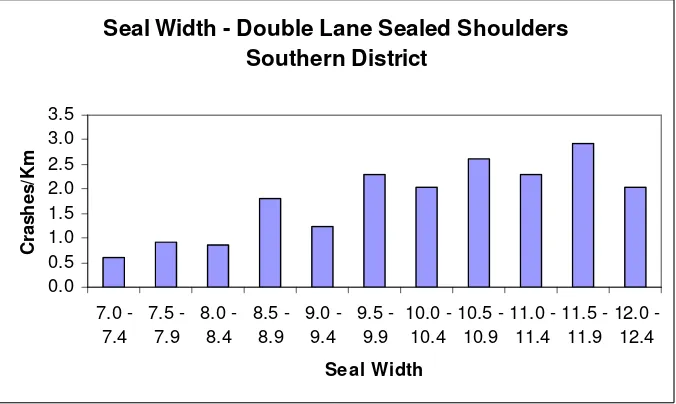
[image:60.612.139.531.354.567.2]

(61)

6.2.2 Southern District

As with the Toowoomba and Gatton districts there are only two sealed road widths that

contain enough information for an accurate analysis. Those roads were that same as

above, being double lane sealed shoulders and four lane sealed shoulders as shown in

Table 6.2 below.

The graph of double lane sealed shoulders in Figure 6.3 illustrates a good correlation.

As the width of the road increases the crashes per kilometre of road is generally

increasing. Even though the data on the length of the road for four lane sealed

shoulders is considered to be too low to present accurate statistics there is still a slight

correlation shown in Figure 6.4. This correlation is the same as in Toowoomba and

Gatton, with the crashes per kilometre increasing as the width of the road increases.

[image:61.612.164.502.420.622.2]

Seal Width - Double Lane Sealed Shoulders Southern District 0.0 0.5 1.0 1.5 2.0 2.5 3.0 3.5 7.0 -7.4 7.5 -7.9 8.0 -8.4 8.5 -8.9 9.0 -9.4 9.5 -9.9 10.0 -10.4 10.5 -10.9 11.0 -11.4 11.5 -11.9 12.0 -12.4 Seal Width C ra sh es /K m

(62)

Width # Crashes Length Crashes/Km

2.5 - 2.9 1 3.68 0.3 3.0 - 3.4 4 5 0.8 3.5 - 3.9 26 212.82 0.1 4.0 - 4.4 10 86.46 0.1

4.5 - 4.9 13 52 0.3 5.0 - 5.4 23 137.87 0.2 5.5 - 5.9 66 233.46 0.3

6.0 - 6.4 235 614.12 0.4 6.5 - 6.9 143 208.92 0.7

7.0 - 7.4 157 257.4 0.6 7.5 -7.9 121 132.23 0.9 8.0 - 8.4 181 212.61 0.9 8.5 - 8.9 162 89.806 1.8 9.0 - 9.4 383 308.892 1.2 9.5 - 9.9 186 81.19 2.3 10.0 - 10.4 204 100.03 2.0 10.5 - 10.9 127 48.88 2.6 11.0 - 11.4 130 56.67 2.3 11.5 - 11.9 99 33.86 2.9 1

Influence of physical road characteristics on road crashes