This is a repository copy of Energy metrics to evaluate the energy use and performance of water main assets.
White Rose Research Online URL for this paper: http://eprints.whiterose.ac.uk/120016/
Version: Accepted Version Article:
Hashemi, S., Filion, Y.R. and Speight, V. orcid.org/0000-0001-7780-7863 (2018) Energy metrics to evaluate the energy use and performance of water main assets. Journal of Water Resources Planning and Management, 144 (2). 04017094. ISSN 0733-9496 https://doi.org/10.1061/(ASCE)WR.1943-5452.0000857
eprints@whiterose.ac.uk https://eprints.whiterose.ac.uk/
Reuse
Unless indicated otherwise, fulltext items are protected by copyright with all rights reserved. The copyright exception in section 29 of the Copyright, Designs and Patents Act 1988 allows the making of a single copy solely for the purpose of non-commercial research or private study within the limits of fair dealing. The publisher or other rights-holder may allow further reproduction and re-use of this version - refer to the White Rose Research Online record for this item. Where records identify the publisher as the copyright holder, users can verify any specific terms of use on the publisher’s website.
Takedown
If you consider content in White Rose Research Online to be in breach of UK law, please notify us by
Energy Metrics to Evaluate the Energy Use and Performance of Water Main Assets 1
2
Saeed Hashemi1, Yves R. Filion2, Vanessa L. Speight3
3
Abstract: Managing aging infrastructure has become one of the greatest challenges for water 4
utilities, particularly when faced with selecting the most critical pipes for rehabilitation from
5
amongst the thousands of candidates. The aim of this paper is to present a set of novel yet
6
practical energy metrics that quantify energy interactions at the spatial resolution of individual
7
water mains to help utilities identify pipes for rehabilitation. The metrics are demonstrated using
8
a benchmark system and two large, complex systems. The results show that the majority of pipes
9
have a good energy performance but that an important minority of outlier pipes have a low
10
energy efficiency and high energy losses due to friction and leakage. Pumping and tank
11
operations tend to drive energy efficiency and energy losses in pipes close to water sources while
12
diurnal variation in demand drives energy performance of mains located far away from water
13
sources. The new metrics of energy lost to friction and energy lost to leakage can provide
14
information on energy performance in a pipe than is complementary to the traditional measures
15
of unit headloss and leakage flow.
16
17
Keywords: Energy efficiency, energy metrics, friction loss, leakage loss, pipe rehabilitation,
18
water distribution systems.
19
20
21
1Saeed Hashemi, Graduate Student, Queen’s University, Kingston, Ontario, Canada, K7L 3N6
(e-mail: s.hashemi@queensu.ca).
2Yves R. Filion, Associate Professor, Queen’s University, Kingston, Ontario, Canada, K7L 3N6
(e-mail: yves.filion@civil.queensu.ca).
3Vanessa Speight, Senior Research Fellow, University of Sheffield, Sheffield, UK, S1 3JD,
Introduction 22
Water distribution systems play host to a multitude of energy interactions on an hourly and
23
daily basis. Pumps and reservoirs supply mechanical energy to the system, while water demand,
24
pipe leaks, and frictional headloss provide output pathways for energy to leave the system, either
25
in the form of work or heat. As water main assets in a system age and deteriorate, they become
26
less energy efficient, with more energy leaving the system via unwanted pipe leaks and through
27
frictional headloss (Fontana et al., 2012; Kleiner and Rajani, 2001). The challenge in managing
28
a large, aging water distribution system is to prioritize interventions so that investment returns
29
the largest gain in system performance (Alvisi and Franchini, 2009 and 2006, Dandy and
30
Engelhardt, 2001).
31
Energy has long been used as a key concept to understand the performance of engineering
32
systems (Pelli and Hitz 2000; Lambert et al., 1999). Energy use as a modeling concept is
33
germane to understanding the energy performance of water main assets in distribution systems
34
because power and energy in water distribution systems depend on pressure and flow – two
35
quantities that are monitored continuously by water utilities (Dziedzic and Karney, 2015;
36
AWWA, 2009; Boulos et al., 2006). While most municipalities extensively monitor their
37
systems, few have a firm understanding of the energy efficiency of their systems. Even fewer
38
municipalities have the capability to use pressure and flow data to understand the impact of
39
infrastructure upgrades and operational changes on the energy efficiency of their systems
40
(Engelhardt et al., 2000; Roshani and Filion, 2013; Hashemi et al., 2012).
41
To date, previous research has been focused on characterizing the system-wide energy
42
dynamics in distribution systems. Colombo and Karney (2002) showed that diurnal
43
demand/pressures can affect the manner in which fissures and cracks in pipes conduct leakage.
Results demonstrated that the more distant the leakage sources are from the water sources, the
45
higher is the energy lost from leakage and friction. While, the presence of storage was shown to
46
have a negligible effect on leakage energy, the location of the tanks did influence the leakage
47
level and pumping energy (Colombo and Karney 2005). The research underscored the important
48
role of water mains, and their proximity to pumps and tanks, on the energy balance of a system.
49
Energy metrics developed thus far have focused on the system-wide energy performance of
50
systems. Pelli and Hitz (2000) developed energy indicators to relate system-wide energy
51
efficiency to pump efficiency and reservoir location, without considering leakage impacts.
52
Cabrera et al. (2010) presented a set of metrics to characterize the system-wide energy
53
performance that includes losses to friction, leakage, and overpressure. These energy metrics
54
provide a useful set of tools to help water utility managers better understand how far their
55
systems are from an ideal energy-efficient state but fall short of being able to identify individual
56
pipes that are problematic. Building upon their earlier work, Cabrera et al. (2014b) presented
57
additional metrics to assess the energy efficiency of a pressurized system and procedures to
58
prioritize interventions on a system-wide basis. Dziedzic and Karney (2014) examined the
59
energy dynamics of groups of pipes and pumps in the Toronto distribution system. While these
60
researchers also solved the energy balance to examine the frictional losses in individual pipes of
61
the Toronto system, they did not examine the efficiency, leakage, and other energy
62
characteristics of these pipes. The current paper extends this research direction by considering
63
energy transformations that take place in the individual pipes of a distribution system.
64
The aim of this paper is to present a set of novel energy metrics that quantify energy
65
interactions in a distribution system at the spatial resolution of individual water mains. These
66
pipe-level metrics can be applied to: 1) characterize the energy performance in water mains in an
unimproved state to establish a benchmark prior to any rehabilitation work; 2) plan infrastructure
68
upgrades and operational changes in areas that exhibit a low energy efficiency alongside
69
information on cost, water quality, and pipe break history, and; 3) characterize the impact of
70
infrastructure upgrades and operational improvements on the energy performance of water mains
71
in a system. In this paper, the new pipe-level metrics are applied to a large ensemble of water
72
mains across three distribution systems to examine how system operation and system
73
improvements impinge on the spatial and temporal patterns of energy performance in drinking
74
water mains.
75
Energy Use in a Pipe 76
To develop a set of energy metrics, it is instructive to consider the hydraulic grade line with
77
energy inputs and outputs in a single pipe as indicated in Figure 1. Here, the pipe conveys a flow
78
Q (m3/s) at an upstream pressure head H
s (m). The pipe delivers a pressure head Hd (m) to a
79
downstream user that imposes a demand Qd (m3/s) in the pipe. Users downstream of a pipe
80
impose a demand Qd (m3/s) that exceeds the minimum needed water use Qmin (m3/s), which
81
represents the most efficient use of water by the user given best-available water technologies
82
(Vickers 2001). There are a number of reasons for this inefficient water use including household
83
leaks, inefficiencies in appliances, theft of water (AWWA 2009), water waste through inefficient
84
industrial processes (Morales et al. 2011; Friedman et al. 2011), user perception of appropriate
85
water use (Hoekstra and Chapagain 2007), and unnecessary lawn and garden watering (Askew
86
and McGuirk 2004). For the sake of generality, the pipe can have a leak that produces a leakage
87
flow rate of Ql (m3/s). The pipe also conveys an additional flow Qds= Q-Qd-Ql (m3/s) to users
88
further downstream of the pipe. The upstream pressure head Hs (m) supplied to the pipe is
89
greater than the minimum required pressure head Hmin (m) needed to provide an acceptable
service to the downstream user. The difference between supplied head Hs (m) and pressure head
91
delivered Hd (m) is made up of local losses Hlocal (m) (e.g., valves, in-line turbines, blockages)
92
and the combined frictional head loss due to demand Qd (m3/s), leakage Ql (m3/s), and the
93
additional flow Qds (m3/s) to provide water service to downstream users. The pressure head
94
delivered to downstream users Hd (m) is made up of the minimum pressure head required, Hmin
95
(m), and surplus head, Hsurplus (m).
96
The energy components indicated in Figure 1 are defined in Table 1 and described below.
97
E
supplied=Edelivered+Eds+Eleak+Efriction+Elocal (Joules) (1)
where Esupplied = energy supplied to the upstream end of the pipe (Joules); Edelivered = energy
98
delivered to the user (in Joules) to satisfy demand Qd (m3/s) at pressure head Hd (m); Eds = energy
99
that flows out of the pipe to meet downstream user demands (Joules); Eleak = leak energy
100
(Joules); Elocal = local energy losses (Joules). The term is equal to 1.85 in the Hazen-Williams
101
friction loss model and = 2 in the Darcy-Weisbach model; K = pipe resistance and t = the
102
hydraulic time step (3,600 seconds or 1 hour) used in the 24-hour diurnal simulation.
103
Methods 104
Metrics to Evaluate Energy Performance at the Pipe Level
105
Five metrics have been developed to characterize the gross and net energy efficiencies,
106
energy needed by user, energy lost to friction, and energy lost to leakage in the pipes of a water
107
distribution network.
108
Gross and Net Efficiencies: The gross energy efficiency (GEE) in Equation 2 compares the
109
energy delivered to the users serviced by a pipe to the energy supplied to that pipe. The
110
theoretical maximum value for GEEis 100 percent, which means that all the energy supplied to
111
the pipe is delivered to its user, even though this is impossible to achieve in practice. The
theoretical minimum value for GEE is 0 percent, which means that none of the energy supplied
113
to the pipe is delivered to its users, as all the energy is lost along the pipe.
114
GEE
=
E
deliveredE
supplied 100% (2)
The net energy efficiency (NEE) in Equation 3 compares the energy delivered to users
115
serviced by a pipe to the net energy in that pipe. Here, net energy is defined as the energy
116
supplied to the pipe minus the energy supplied to users located downstream of the pipe and not
117
directly serviced by the pipe. The maximum value of NEE is 100 percent, where all the energy
118
supplied (exclusively to the pipe) is delivered to its users. The theoretical minimum value is 0
119
percent, where none of the energy supplied to the pipe is delivered to its users.
120
NEE= Edelivered E
supplied- Eds
100% (3)
Energy Needed by User: The energy needed by the users (ENU) at a node in Equation 4
121
compares the energy delivered to the users serviced by a pipe against the minimum energy
122
needed by those users. A value of ENU below 100 percent indicates that there is an insufficient
123
level of energy to meet the service expectations of the users (either in the form of flow, pressure
124
head, or both), and a value of 100 percent means that energy delivered to the users is equal to the
125
minimum energy needed to meet their service expectations. Values of ENU above 100 percent
126
denote a surplus energy over and above the level needed.
127
ENU
=
E
deliveredE
need 100% (4)
The minimum mechanical energy in the water needed to meet the minimum needs of the
128
downstream user in Equation 4 is calculated by integrating the minimum needed power by a
defined period of use t
130
E
need=
Q
minH
min
t (Joules)
(5)where = unit weight of water (approximately 9,810 N/m3 at 18oC); Qmin = minimum water
131
use needed by users (m3/s); Hmin = minimum pressure head required to deliver acceptable water
132
service to users (m); t= time step over which minimum needed power is integrated (seconds).
133
(Note that integration can be used to calculate minimum energy needed over a continuous diurnal
134
demand period.). Determining the minimum water use (Qmin) is difficult because minimum water
135
use varies between individual users within the same user type (Friedman et al. 2013). The
136
minimum pressure head (Hmin) required is usually determined by water utility standards but in
137
reality can vary across users depending on their subjective perception of the minimum pressure
138
required to perform their individualized water use activities (Mays 2002, City of Toronto 2009,
139
Region of Peel 2010, Denver Water 2012). In this paper, the minimum pressure of approximately
140
30 metres (m) commonly imposed by North American water utilities (City of Toronto, 2009;
141
Region of Peel, 2010; Denver Water, 2012) was used to calculate the minimum mechanical
142
energy.
143
Energy Lost to Friction: The energy lost to friction (ELTF) in Equation 6 compares the
144
magnitude of friction loss in the pipe (to satisfy the demand and leakage at the end of the pipe,
145
and demands downstream of the pipe) to the net energy supplied to the pipe. This indicator can
146
be used to characterize the effectiveness of pipe relining, pipe replacement, and leak repair to
147
reduce frictional losses. The metric ELTF can range between 0 and 100 percent, where a value of
148
0 percent means that there are no frictional energy losses in the pipe, and a value of 100 percent
149
means that all the net energy supplied to the pipe is lost to friction along the pipe.
ELTF
=
E
frictionE
supplied-
E
ds 100% (6)
Energy Lost to Leakage: The energy lost to leakage (ELTL) in Equation 7 compares the
151
magnitude of energy lost to leakage relative to the net energy supplied to the pipe. The leakage
152
term in the numerator includes leak energy, Eleak, and the frictional energy loss along the pipe
153
required to meet the leakage flow, Ql, at the end of the pipe Efriction(leak) (see Table 1). The ELTL
154
metric can range between 0 and 100 percent, where a value of 0 percent means that there is no
155
energy loss due to leakage in the pipe and a value of 100 percent means that all the net energy
156
supplied to the pipe is lost to leakage and friction to satisfy the leak in the pipe. The ELTL metric
157
can be used to characterize the effectiveness of leakage repair and pressure management in
158
reducing leakage energy loss.
159
ELTL= E
leak+Efriction(leak) E
supplied-Eds
100% (7)
Calculation of Energy Metrics
160
The pipe-level energy metrics presented above are evaluated by following a number of steps.
161
First, the EPANET2 (Rossman 2000) network solver is used to calculate the hydraulic head at
162
model nodes and pipe flow in model links over a diurnal period. Because the pipe flow direction
163
may change over a day, the hydraulic head at both ends of each pipe are compared at each time
164
step and the node with the higher hydraulic head is identified as the upstream node. Further, to
165
correctly recognize to which pipes a node is an upstream node and to which pipes a node is a
166
downstream node, the mechanical energy that a pipe delivers to the users at its downstream node
167
(multiple-link node) is proportional to its flow rate and is weighted by its flow rate into its
168
corresponding downstream pipes, such that
delivered
, 1 i j j m i j k k QE D H t
Q
(joules) (8)
where (Edelivered)i,j = energy delivered by pipe i to multiple-link node j (joules); Dj = demand at
170
downstream multiple-link node j located downstream of pipe i (m3/s); Hj = hydraulic head at
171
multiple-link node j located downstream of pipe i (m); Qi = flow in pipe i (m3/s); m = number of
172
k = 1, 2, 3, …, m upstream pipes connected to the multiple-link node j. For example in Figure 2a,
173
upstream pipes P-1 and P-2 with flow rates of 1.3 litres per second (L/s) and 1.6 L/s are
174
connected to downstream node J-1 (multiple-link node) with a demand of 2.1 L/s. Pipes P-3 and
175
P-4 are located downstream of node J-1. The mechanical energy ( D H t) delivered by Pipe 1
176
is weighted by the ratio of its flow to the total flow conveyed by the upstream pipes, or
177
1.3/(1.3+1.6).
178
Once the upstream and downstream nodes of each pipe have been determined, and the energy
179
delivered to each node resolved as described above, the hydraulic heads and pipe flows
180
simulated over the diurnal period are used to calculate the energy components in Table 1 to
181
evaluate the pipe-level metrics in Equations 2-7. An example is shown in Equation 9 where
182
hourly values of Edelivered and Esupplied are aggregated together throughout the day to calculate a
183
single value of GEE that is representative of the entire day
184
GEE= (Edelivered)t=1+(Edelivered)t=2+...+(Edelivered)t=24
(E
supplied)t=1+(Esupplied)t=2+...+(Esupplied)t=24 é ë ê ê ù û ú
ú100% (9)
Hydraulic Proximity Indicator
185
In the following sections of this paper, the proximity of a pipe to a water source is considered as
186
a factor that can influence the energy performance of a pipe. In anticipation of this, an indicator
Equation 10. The hydraulic proximity indicator is based on the general observation that hydraulic
189
head or pipe flow (or both) tend to decrease as one moves away from a water source to the
190
periphery of the system where pipes generally convey smaller flow to downstream users. The
191
hydraulic proximity indicator is a function of the role of the pipe (transmission or distribution)
192
and its location relative to the water source of the system or pressure zone in which it is found. It
193
is important to note that hydraulic proximity is not an indicator of the linear distance that
194
separates a pipe from a water source, but rather an indirect indicator of the proximity of a water
195
main asset to a water source.
196
4
Proximity Indicator
= Q H m s
s(
/ )
(10)in which Q is the pipe flow (m3/s) and Hs is the hydraulic head provided at the upstream node of
197
a pipe (m) calculated with the EPANET2.0 hydraulic model. (All heads are calculated according
198
to a fixed datum of 0 m.) High values of the hydraulic proximity indicator as defined in Equation
199
10 suggest that the water main is located near a water source, whereas low values suggest that
200
the main asset is located away from a water source.
201
Application of Pipe-Level Metrics to Three Distribution Systems 202
The new pipe-level metrics were applied to a large ensemble of water mains across three
203
distribution systems to examine how system operation and system improvements impinge on the
204
spatial and temporal patterns of energy performance in drinking water mains. System #1 (Figure
205
2b) is reported in Cabrera et al. (2010) and comprises 14 pipes (40 km), an elevated tank and a
206
pumping station controlled by minimum and maximum tank levels. The system has a total daily
207
demand of 79.8 ML/day with peaks at 8 am (peaking factor of 1.3) and 4 pm (peaking factor of
208
1.3) (Figure 3). Approximately 15 percent of the total demand is lost to leakage throughout the
209
day. The leakage is assigned to the nodes using emitter coefficients in EPANET2.0 (Cabrera et
al., 2010). Leakage is thus a function of time and pressure. At each time step, EPANET2 is used
211
to calculate pressure head and leakage loss to evaluate the energy lost to leakage (ELTL).The
212
average daily pressure in System #1 is approximately 35 m.
213
System #2 (Figure 4a) is a medium-sized distribution system in the US Midwest that includes
214
1,183 pipes (166 km), 4 pumping stations and 4 elevated tanks. The water distribution system is
215
comprised of three pressure zones to overcome an elevation difference of 99.7 m to serve a
216
population of 20,000 people. The system has a total daily demand of 237.9 ML/day with an 8 am
217
morning peak (peaking factor of 1.25) and a 10 pm evening peak (peaking factor of 1.67) (Figure
218
3). The daily mean pressure is 57 m and higher than in System #1. No leakage is considered in
219
this network.
220
System #3 (Figure 4b) is a large distribution network in the US Midwest that comprises
221
27,231 pipes (5,500 km), 28 pumping stations, and 27 elevated tanks that serves approximately 1
222
million customers. This system has a total daily demand of 12,765 ML/day with an 8 am
223
morning peak (peaking factor of 1.18) and a 9 pm evening peak (peaking factor of 1.40). The
224
system has an average nodal pressure of 53 m. Leakage is modelled as a constant demand
225
assigned by area to model nodes based upon the results of a detailed leakage study conducted by
226
the water utility.
227
Results 228
System #1
229
System #1 is a simple system and thus an ideal network with which to demonstrate the new
230
pipe-level metrics by way of two management scenarios (Figure 2b). The first scenario is the
231
Baseline (B) scenario where the pipes are unimproved. The second scenario is the Leakage
232
Reduction (L) scenario where pipe leakage is reduced by 50 percent by reducing emitter
coefficients in the model. In this paper, the energy metrics are dimensionless and expressed as a
234
percentage of i) energy supplied to the pipe (Esupplied), or ii) minimum energy needed at the
235
downstream node (Eneed), or iii) the net energy in the pipe (Esupplied - Eds). For the sake of
236
consistency, numerical values of the metrics that range between 0 and 30 percent are considered
237
“low”, while values that range between 30 and 70 percent are considered “moderate”, and values
238
that range between 70 and 100 percent are considered “high”.
239
Baseline Scenario (No Improvements): The baseline results in Table 2 indicate that the
240
presence of both frictional losses and leakage in the system produce low to moderate values of
241
GEE that range between 8 to 45 percent. This association is evident in the pipes closest to the
242
source and that carry higher flow rates (e.g., pipes 11, 12, 111, and 113) because these pipes
243
must convey flows destined to locations further downstream in the network. Similarly, the
244
presence of leakage in the system produces values of NEE that range between 29 to 76 percent.
245
The results in Table 2 indicate that pipes 22 and 113 have an ENU that ranges from 110 to
246
113 percent. These pipes are located between the tank (dominant source of water in this system)
247
and the highest nodal demand at junction J-22, and thus the large energy surplus reflects the
248
delivery of water to this location from the source. The pipes 31, 121, and 122 located further
249
away from the elevated tank tend to have less surplus energy, and these pipes show an energy
250
deficit and a numerical value of ENU that ranges between 91 to 97 percent; these pipes deliver
251
less energy to their users due to water losses between the sources and these demand locations.
252
The baseline values of ELTF suggest that friction losses comprise 39 to 66 percent of net
253
energy in pipes 11 and 111, both of which are in close proximity to the pumping station and
254
carry high flows. Friction comprises 1.3 to 8.0 percent of net energy in the other pipes that
255
convey smaller flows. Also, the results for leakage losses and ELTL suggest that pressure and not
leak size (as reflected in the emitter coefficient), drives the level of leakage and results in high
257
values of ELTL. For example, even though pipes 113 and 123 both have a low value of emitter
258
coefficient, their proximity to the tank in a high-pressure zone causes them to have a high
259
leakage levels and high values of ELTL that range from 18.8 to 22.2 percent.
260
The results also show that NEE in Pipe 121, located far from the tank, is driven almost
261
exclusively by the demand at the downstream node of this pipe (NEE = 55 to 61 percent from 12
262
am to 6 am; NEE = 75 to 82 percent from 6 am to 6 pm), whereas the net efficiency in Pipe 11
263
near the pump is influenced by the pumping and tank operations of the system (NEE = 10 to 20
264
percent during pumping periods of 12 am to 3 am and 1 pm to 5 pm). This finding highlights
265
how the proximity to pumps and tanks and the role of pipes in the global hydraulic performance
266
affects the net efficiency and energy lost to friction observed in individual pipes.
267
Leakage Reduction Scenario (from 15 to 8 percent of demand): The results for the leakage
268
reduction scenario in Table 2 indicate that reducing leakage flow from 15 to 8 percent produces a
269
0.2 to 11.0 percent increase in the GEE relative to baseline because it narrows the gap between
270
energy delivered and energy supplied. This relationship is especially true for the pipes located
271
further downstream (e.g., pipes 121, 122, 123, 31 and 32). Similarly, all pipes see a 3.9 to 18.8
272
percent increase in NEE relative to baseline as a result of leakage reduction. A reduction in
273
leakage also increases the ENU (or reduces the energy deficit) by 1.7 to 10.1 percent relative to
274
baseline because energy lost to leakage is decreased in the pipes. In most pipes, a reduction in
275
leakage is tantamount to reduced pipe flow and therefore less energy lost to leakage and friction.
276
For example, a reduction in leakage produces a 0.8 to 8.0 percent decrease in ELTF in pipes 112,
277
113, and 121 relative to baseline. However, in smaller pipes located further downstream in the
278
system (e.g., pipes 31, 32), the friction losses tend to increase because of an increase in pipe
flow–a result of reduction in leakage between the water source and these pipes. Lastly, a
280
reduction in leakage causes a 47.2 to 57.3 percent decrease in ELTL in all pipes.
281
System #2
282
In System #2, the energy metrics were evaluated only for those pipes (approximately 600
283
pipes or 60 percent of the total number of pipes) that have a non-zero downstream demand.
284
Because leakage was not modelled for this system, only metrics GEE, NEE, ENU, and ELTF
285
were evaluated for the baseline scenario; the impact of interventions such as leakage reduction
286
on energy dynamics was not considered. System #2 was simulated with assumed leakage levels
287
(no leakage, 15 percent, 30 percent) and the results (not shown) suggest that the presence of
288
leakage produces a similar frequency distribution of the numerical values of the four energy
289
metrics as shown in Figures 5 and 9. The absence of leakage data for System #2 does not
290
preclude the comparison of energy dynamics in System #2 with the other two systems (Systems
291
#1 through #3).
292
The histogram results in Figure 5 show that the GEE follows a bimodal distribution. Here,
293
over 60 percent of the pipes have a low value of GEE that ranges from 0 to 10 percent while
294
approximately 14 percent of the pipes have a high value of GEE that ranges from 90 to 100
295
percent. It is noted that low values of GEE in Figure 6a do not necessarily point to a poor energy
296
performance as these pipes tend to be located near the major system components and supply a
297
large number of users downstream. Pipes with a high GEE tend to be located near dead-end
298
zones where most of the energy supplied to the pipe is used to satisfy demand at the downstream
299
node of the pipe. Over 90 percent of the pipes have a NEE that ranges from 90 to 100 percent
300
(Figure 5). Figure 6b indicates that there are trunk mains and distribution mains near pumps and
301
tanks with low to high values of net efficiency (0.1 to 80 percent).
The majority of pipes (almost 80 percent) exhibit a low ELTF between 0 and 10 percent
303
(Figure 5). However a minority of pipes (almost 15 percent) had high frictional energy losses,
304
with ELTF between 90 and 100 percent. These pipes are large-diameter trunk mains that carry
305
large flows with a high average unit headloss, and are located in close proximity to a pump or
306
tank. (In this paper, average unit headloss is calculated by taking the arithmetic average of unit
307
headloss in a pipe over the 24-hour diurnal period.)
308
The energy performance of two representative pipes (Pipes 463 and 926 – see Figures 4a
309
and 6) during the 24-hour diurnal period was also examined (Figure 7). Pipe 463 is a 300 mm CI
310
water main located near pumping station P1 in System #2 and conveys flows between 15-86 L/s
311
throughout the service day. Not surprisingly, the ELTF in Pipe 463 varies in lockstep with the
312
flow in the pipe, whereby ELTF varies between 0.1 to 3 percent during low-demand periods
313
and ELTF varies between 5 to 27 percent during high-demand periods. The net energy efficiency
314
in Pipe 463 varies widely during the 24-hour diurnal period, with values of NEE between 72 and
315
86 percent during high-demand periods and values between 92 to 100 percent during
low-316
demand periods. By contrast, Pipe 926 is a 150 mm CI main located near the periphery of the
317
system (Figure 4a). This pipe conveys a near-constant flow of less than 0.10 L/s. Not
318
surprisingly, ELTF is correspondingly low (near 0 percent throughout the whole day in Figure 7)
319
and the net energy efficiency of this pipe is at a near-constant level of 100 percent. The results
320
suggest that the energy performance (in this case efficiency and friction) of a pipe is contingent
321
on the proximity of that pipe to a pump or tank.
322
The influence of the distance between a pipe and a major component on the energy performance
323
of that pipe was examined further. This was done by plotting ELTF calculated with Equation 6
324
and the max/min hourly value of energy lost to friction (ELTF-max, ELTF-min, Equation 9)
observed over the 24-hour diurnal period against the hydraulic proximity indicator (Equation 10)
326
in Figure 8 for an ensemble of 684 pipes. The results suggest that ELTF is smaller in distribution
327
mains located further away from water sources that convey low flows and incur small losses
328
(min near 0 percent). Pipes located close to water sources tend to have a value of
ELTF-329
max of 100 percent (this occurs during the peak demand period). Figure 8 shows a high variation
330
in ELTF-max in pipes located far away from water sources. This variability is likely owing to
331
differences in diameter, roughness, and service flows across the smaller water distribution mains
332
located on the periphery.
333
System #3
334
The energy metrics were evaluated for over 21,000 pipes, which represents approximately 77
335
percent of pipes in System #3. In general, the findings for System #3 are similar to those for
336
System #2 in that the frequency distribution of the numerical values of metrics follows a bimodal
337
shape (Figure 9). The bimodal nature of the results emphasizes the variability of energy
338
performance in complex systems when compared to a simpler system like System #1. The
339
majority of pipes exhibit a good energy performance (high net energy efficiency, small frictional
340
losses) and a minority of outlier pipes exhibit a poor energy performance (low efficiency, high
341
losses).
342
The histogram in Figure 9 indicates that approximately 80 percent of pipes have a value of
343
GEE that ranges between 0 and 20 percent. As noted before, low values of GEE do not
344
necessarily point to a poor energy performance; in these trunk pipes the majority of the energy
345
supplied to the pipe is transferred to users well downstream of the pipe and only a small fraction
346
of the energy is delivered to users at the end of the pipe. Figure 9 also indicates that 2 percent of
347
pipes have a value of GEE that ranges between 90 and 100 percent. In these distribution mains
near cul-de-sac areas, most of the energy is transferred to users directly at the end of the pipe.
349
Approximately 90 percent of pipes have a NEE that ranges between 9 and 100 percent (Figure 9)
350
but a minority of pipes (4 percent) have a low to moderate net energy efficiency that ranges
351
between 10 and 50 percent. A detailed analysis showed that no single factor accounted for the
352
low values of net energy efficiency in these pipes.
353
More than 95 percent of pipes have an ENUthat ranges between 100 and 120 percent (Figure
354
9) and over 90 percent of pipes have a low ELTF that ranges between 0 and 10 percent. Leakage
355
performance for this system is good with over 95 percent of pipes having a low ELTL that ranges
356
between 0 and 10 percent. Despite this generally good performance, there are a small number of
357
outlier pipes (approximately 3 percent of total) with a moderate to high ELTF that ranges
358
between 40 and 100 percent. Many of these poorly performing pipes were found to be
large-359
diameter trunk mains that convey large flows from water sources to the rest of the system. A
360
small number of pipes (2.5 percent of total) were also found to have a moderate to high ELTL
361
that ranges between 40 and 100 percent, and this is a direct result of the assigned leakage values
362
from the water utility leakage study.
363
The diurnal variation of NEE and ELTF in select pipes of System #3 were examined (results
364
not shown). As before, the results suggest that proximity to a water source and magnitude of pipe
365
flow conveyed by the pipe are both factors that have a large impact on the diurnal variation of
366
net energy efficiency and energy lost to friction. Generally, pipes located far away from water
367
sources convey little flow (with small headloss) and have values of NEE near 100 percent and
368
ELTF near 0 percent throughout the day. In larger trunk mains located closer to water sources
369
with comparatively high flow rates, NEE and ELTF track closely with diurnal variations in
370
pumped flow in these pipes, as was also observed in System #2.
The influence of the distance between a pipe and a major component on the energy
372
performance of that pipe was examined in System #3. Figure 10 plots the ELTL and the max/min
373
value of energy lost to leakage (ELTL-max and ELTL-min over a 24-hour period) for each pipe
374
(y-axis) against the hydraulic proximity indicator (x-axis). The values of the energy loss metrics
375
ELTL, ELTL-max, and ELTL-min are moderate (30 to 60 percent) near water sources (proximity
376
ranges between 3,000 and 6,000 m4/s) and moderate to high (30 to 100 percent) at the periphery
377
of the system (proximity ranges between 0 and 250 m4/s). This relationship can be explained by
378
two factors: 1) the trunk water mains close to a water source have a low level of leakage while
379
the smaller distribution mains near the periphery of the system have a higher level of leakage,
380
and 2) the values of net energy supplied to the pipe (Esupplied – Eds, denominator of ELTL) are
381
large and outweigh the energy lost due to leaks (Eleakage + Efriction(leak), numerator of ELTL)
382
because of the low level of leakage at locations near water sources. There is also a high degree of
383
variability in the values of ELTL and ELTL-max near the periphery of the system as shown in
384
Figure 10 (proximity ranges between 0 and 250 m4/s).
385
Comparison of Energy Metrics With Average Unit Headloss and Pressure Head
386
The usual practice is to use average unit headloss to identify pipes with high frictional line
387
losses and pressure head (or excess pressure head) to identify which pipes are delivering excess
388
mechanical energy to customers. Here, the energy lost to friction (ELTF) was compared to
389
average unit headloss to assess their effectiveness in identifying pipes with high frictional energy
390
losses. To do this, the five pipes with the highest values of ELTF and the five pipes with the
391
highest values of average unit headloss were selected from the ensemble of 1,183 pipes in
392
System #2 and their corresponding annual frictional energy loss was calculated. (Annual
393
frictional energy loss was calculated by multiplying the frictional energy loss in a pipe over the
24-hour diurnal period and multiplying this daily energy use by 365 days.) This was repeated for
395
System #3 (ensemble of 21,156 pipes). The results in Table 3 indicate the five pipes with the
396
highest values of ELTF and average unit headloss sorted in descending order of annual frictional
397
energy loss. Table 3 indicates that in System #2, ELTF and average unit headloss identified the
398
same four pipes (69, 159, 117, 41) with the highest annual frictional energy loss, and in System
399
#3, ELTF and average unit headloss both identified pipe 3464 as having the highest annual
400
frictional energy loss. It it noted that average unit headloss identified four pipes with higher
401
annual frictional energy loss than the ELTF. A possible reason for this is that average unit
402
headloss relates more directly to annual frictional energy loss than ELTF.
403
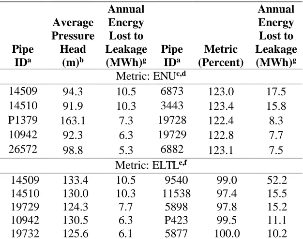
In Table 4, the energy needed by user (ENU) and energy lost to leakage (ELTL) were
404
compared to pressure head to determine their effectiveness in identifying pipes that experience
405
the highest energy losses to leakage. Similar to the above, the five pipes with the highest values
406
of ENU and the highest values of pressure head were selected from the ensemble of pipes in
407
System #3 and sorted in descending order of annual energy lost to leakage. (Annual energy lost
408
to leakage was calculated by multiplying the leak energy at the downstream node of a pipe over
409
the 24-hour diurnal period and multiplying this daily energy use by 365 days.) The results in
410
Table 4 suggest that the pipes identified with ENU and ELTL had higher values of annual energy
411
lost to leakage than those identified with pressure head. The metrics of gross energy efficiency
412
(GEE) and net energy efficiency (NEE) were not compared to average unit headloss and pressure
413
head. The interested reader can find the model data and the implementation code for the new
414
energy metrics in the supplemental data files appended to this manuscript.
415
Discussion 417
Previous research has shown that reducing leakage flow in distribution systems produces a
418
corresponding reduction in energy use (Colombo and Karney 2002, 2005). Cabrera et al. (2010)
419
found that leak-free systems required less energy per cubic metre of water delivered. Not
420
surprisingly, the observations made in System #1 of this paper corroborate these observations,
421
whereby a 50 percent reduction in leakage flow produced a near proportional decrease in energy
422
lost to leakage and improved gross and net efficiency and reduced energy lost to friction.
423
Additional observations on more realistic and more complex systems are needed to verify that
424
this near one-to-one relationship holds for most systems.
425
The analysis of Systems #2 and #3 showed that the statistical distribution of energy
426
performance of the pipes in these two large systems is bimodal where the majority of pipes have
427
a good energy performance (high efficiency, low energy losses) but that an important minority of
428
outlier pipes also have a poor energy performance (low efficiency, high energy losses to friction
429
and leakage). The research of Dziedzic and Karney (2014) showed an asymmetrical energy
430
performance across the Toronto distribution system such that water mains immediately
431
downstream of treatment works had higher energy dissipation rates than pipes located further
432
away from treatment plants. The results of the current paper corroborate this previous finding. In
433
all three systems examined, pipes near components tended to have low gross and net efficiencies
434
and high energy losses due to friction and leakage, while pipes located far away from
435
components had high gross and net efficiencies and low friction and leakage losses. Pipes near
436
components that experienced surplus pressures generally met the minimum energy needed by the
437
users (ENU > 100 percent) even if their ELTL was generally high. However, pipes in
lower-438
pressure regions further away from components generally fell short of meeting the minimum
energy needed by the users (ENU < 100 percent) and showed lower energy losses to leakage.
440
The findings of this paper showed that there is also a strong diurnal variation in energy
441
inputs and outputs at the scale of the individual pipe. For all systems examined, the diurnal
442
variation of energy efficiency and energy lost to friction in pipes close to components tended to
443
be influenced heavily by pumping periods and tank-draining periods when pipe flows and losses
444
were high in these pipes. Diurnal variation of energy efficiency and energy lost to friction in
445
pipes located far away from components tended to be more influenced by diurnal variation in
446
demand. These pipes had a low efficiency and high frictional losses during high-demand periods
447
and high efficiency and low frictional losses during low-demand periods. These finding support
448
the previous research that showed wide diurnal variations in global energy efficiencies in the
449
Toronto distribution system, where low frictional losses and high efficiencies were observed in
450
the night time when demand was low (Dziedzic and Karney 2014).
451
The results of this study also showed that the new metrics of ELTF, ENU, and ELTL may be
452
complementary indicators of energy performance in a pipe to the traditional indicators of average
453
unit headloss and pressure head. The results showed that the average unit headloss was on the
454
whole more successful than the ELTF metric in identifying pipes with the highest annual energy
455
frictional losses. This shows that average unit headloss is still an important measure because it is
456
directly tied to the pumping costs borne by a water utility. Nevertheless, the ELTF metric could
457
be used to evaluate the contribution of frictional losses relative to energy lost to leakage and
458
energy lost at the point of demand in pipes selected for rehabilitation with the average unit
459
headloss variable. Arguably, this could help water utilities understand the relative importance of
460
friction in the context of other energy losses in their system.
461
The results also suggested that the ENU and ELTL metrics are more successful than pressure
head in identifying the pipes that have the greatest energy losses to leakage. This is because ENU
463
and ELTL account for both flow and pressure head at the point of leakage that drive the
464
mechanical energy that exits the system. These results suggest that ENU and ELTL have the
465
potential to be good indicators of energy lost to leakage in distribution systems. However, the
466
results of System #1 suggest that it is the pipes that have both high pressure and high leakage
467
flow which tend to have the highest energy loss to leakage. For this reason, the results of this
468
study suggest that pressure head or leakage flow alone are not good indicators of energy lost to
469
leakage.
470
While the location of the pipe in the system has been found to have an important influence
471
on energy use, there are likely synergistic effects between the proximity to a water source and
472
other factors such as pipe diameter, pipe flow, leakage level, unit headloss that work together to
473
determine energy performance in a pipe. This paper did not examine the underlying, combined
474
effects of these key factors on the energy performance of pipes.
475
In order for the metrics of this paper to provide an accurate picture of energy performance in
476
water mains, a calibrated network model is needed with good pipe data (e.g., wall roughness and
477
diameter) and good data on the magnitude and spatial distribution of leakage. It is noted that
478
many municipalities in Canada and the US do not have good spatially-disaggregated data on
479
leakage and pipe roughness/diameter in their typically large pressure zones. Increasingly, these
480
municipalities are quantifying leakage levels and pipe flows by metering small well-defined
481
DMA (district metering area) areas that are smaller in size than traditional pressure zones. DMA
482
sectorization and flow/leak monitoring is already well-established in European countries and
483
other parts of the world and the metrics can be applied with good accuracy in these jurisdictions.
484
Previous research has shown the usefulness of energy metrics to examine the global or
system-486
wide energy performance of water distribution systems (Cabrera et al. 2010; Cabrera et al.
487
2014a, 2014b; Dziedzic and Karney 2014) and the balance between inputs and outputs of energy
488
through friction and leakage losses. The current paper offered a complementary approach in the
489
form of novel metrics that resolve energy performance at the spatial scale of the individual water
490
main. The results of the paper showed that average unit headloss is on the whole more successful
491
than ELTF in identifying pipes with high frictional energy losses, but that the new ENU and
492
ELTL metrics are more successful than pressure head in identifying pipes that experience the
493
highest energy losses to leakage. These metrics have the potential to assist water utilities in
494
understanding the energy performance of unimproved pipes alongside cost, structural and water
495
quality concerns. While outside the scope of this paper, water utilities can potentially leverage
496
this pipe-level energy analysis to perform life-cycle costing that compares the cost of pipe
497
rehabilitation against the surplus energy cost (from leakage and frictional losses) incurred in a
498
pipe when not rehabilitated (do-nothing option) to characterize the payback period of the
499
rehabilitation intervention.
500
Acknowledgements 501
The authors wish to thank the Natural Science and Engineering Research Council for its
502
financial support of this research. Dr. Speight received support from the Engineering and
503
Physical Sciences Research Council under grant EP/I029346/1. The authors also thank Mr. Brett
504
Snider from the Department of Civil Engineering, Queen’s University for his helpful comments
505
that contributed to the progress of this research.
References 507
Alvisi, S., & Franchini, M. (2006). Near-optimal rehabilitation scheduling of water
508
distribution systems based on a multi-objective genetic algorithm. Civil Engineering and
509
Environmental Systems, 23(3), 143-160.
510
Alvisi, S., & Franchini, M. (2009). Multiobjective optimization of rehabilitation and leakage
511
detection scheduling in water distribution systems. Journal of Water Resources Planning and
512
Management, 135(6), 426-439.
513
American Water Works Association (2009). M36 Water Audit and Loss Control Programs.
514
American Water Works Association, Denver, Colorado, pp. 422.
515
American Water Works Association (1991). M32 Distribution Network Analysis for Water
516
Utilities. American Water Works Association, Denver, Colorado, pp. 39.
517
Askew, L.E., and McGuirk, P.M. (2004). “Watering the suburbs: distinction, conformity and
518
the suburban garden.” Australian Geographer, 35(1), 17-37.
519
Boulos, P. F., Lansey, K. E., Karney, B. W. (2006). Comprehensive Water Distribution
520
Systems Analysis Handbook for Engineers and Planners, MWHSoft Press, Pasadena, CA, USA.
521
Cabrera, E., Pardo, M.A., Cobacho, R., and Cabrera Jr., E. (2010). “Energy audit of water
522
networks.” Journal of Water Resources Planning and Management, 136(6), 669-667.
523
Cabrera, E., Gómez, E., Cabrera Jr, E., Soriano, J., and Espert, V. (2014a). “Energy
524
Assessment of Pressurized Water Systems.” Journal of Water Resources Planning and
525
Management, 141(8), 04014095: 1-12.
526
Cabrera, E., Cobacho, R., and Soriano, J. (2014b). “Towards energy labeling of pressurized
527
water networks.” Procedia Engineering, 70, 209-217.
528
City of Toronto (2009). Design criteria for sewers and water mains. Engineering and
Construction Services, Toronto, Ontario, Canada.
530
Colombo, A.F., and Karney, B.W. (2002). “Energy cost of leaky pipes: Toward a
531
comprehensive picture.” Journal of Water Resources Planning and Management, 128(6),
441-532
450.
533
Colombo, A.F., and Karney, B.W. (2005). “Impacts of leaks on energy consumption in
534
pumped systems with storage.” Journal of Water Resources Planning and Management, 131(2),
535
146-155.
536
Dandy, G. C., & Engelhardt, M. (2001). Optimal scheduling of water pipe replacement using
537
genetic algorithms. Journal of Water Resources Planning and Management, 127(4), 214-223.
538
Denver Water (2012). Engineering Standards 14th Ed., Denver, Colorado.
539
Dziedzic, R., & Karney, B. W. (2015). Energy Metrics for Water Distribution System
540
Assessment: Case Study of the Toronto Network. Journal of Water Resources Planning and
541
Management, 141(11), 04015032.
542
Dziedzic, R. M., and Karney, B. W. (2014). “Water Distribution System Performance
543
Metrics.” Procedia Engineering, 89, 363-369.
544
Fontana, N., Giugni, M., & Portolano, D. (2011). Losses reduction and energy production in
545
water-distribution networks. Journal of Water Resources Planning and Management, 138(3),
546
237-244.
547
Friedman, K., Heaney, J., Morales, M., and Palenchar, J. (2011). “Water Demand
548
Management Optimization Methodology.” Journal of American Water Works Association,
549
103(9), 74-84.
550
Friedman, K., Heaney, J. P., Morales, M., and Palenchar, J. E. (2013). “Predicting and
551
managing residential potable irrigation using parcel-level databases.” Journal of American Water
Works Association, 105(2), 372–386.
553
Hashemi, S.S., Tabesh, M., and Ataee Kia, B. (2013). Scheduling and operating costs in
554
water distribution networks. Journal of Water Management, 166 (8), 432–442.
555
Hoekstra, A. Y., and Chapagain, A. K. (2007). “Water footprints of nations: water use by
556
people as a function of their consumption pattern.” Water Resources Management, 21(1), 35-48.
557
Kleiner, Y., & Rajani, B. (2001). Comprehensive review of structural deterioration of water
558
mains: statistical models. Urban water, 3(3), 131-150.
559
Lambert, A. O., Brown, T. G., Takizawa, M., & Weimer, D. (1999). A review of
560
performance indicators for real losses from water supply systems. Journal of Water Supply:
561
Research and Technology-Aqua, 48(6), 227-237.
562
Mayer, P. and DeOreo, W. (2010). “Improving Urban Irrigation Efficiency by Using
563
Weather-based Smart Controllers.” Journal of American Water Works Association, 102(2),
86-564
97.
565
Mays, L. (2002). Urban Water Supply Handbook. McGraw-Hill, New York, NY.
566
Morales, M., Heaney, J., Friedman, K., and Martin, J. (2011). “Estimating Commercial,
567
Industrial, and Institutional Water Use on the Basis of Heated Building Area.” Journal of
568
American Water Works Association,103(6), 84-96.
569
Pelli, T., and Hitz, H. U. (2000). “Energy indicators and savings in water supply.” Journal of
570
American Water Works Association, 92(6), 55-62.
571
Region of Peel (2010). Public Works Design, Specifications and Procedures Manual. Region
572
of Peel, Mississauga, Ontario, Canada.
573
Roshani, E., & Filion, Y. R. (2013). Event-based approach to optimize the timing of water
574
main rehabilitation with asset management strategies. Journal of Water Resources Planning and
Management, 140(6), 04014004.
576
Rossman, L.A. (2000). EPANET2: User’s Manual. US Environmental Protection Agency.
577
Cincinnati, OH.
578
Vickers, A. (2001). Handbook of Water Use and Conservation. Water Plow Press. Amherst,
579
Massachusetts.
580
Table 1. Energy inputs and outputs linked to fluid flow in a pipe.
582
Table 2. Numerical values of metrics GEE, NEE, ENU, ELTF, and ELTL for the baseline and
583
leakage reduction scenarios in System #1 (reported in Cabrera et al. (2010). GEE: Gross Energy
584
Efficiency; NEE: Net Energy Efficiency; ENU: Energy Needed by User; ELTF: Energy Lost to
585
Friction; ELTL: Energy Lost to Leakage.
586
Table 3. Pipes with the highest values of average unit headloss and energy lost to friction (ELTF)
587
in System #2 (ensemble of 1,183 pipes) and System #3 (ensemble of 21,156 pipes). (Pipes are
588
sorted by annual frictional energy loss in descending order.)
589
Table 4. Pipes with the highest values of pressure, energy needed by user (ENU), and energy lost
590
to leakage (ELTL) in System #3 (ensemble of 21,156 pipes). (Pipes are sorted by annual energy
591
lost to leakage in descending order.)
592
Table 1.
594
595
Energy Components Equations
Energy supplied Esupplied = Q Hst
Energy delivered Edelivered = Qd Hdt
Minimum energy needed to meet the end-user demand in an pipe
Eneed = Qd Hmint
Energy that flows out of pipe to meet downstream demands
Eds = Qds Hdt
Leak energy Eleak = Ql Hdt
Energy lost to friction to meet demand E
friction(demand) = K (Qd) Qdt
Energy lost to friction to meet leakage E
friction(leak) = K (Ql) Qlt
Energy lost to friction (meet d/s demand) E
friction(ds) = K (Qds) Qdst,
where Qds = Q - Qd - Ql
596
597
598
599
600
601
602
603
604
Table 2.
607
Pipe
GEE (percent)
NEE (percent)
ENU (percent)
ELTF (percent) ELTL
(percent)
B L B L B L B L B L
11 8 9 29 29 103 106 66 68 4 2
12 8 8 52 52 106 108 39 42 7 3
113 22 23 73 73 110 115 8 8 19 9
123 42 47 70 70 101 111 4 4 22 11
111 22 24 48 48 103 108 39 40 10 5
121 45 48 73 73 97 104 5 5 14 7
122 43 47 72 72 91 98 2 2 18 9
22 37 37 76 76 113 116 6 7 9 5
21 33 35 75 75 104 109 5 6 12 6
31 37 39 73 73 95 102 1 2 15 7
32 42 45 71 71 104 112 2 2 18 9
112 33 36 74 74 106 111 7 7 15 7
B = baseline scenario; L = leakage reduction scenario. 608
[image:31.612.48.549.88.335.2]Table 3. 610 611 Pipe ID Average Unit Headloss (m/km)c Annual Frictional Energy Loss (MWh)d Pipe ID ELTF (Percent)e Annual Frictional Energy Loss (MWh)d System #2
69a 470.8 2,971.6 69a 99.9*f 2,971.5
159 277.1 963.3 159 99.9* 963.3
431 131.3 644.4 117 99.9* 178.8
117 88.9 178.8 41 99.9* 150.0
41 478.2 150.0 P-97 99.9* 59.9
System #3
3464b 3.9 39,552.0 3464b 99.9*f 39,552.0 26688 2.3 28,081.6 10959 99.9* 1,313.0
9706 0.1 3,908.0 8735 99.9* 894.7
10942 0.2 1,804.4 11236 99.9* 326.0 11209 0.1 1,097.2 26528 99.9* 307.3
612
a. Pipes with the highest average unit headloss and energy lost to friction (ELTF) in the ensemble of 1,183 613
pipes in System #2 were sorted by annual frictional energy loss in descending order. 614
b. Pipes with the highest average unit headloss and energy lost to friction (ELTF) in the ensemble of 21,156 615
pipes in System #3 were sorted by annual frictional energy loss in descending order. 616
c. Average unit headloss was calculated by taking the arithmetic average of hourly values of unit headloss in a 617
pipe over the 24-hour diurnal period. 618
d. Annual frictional energy loss was calculated by multiplying the frictional energy loss in a pipe over the 24-619
hour diurnal period and multiplying this daily energy use by 365 days. 620
e. Energy lost to friction (ELTF) was calculated by taking the arithmetic average of hourly values of ELTF in a 621
pipe over the 24-hour diurnal period. 622
f. Numerical values of ELTF were truncated to the tenth of a percent in the table. 623
Table 4. 626 627 Pipe IDa Average Pressure Head (m)b Annual Energy Lost to Leakage (MWh)g Pipe IDa Metric (Percent) Annual Energy Lost to Leakage (MWh)g
Metric: ENUc,d
14509 94.3 10.5 6873 123.0 17.5 14510 91.9 10.3 3443 123.4 15.8 P1379 163.1 7.3 19728 122.4 8.3 10942 92.3 6.3 19729 122.8 7.7 26572 98.8 5.3 6882 123.1 7.5
Metric: ELTLe,f
14509 133.4 10.5 9540 99.0 52.2 14510 130.0 10.3 11538 97.4 15.5 19729 124.3 7.7 5898 97.8 15.2 10942 130.5 6.3 P423 99.5 11.1 19732 125.6 6.1 5877 100.0 10.2
a. Pipes with the highest average pressure head in the ensemble of 21,156 pipes in System #3 were sorted by 628
annual energy lost to leakage in descending order. 629
b. Average pressure head was calculated by taking the arithmetic average of hourly pressure head values in the 630
upstream and downstream nodes of a pipe over the 24-hour diurnal period. 631
c. Energy needed by user (ENU) was calculated by taking the arithmetic average of hourly ENU values in a 632
pipe over the 24-hour diurnal period. 633
d. Pipes with the highest energy needed by user (ENU) in the ensemble of 21,156 pipes in System #3 were 634
sorted by annual energy lost to leakage in descending order. 635
e. Energy lost to leakage (ELTL) was calculated by taking the arithmetic average of hourly ELTL values in a 636
pipe over the 24-hour diurnal period. 637
f. Pipes with the highest energy lost to leakage (ELTL) in the ensemble of 21,156 pipes in System #3 were 638
sorted by annual energy lost to leakage in descending order. 639
g. Annual energy lost to leakage was calculated by multiplying the leak energy (Eleak indicated in Table 1) at
640
the downstream node of a pipe over the 24-hour diurnal period and multiplying this daily energy use by 365 641
[image:33.612.150.463.98.345.2]Figure 1. Hydraulic grade line and energy inputs and outputs in a pipe.
Figure 2. a) Example calculation of energy delivered at a model node connected to upstream and
downstream pipes; b) model layout of System #1 (reported in Cabrera et al. (2010)) (L = pipe
length; D = pipe diameter; P-10 = pipe ID; J-10 = node/junction ID; Q = pipe flow; El. = node
elevation).
Figure 3. Diurnal demand pattern for Systems #1 through #3 (24-hour period).
Figure 4. a) Model layout of System #2 (medium-sized US Midwest); b) model layout of System
#3 (large-sized US Midwest).
Figure 5. Histogram that indicates the percentage of pipes with numerical values of gross energy
efficiency (GEE), net energy efficiency (NEE), energy needed by the users (ENU) and energy
lost to friction (ELTF) in System #2 (medium-sized US Midwest) for the baseline scenario.
Figure 6. a) Numerical values of gross energy efficiency (GEE) and (b) net energy efficiency
(NEE) in pipes of System #2 (medium-sized US Midwest) for the baseline scenario.
Figure 7. Hourly values of net energy efficiency (NEE) and energy lost to friction (ELTF) in Pipe
463 (near pump station P1) and Pipe 926 (located further away from pump station P1) over the
24-hour diurnal period in System #2 for the baseline scenario. (Flow in Pipes 463 and 926 are
also indicated.)
Figure 8. Energy lost to friction (ELTF) (as calculated in Eq. 6) and max/min values of energy
lost to friction observed over the 24-hour diurnal period (ELTF-max, ELTF-min) versus
proximity to a a pump or tank component in System #2 (medium-sized US Midwest) for the
baseline scenario.
Figure 9. Histogram that indicates the percentage of pipes with numerical values of gross energy
efficiency (GEE), net energy efficiency (NEE), energy needed by users (ENU ), energy lost to
friction (ELTF), and energy lost to leakage (ELTL) in System #3 (large-sized US Midwest) for
the baseline scenario.
Figure 10. Energy lost to leakage (ELTL) (as calculated in Eq. 7) and max/min values of energy
lost to leakage observed over the 24-hour diurnal period (ELTL-max, ELTL-min) versus